Recherche et adaptation des approches d’optimisation pour la conception des systèmes mécaniques

يملعلا ثحبلاو يلاعلا ميلعتلا ةرازو

Ministère de L’Enseignement Supérieur et de La Recherche Scientifique

ةعماج

سابع تاحرف

فيطس

1

Université Ferhat Abbas - Sétif 1

THÈSE

Présentée à l’Institut d’Optique et Mécanique de Précision pour l’obtention du

Diplôme de

DOCTORAT 3

ème

Cycle LMD

Domaine : Sciences et Techniques

Filière : Optique et Mécanique de Précision

Spécialité: Mécanique Appliquée

Par

FERHAT Hamza

THÈME

Recherche et adaptation des approches d’optimisation pour

la conception des systèmes mécaniques

Soutenue, le: 27/02/2021

Devant le jury composé de:

Président du Jury

Semchedine Fouzi

Prof.

UFA Sétif 1

ةيروهمجلا

ةيرئازجلا

ةيطارقميدلا

ةيبعشلا

People’s Democratic Republic of Algeria

يملعلا ثحبلاو يلاعلا ميلعتلا ةرازو

Ministry of Higher Education and Scientific Research

ةعماج

سابع تاحرف

فيطس

1

Ferhat Abbas University – Setif 1

THESIS

Submitted to the Institute of Optics and Precision Mechanics

In Partial Fulfillment of the Requirements for the Award of the Degree of

3

rd

CYCLE LMD DOCTORATE

Domain: Science and Technology

Field of study: Optics and Precision Mechanics

Specialty: Applied Mechanics

By

FERHAT Hamza

SUBJECT

Research and adaptation of optimization approaches for

design of mechanical systems

Submitted: 27/02/2021

Members of the assessment committee:

President

Semchedine Fouzi

Prof.

UFA Sétif 1

Supervisor

Djeddou Ferhat

Prof.

UFA Sétif 1

Examiner

Harrag Abdelghani

Prof.

UFA Sétif 1

Examiner

Zine Ghemari

Prof.

University of M'sila

First of all, I express my humility and utmost gratitude to ALLAH (swt) for His guidance and blessings throughout my life. Verily nonsuccess would have been achieved without His grace and mercy. It is a long journey completing this PhD dissertation. From the beginning to end, I am indebted to many individuals for their care and support given to me during this work.

I would like to express profound gratitude to my daily supervisor, Prof. Djeddou Ferhat for his valuable advices and contribution of knowledge, which made this thesis possible. He was the one who inspired and encouraged me to work on this project. His supervision, guidance and encouragement helped me tremendously.

Together with Prof. Djeddou, I would like to give special thanks to Dr. Dahane Mohammed at the National Engineering School of Metz for his invitation to visit his research group. I am very grateful for his help and time, as well as patience of revising this PhD dissertation. I hope our collaboration will go on.

I would also like to express my deepest appreciation to my co-authors: Dr. Hammoudi Abderazek, and Miss Rezki Ines. Thanks for the many fruitful discussions during the completion of this thesis and for the companionship in traveling the bumpy road towards the Ph.D. degree.

Furthermore, I would like to extend the gratitude to the members of my advisory committee, Prof. Semchedine Fouzi at the Department of Optics, Prof. Harrag Abdelghani at the Department of Precision Mechanics, and Prof. Zine Ghemari at the Department of Electrical engineering,University of M'sila.

Last but definitely not least, I would like to thank my family and friends, especially to my mother, for their ceaseless support and encouragement over the years. Thanks to all for the understanding.

Contents

Contents

List of Figures

i

List of Tables

iv

List of Symbols

vi

Introduction

1

Chapter 1. Design Optimization: An Overview

1.1 Introduction 6

1.2 Deterministic Design Optimization (DDO) 7

1.2.1 Optimization Problem Formulation 7

1.2.2 Optimization Problem Classifications 8

1.2.3 Optimization Methodologies 9

1.2.3.1 Local optimization algorithms 9

1.2.3.2 Global optimization algorithms 10

1.2.4 Multi-Objective Optimization 12

1.3 Reliability Based Design Optimization (RBDO) 14

1.3.1 RBDO Problem Formulation 14

1.3.2 RBDO Methodologies 16

1.3.2.1 Double-loop RBDO Approaches 16

1.3.2.1.1 Reliability index approach (RIA) 17

1.3.2.1.2 Performance measure approach (PMA) 17

1.3.2.2 Decoupled RBDO Approaches 19

1.3.2.3 Single-loop RBDO Approaches 20

1.3.3 RBDO with Metaheuristics 21

1.4 Comparative Study Between DDO and RBDO 23

Chapter 2. Synthesis of Cam Mechanisms: A Survey

2.1 Introduction 26

2.2 Classification and Terminology of Cam Mechanisms 26

2.2.1 Classification According to the Shape of the Cam 27

2.2.2 Classification According to the Shape of the Follower 28

2.2.3 Classification According to the Input type of Motion 29

2.2.4 Classification According to the Output type of Motion 29

2.2.5 Classification According to the Program type of Output Motion 30

2.3 Review of Cam Design Optimization 31

2.3.1 Cam Design Optimization Using Mathematical Programming Methods 31

2.3.2 Cam Design Optimization Using Metaheuristic Methods 33

2.4 Synthesis of Follower Motion Curves 34

2.4.1 Basic Motion Curves 35

2.4.2 Polynomial Motion Curves 38

2.4.3 Spline Motion Curves 41

2.5 Basic Concepts of Cam Design 43

2.5.1 Pressure Angle Analysis 43

2.5.2 Radius of Curvature Analysis 44

2.5.3 Force and Torque Analyses 45

2.5.4 Contact Stress Analysis 46

2.6 Conclusion 47

Chapter 3. Modified Adaptive Differential Evolution Algorithm

Contents

3.3.2 Improvement on the Selection Phase 52

3.3.3 Constraints Handling 53

3.3.3.1 Boundary constraints 53

3.3.3.2 Constraints functions 54

3.4 Evaluation of MADE 55

3.4.1 Three Bar Truss 56

3.4.2 Tension Spring 58

3.4.3 Welded Beam 60

3.4.4 Hydrostatic Thrust Bearing 62

3.5 Conclusion 65

Chapter 4. Optimization of Cam Mechanisms Using Metaheuristics

4.1 Introduction 66

4.2 Metaheuristics Description 66

4.2.1 Grey Wolf Optimizer (GWO) 66

4.2.2 Whale Optimization Algorithm (WOA) 67

4.2.3 Sine-Cosine Algorithm (SCA) 67

4.3 Optimum Design of Cam-Roller Follower Mechanism 67

4.3.1 Design Optimization Procedure 68

4.3.1.1 Objective functions 68

4.3.1.2 Constraints 69

4.3.1.3 Design variables 70

4.3.2 A Practical Design Example 72

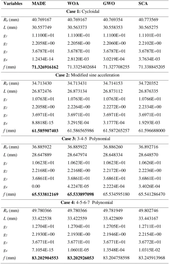
4.3.2.1 Results and discussions 74

4.4 Optimum Design of Cam Flat-Faced Follower Mechanism 80

4.4.1 Design Optimization Procedure 81

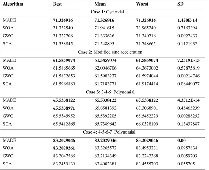
4.4.2.1 Results and discussions 84

4.5 Conclusion 90

Chapter 5. A Novel RBDO Approach

5.1 Introduction 91

5.2 Reliable Design Space (RDS) Technique 91

5.3 Nelder-Mead (NM) Simplex Search Algorithm 93

5.4 Proposed RBDO Approach: RDS-MADE-NM 94

5.5 Evaluation of RDS-MADE-NM 95

5.5.1 Cantilever Beam 96

5.5.1.1 Formulating the deterministic optimization problem 97

5.5.1.2 Results and discussions 99

5.5.2 Vehicle Side Impact 100

5.5.3 Speed Reducer 102

5.5.4 Welded Beam 105

5.5.5 Multiple Disc Clutch Brake 107

5.5.6 Cylindrical Pressure Vessel 110

5.6 Industry Case Study 113

5.6.1 Simulation Results 114

5.7 Conclusion 116

Conclusions and Future Research

118

Appendix

121

Bibliography

124

List of Figures

i

List of Figures

1 Overview of the thesis. 5

1.1 Classification of optimization methods. 9

1.2 Classification of RBDO methods. 16

1.3 Generalized flowchart of double-loop RBDO, modified from (Yu 2011). 19

1.4 Generalized flowchart of decoupled RBDO, modified from (Yu 2011). 20

1.5 Generalized flowchart of single-loop RBDO, modified from (Shan and Wang 2008).

21

1.6 Comparison results of DDO and RBDO processes. 24

2.1 Classifications of cam mechanisms. 27

2.2 Common types of cams: (a) plate cam, (b) face cam, (c) cylindrical cam, (d) wedge cam, modified from (Uicker et al. 2003).

28

2.3 Plat cams action with the common follower shapes: (a) knife-edge, (b) roller, (c) flat-face, modified from (Angeles and Lopez-Cajún 2012).

29

2.4 Program types of output motion. 30

2.5 Displacement diagrams for several basic motion laws. 36

2.6 Velocity diagrams for several basic motion laws. 36

2.7 Acceleration diagrams for several basic motion laws. 36

2.8 Jerk diagrams for several basic motion laws. 36

2.9 Displacement diagrams with different polynomial motion curves. 39

2.10 Velocity diagrams with different polynomial motion curves. 39

2.11 Acceleration diagrams with different polynomial motion curves. 39

2.12 Jerk diagrams with different polynomial motion curves. 39

2.13 Visualization of the cam pressure angle. 44

2.14 Visualization of the cam curvature radius. 45

3.1 Flowchart of the basic DE algorithm, modified from (Ho-Huu et al. 2018). 49

3.2 Flowchart of jDE technique. 52

3.3 Flowchart of feasibility rules technique. 53

3.4 Three bar truss design. 57

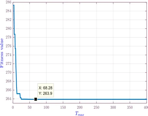
3.5 Convergence diagram of MADE for the three bar truss problem. 58

3.6 Tension spring design. 59

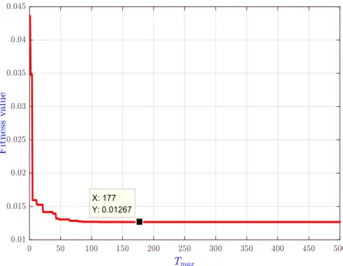
3.7 Convergence diagram of MADE for the tension spring problem. 60

3.9 Convergence diagram of MADE for the welded beam problem. 62

3.10 Hydrostatic thrust bearing design. 64

3.11 Convergence diagram of MADE for the hydrostatic bearing problem. 64

4.1 Cam mechanism with offset translating roller follower. 68

4.2 Displacement diagram of the follower motion. 74

4.3 Velocity diagram of the follower motion. 74

4.4 Acceleration diagram of the follower motion. 74

4.5 Evolution of external, inertial, spring, and total forces respect to cam rotation angle.

74

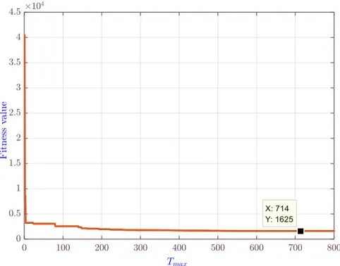
4.6 Convergence diagrams of the four algorithms for the cam design example. 76

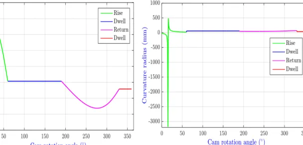
4.7 Evolution of the pressure angle. 77

4.8 Evolution of the curvature radius. 77

4.9 Evolution of the mechanical efficiency. 77

4.10 Evolution of the cam input torque. 77

4.11 Evolution of the Hertzian contact stress. 77

4.12 Optimized cam profile. 77

4.13 Non-dominated solutions obtained by NSGA-II for the cam design example. 79

4.14 Cam mechanism with translating flat-face follower. 80

4.15 Follower displacement with different motion laws. 83

4.16 Follower velocity with different motion laws. 83

4.17 Follower acceleration with different motion laws. 83

4.18 Follower jerk with different motion laws. 83

4.19 Convergence diagrams of the four algorithms for Case 1. 85

4.20 Convergence diagrams of the four algorithms for Case 2. 86

4.21 Convergence diagrams of the four algorithms for Case 3. 86

4.22 Convergence diagrams of the four algorithms for Case 4. 86

4.23 Pressure angle evolution with the modified sine curve. 89

4.24 Curvature radius evolution with the modified sine curve. 89

4.25 Optimal cam profile obtained with the modified sine curve. 89

5.1 Concept of the reliable design space. 92

5.2 Flowchart of the NM algorithm. 94

List of Figures

iii

5.6 Illustration of the RDS for the cantilever beam example. 99

5.7 Vehicle side impact design, extracted from (Youn and Choi 2004). 101

5.8 Speed reducer design. 103

5.9 Welded beam design. 106

5.10 Multiple disc clutch brake design. 109

5.11 Convergence diagrams for the multiple disc clutch brake RBDO problem. 109

5.12 Cylindrical pressure vessel design. 112

5.13 Convergence diagrams for the pressure vessel RBDO problem. 112

List of Tables

1.1 Comparison results of DDO and RBDO for the mathematical example. 24

3.1 Np size and FEs number of the MADE for each optimization problems. 56

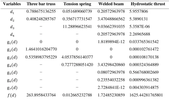
3.2 Optimal results obtained by MADE for the four engineering design problems. 56

3.3 Statistical results obtained by MADE for the four engineering design problems.

56

3.4 Comparison of MADE statistical results with literature for the three bar truss problem.

58

3.5 Comparison of MADE statistical results with literature for the tension spring problem.

60

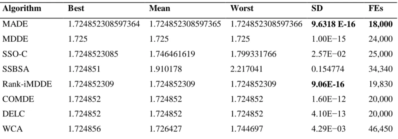
3.6 Comparison of MADE statistical results with literature for the welded beam problem.

62

3.7 Comparison of MADE statistical results with literature for the hydrostatic bearing problem.

64

4.1 Input data of the follower. 73

4.2 Input parameters of the case study example. 73

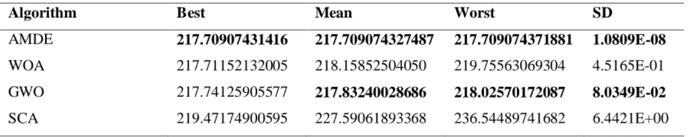
4.3 Global optimal results of the cam-roller follower mechanism. 78

4.4 Statistical results of the four algorithms for the cam design example. 78

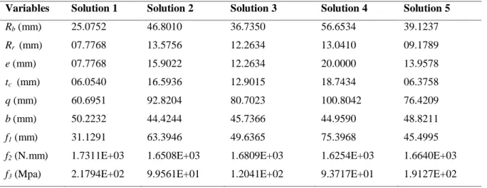
4.5 Some of the Pareto optimal solutions for the cam design example. 79

4.6 Input parameters of the case study example. 83

4.7 Global optimal results of the cam flat-face follower mechanism for the investigated cases.

87

4.8 Statistical results of the four algorithms for the investigated cases. 88

5.1 Np size and FEs number of the RDS-MADE-NM for the RBDO problems. 96

5.2 Random parameters of the cantilever beam problem. 99

5.3 Comparison of RBDO results for the cantilever beam problem. 100

5.4 Statistical results of the RDS-MADE-NM for the cantilever beam problem. 100

5.5 Random design variables and random parameters of the vehicle side impact problem.

101

5.6 Comparison of RBDO results for the vehicle side impact problem. 102

5.7 Statistical results for the vehicle side impact problem. 102

5.8 Characteristics of the speed reducer problem. 104

List of Tables

v

5.11 Random parameters of the welded beam problem. 106

5.12 Comparison of RBDO results for the welded beam problem. 106

5.13 Statistical results for the welded beam problem. 107

5.14 Random parameters of the multiple disc clutch brake problem. 109

5.15 Best results obtained by the algorithms for the multiple disc clutch brake

RBDO problem.

110

5.16 Statistical results for the multiple disc clutch brake RBDO problem. 110

5.17 Constraint value and estimated reliability of the probabilistic constraints for

the multiple disc clutch brake problem.

110

5.18 Best simulated results obtained by the algorithms for the pressure vessel

RBDO problem.

112

5.19 Statistical results for the pressure vessel RBDO problem. 112

5.20 Constraint value and estimated reliability of the probabilistic constraints for

the pressure vessel problem.

113

5.21 RBDO results of the cylindrical spur gear problem. 116

5.22 Constraint value and estimated reliability of the probabilistic constraints for

the cylindrical spur gear problem.

List of Symbols

Roman Symbols

𝐴𝑖 Control points of spline function 𝑏 Length of follower bearing 𝐵𝑖,𝑁 B-spline basis function 𝐶 Follower overhang 𝐶𝑖 Polynomial coefficients 𝐶𝑟 Crossover rate

𝑑 Vector of deterministic design variables 𝑑𝑓 Follower diameter

𝑒 Follower offset

𝐸₁ Cam modulus of elasticity 𝐸₂ Follower modulus of elasticity 𝑓 (. ) Objective function

𝐹 Cam force applied on follower 𝐹𝑒 External load

𝐹𝑓 Frictional resistance 𝐹𝑖 Inertia force

𝐹_𝑛 Normal force 𝐹_𝑠 Spring force

𝐹_𝑧 Probability density function 𝐹_1,2 Mutation factors

FEs Number of function evaluations g𝑖 Inequality constraints

𝐠_𝑖 Approximate deterministic inequality constraints 𝐺_𝑖 Performance functions

ℎ_𝑓 Lift of follower ℎ𝑖 Equality constraints

𝑘 Number of inequality constraints 𝑘𝑠 Constant elasticity of spring 𝐾 Center of cam curvature 𝐿 Length of follower face

𝑳 Lower limit of design variables 𝐿_𝑓 Follower length

List of Symbols

vii 𝑚_𝑛 Normal module

𝑀_𝑓 Follower mass

𝑛 Number of objective functions 𝑛𝑐 Number of control points 𝑁 Order of polynomial function 𝑁𝑝 Population size

𝑁𝑦 Dimension of the design variables vector 𝑁𝑧 Dimension of the random vector

𝑂 Cam rotation center

𝑝 Vector of random parameters 𝑃_𝑓 Failure probability

𝑃𝑛 Penalty function Prob(. ) Probability function

𝑞 Distance between cam center and follower bearing 𝑄 Tangency point of curvature radius

𝑟_𝑐 Control parameter of curvature radius 𝑅_𝑏 Base circle radius of the cam

𝑅_𝑒 Elastic limit of follower material 𝑅_𝑖 Structural reliability

𝑅_𝑖𝑡 _{Target reliability level} 𝑅𝑟 Roller radius

𝑠 Follower displacement 𝑠′ Follower velocity 𝑠′′ Follower acceleration 𝑡 Number of current iteration 𝑡_𝑐 Cam thickness

𝑇_𝑐𝑎𝑚 Cam input torque

𝑇_𝑚𝑎𝑥 Maximum number of iterations 𝑢_𝑧 Standard normalized vector 𝑼 Upper limit of design variables

𝑣 Tolerance allowed forequality constraintviolations

𝑣_𝑖𝑡 _{Mutated vector}

𝜐₁ Cam Poisson’s ratio 𝜐₂ Follower Poisson’s ratio 𝑤_𝑖𝑡 Trial vector

𝑤_𝑞 Weighting factors

𝑥 Vector of random design variables 𝑥𝑝1,2 Profile shift coefficients

𝑦 Vector of design variables 𝑧 Random vector

𝒛 Inverse most failure probable point 𝑧_1,2 Teeth number for pinion and wheel

Greek symbols

𝛼 Direction cosine

𝑎′ _{Distance of working center} 𝛼_𝑛 Normal pressure angle

𝛼𝑛′ Pressure angle at pitch cylinder 𝛽𝑖, Reliability index

𝛽_𝑖𝑡 Target reliability index 𝛿_𝑠 Initial deflection of spring 𝜀_𝛼 Transverse contact ratio

𝛷 Standard normal cumulative distribution function 𝜑 Cam pressure angle

𝛾𝑚𝑎𝑥1,2 Maximum specific sliding coefficients

𝜂 Mechanical efficiency

𝜇 Friction coefficient of follower / bearing 𝜇₀ Friction coefficient of cam / follower 𝜇𝑃 Mean vector of random parameters 𝜇𝑥 Mean vector of random design variables 𝜇𝑧 Mean vector of random quantities 𝜃 Cam rotation angle

𝜌 Cam curvature radius 𝜌𝑓 Radius of root curvature 𝜎 Standard deviation vector 𝜎_𝑏 Buckling critical limit

𝜎𝑐 max Maximum compressive stress

𝜎𝐹1,2 Maximum bending stresses 𝜎_{𝐻𝑚𝑎𝑥} Hertzian contact stress 𝜎_𝐻𝑝 Permissible contact stress 𝜔_𝑐 Cam angular velocity

Introduction

1

Introduction

Context and Motivation

Over the past few decades, optimization in mechanical engineering has been still a significant issue for designers and even for researchers due to the often difficulties and the high computational burden. Majority of mechanical design includes an intensive optimization task in which a number of conflicting criteria are concurrently considered, such as cost, performance, strength, and reliability. Therefore, the key challenge in the design process is to define the best compromise between contradictory design requirements. With the increasing development of computing technology during the last fifty years, several theoretical and computational contributions of optimization have been well proposed to handle the complicated design problems in the mechanics area (Gasser and Schuëller 1998; Mastinu et al. 2007; Rao and Savsani 2012).

Conventionally, optimization methods for mechanical systems design are based on the assumption of deterministic models and parameters. This is the so-called Deterministic Design Optimization (DDO) which has been effectively applied to systematically reduce the structure cost and to increase the performance. According to the search procedure, DDO approaches can be divided into two groups, mathematical programming and metaheuristic algorithms (Deb 2012). Most of the first group algorithms are inadequate to resolve the complexities inherent in the mechanical applications, as they substantially rely on the gradient information and usually seek to improve the solution in the neighborhood of a starting point. On the contrary, metaheuristic algorithms are independent of these limiting conditions and can be well suited for practical design problems. They are typically inspired by successful concepts from nature and seek to improve the solution in the whole search space.

Due to the advantages of nature-inspired metaheuristics, such simplicity, flexibility, derivative-free mechanism, and high local optima avoidance, a large number of optimization algorithms have been developed and applied to current mechanical design. Some of the most popular are Genetic Algorithm (GA), Particle Swarm Optimization (PSO), Ant Colony Optimization (ACO), and Differential Evolution (DE). In particular, the DE algorithm introduced by Storn and Price in (1995) has received increased attention from researchers because of its effectiveness and explorative ability. This algorithm can generate high-quality solutions with a good consistency, but however its performance is rather costly in terms of computational resource. Therefore, the adjustments for the DE to balance between the

computational cost and the quality of solutions have recently been one of the more interesting topics in the engineering optimization field (Jia et al. 2013; Ho-Huu et al. 2016; Mohamed

2018; Phat et al. 2020).

In practice, design optimization of mechanical systems is often highly sensitive to uncertainties derived from different sources, like structure sizes, material characteristics, manufacturing tolerances, and operating environments. Any change of these random features may significantly affect the performance of the structure to be optimized and lead to a final design with a high failure. Thus, the uncertainties are inevitable and its impact must be considered during the optimization procedure. In DDO approaches, the propagation of system uncertainties is usually handled by using the well-known safety factors. These factors, in many cases, are inaccurately adopted and cannot guarantee the desired reliability level with the most economical solution (Aoues and Chateauneuf 2010). In this sense, the Reliability-Based Design Optimization (RBDO) is emerged as an alternative and powerful tool to deal with the potential uncertainties. This methodology is capable of offering robust and cost-effective designs, and therefore has gained broad applicability in mechanics and various engineering fields (Yu 2011;Kusano et al. 2014; Ho-Huu et al. 2018; Meng et al. 2020).

Main Aim and Research Contributions

The main aim of this thesis is to contribute new optimization methods that can effectively address the complex problems of mechanical design. The present research passes through three consecutive stages. The first stage introduces an efficient deterministic optimization approach named Modified Adaptive Differential Evolution (MADE). The proposed approach is a new version of the DE algorithm with two improvements. The first improvement is carried out on the mutation and crossover phases, while the second one is executed on the selection process.

The next stage aims to apply the developed MADE for design optimization of complex mechanical systems. In this research, a particular attention has been given to cam-follower mechanism due to its flexibility and versatility in the modern industrial applications. The first problem deals with a multi-objective optimization of a cam mechanism with offset translating roller follower in which more geometric parameters and more design constraints are taken into account. The second problem concerns the size optimization of a cam mechanism with translating flat-face follower in which the influence of the follower motion law is

Introduction

3

(GWO), Whale Optimization Algorithm (WOA), and Sine-Cosine Algorithm (SCA) are employed to optimize the cam design problems.

The last stage of the thesis attempts to adapt the developed MADE toward reliability based design optimization. In this way, a novel optimization approach is presented to handle the mechanical design problems under highly uncertain manufacturing and operating conditions. The method is based on the integration of the Reliable Design Space (RDS) technique with an optimization algorithm hybridizing the MADE and the Nelder-Mead local search (NM). Consequently, the research presented in this dissertation involves three major contributions summarized as follows:

 Contribution 1:

An effective optimization method (MADE) is developed for addressing the deterministic mechanical problems with continuous design variables.

 Contribution 2:

1. The developed MADE is applied to optimize the cam mechanism design where two types of follower system are studied.

2. The optimization problem of the cam mechanism with offset roller follower translation is developed by considering additional geometric parameters and operating constraints.

3. The optimization problem of the cam mechanism with flat-face follower translation inspects the impact of follower motion by using several types of motion laws.

4. The application of three recently published optimizers (GWO, WOA, and SCA) is extended to the field of cam design optimization.

 Contribution 3:

1. A new reliability-based design optimization method (RDS-MADE-NM) is proposed to deal with the mechanical problems under the impact of uncertainties.

2. The introduced method is able to handle the mixed design variables with continuous, discrete and integer types.

3. To the best of our knowledge, the RBDO formulation for two systems is given in this study for first time and hence, new optimal solutions are presented.

Thesis Outline

Following the three contributions defined above, the thesis is structured into five chapters as illustrated in Fig. 1.

Chapter 1 gives an overview of the design optimization including the main concerns for DDO and RBDO. The basic formulations corresponding to the two processes are presented andthe related methods are reviewed.

Chapter 2 provides a literature survey on the synthesis of cam-follower mechanisms, in which the optimization of cam design and the motion curves of follower are the two interested topics. The principle classifications of these systems are also included in the chapter and the main issues of cam theory are revised.

Chapter 3 presents the variant of the DE algorithm developed in this thesis. The effectiveness of the new deterministic optimization approach is evaluated through solving four real-world engineering benchmarks, and the obtained results are compared with those available in the literature.

Chapter 4 addresses the design optimization of disc cam mechanism with translating roller and flat-face followers. For each type of follower shape, the optimization problem is formulated and an application example is presented to understand and discuss the assumptions adopted in the design process.

Chapter 5 introduces the new probabilistic optimization approach, namely RDS-MADE-NM. To confirm the search performance of this integrated approach, six mechanical design problems and a real challenging application of cylindrical spur gear are studied in the chapter.

Finally, the research findings of the thesis are summarized and recommendations for future research study are proposed.

Introduction

5

Introduction

Design Optimization Synthesis of Cam Mechanisms MADE Algorithm

A Novel RBDO Approach

Conclusion

Optimization of Cam Mechanisms Using Metaheuristics Chapter 1 Chapter 2 Chapter 3 Chapter 4 Chapter 5

Chapter 1. Design Optimization: An Overview

6

1.1 Introduction

Design optimization of engineering systems involves complex problems with several conflict considerations. The aim of engineers is the search for perfect solutions that achieve the desired objectives while satisfying the prevailing requirements. These solutions can be associated with the minimization of cost functions such as weight and material volume, or maximization of profit functions such as strength and efficiency. Nowadays, optimization takes much importance in almost every aspect of engineering design and its applications can be seen in a number of fields including, for instance, mechanics (Yildiz et al. 2019), automotive (Sun et al. 2018), civil engineering (Bekdaş et al. 2019), architecture (Ding et al.

2018), electronics (Tu et al. 2018), electricity distribution (Tan et al. 2020), and aerospace (Wu 2020; Champasak et al. 2020).

The process of solving an optimization problem is complicated by the inherently random nature of the input data. Traditional deterministic approaches for design optimization assume partial safety factors to accounts for the aleatory uncertainties. But due to the unavailability of approved rules in determining suitable values for these factors, deterministic optimization is usually imprecise and does not necessarily ensure the best balance between the economic cost and required safety (Carter 1997; Libertiny 1997). Over the last two decades, many probabilistic approaches handling uncertainties have been developed and employed to deal with engineering design (Phadke 1995; Melchers 1999; Tsompanakis et al. 2008). The well-known effective methodology is the reliability-based design optimization RBDO which quantifies closely the system uncertainties using probability theories and statistics. According to this, the design results of RBDO are more reliable and less conservative than those obtained using factors of safety concept.

In this context, the present chapter aims at giving an overview of optimization-based design considering both DDO and RBDO processes. The chapter initially deals with DDO which provides the basic knowledge of design optimization. Reliability-based design optimization is then followed in which the various methodologies are reported and the main formulations are discussed. A demonstrative example is studied in the end of this chapter to show the difference between the two processes.

1.2 Deterministic Design Optimization (DDO)

Deterministic optimization per definition refers to the process of finding the best values for design parameters of a given system without modeling the uncertainty. Conventionally, an optimization problem can be described by a vector of design variables, a n objective function and a set of constraints. The vector of design variables is the set of decision parameters that have to be determined to acquire the desired structural performance. The objective function or the fitness expresses the objectives that need to be optimized and the constraints are the conditions that must be satisfied to produce the feasible design. Additionally, there are side constraints imposed on the design variables as lower and upper bounds to define the search space. In the deterministic formulation of the design optimization problems, the design variables are assumed to be deterministic and the objective functions as well as the constraints are determined based on their nominal values (Arora 1990).

1.2.1 Optimization Problem Formulation

Typically, a design optimization problem can be defined as the search for the combination of design variable values that either minimize or maximize the objective function value while respecting certain given constraints. The standard form for a deterministic optimization problem can be mathematically given as (Deb 2012):

 

 

 

0, 1,...., ( ) 0, 1,.. min/ max : ., s.t.: i j f g d i k h find d d d d d d j m       _{ }   L U (1.1)

where 𝑑 represents the vectors of design variables, 𝑓(. ) represents the objective function, and g_𝑖(𝑖 = 1,2, … . 𝑘) and ℎ_𝑗(𝑗 = 1,2, … . 𝑚) denote, respectively, the inequality and equality constraints. The search space of design variables vector is bounded by the lower 𝑳 and upper 𝑼 limits, referred to as the side constraints. In most practical optimization problems, the fitness and the constraints are often expressed as implicit functions of the design variables and the evaluation of these functions generally involves numerical simulation techniques such as the finite element method (Rao 2019).

Chapter 1. Design Optimization: An Overview

8 1.2.2 Optimization Problem Classifications

From the standard formulation, the problem stated in Eq. 1.1 is called a single-objective, constrained, non-linear optimization problem. In fact, there are many types of design optimization problems which can be classified in several ways:

According to the number of objectives, optimization problems are classified into single-objective and multi-single-objective problems (Zhou et al. 2011). A single-objective problem has only one objective to be optimized, while a multi-objective problem involves two or more objectives to be optimized concurrently.

Based on the existence of constraints, optimization problems can be classified as constrained and unconstrained problems (Papalambros 1995). A constrained problem is stated with one or more constraints, whereas unconstrained problem is stated without constraints.

Depending on the nature of the equations involved for the objective function and the constraints, optimization problems are classified as linear and nonlinear programming problems (Arora 1990). If both the objective function and the constraints are all linear functions of the design variables, the problem is said to be a linear programming. If, however, either the objective function or the constraints are nonlinear, the problem is said to be a nonlinear programming.

According to the permissible values of design variables, optimization problems may also be classified into continuous and discrete problems (Rao 2019). Design variables of a continuous problem can take their values from within permitted intervals. In contrast, design variables of a discrete problem are restricted to take only discrete (or integer) values.

Another important criterion of classifying optimization problems is based on the type of the design variables to be considered. Accordingly, optimization problems can be distinguished into three categories:

 Sizing optimization problems: design variables of this category are associated with geometrical dimensions such as thickness of cam, module of gear, and length of beam (Haftka and Gurdal 2012; Deb 2012).

 Shape optimization problems: problems of this type include the geometry variables describing the shape of the designed parts (e.g. height of a shell) (Belegundu and Rajan 1988; Masmoudi et al. 1995).

 Topology optimization problems: problems of the last category involve design variables concerning the material distribution and the structural configuration (e.g. truss and frame structure) (Kirsch 1989; Buhl et al. 2000).

1.2.3 Optimization Methodologies

Development and application of optimization methods for engineering design is an intensive topic that has attracted increasing attention in operational research, especially with the great advance of computing technology. In the last fifty or so years, a large variety of optimization algorithms have been developed and adopted to solve various types of problems in different domains. Basically, optimization algorithms can be divided, according the optimum search mode, into two main classes: Local Optimization Algorithms, and Global Optimization Algorithms (Cavazzuti 2012; Boussaïd et al. 2013). A generalized flowchart for describing the classification of optimization methods in the literature is outlined in Fig. 1.1.

Optimization Methods

Global Optimization Algorithms

Gradient-free Algorithms

Powell’s algorithm(Powell 1964)

NM (Nelder and Mead 1965)

Local Optimization Algorithms

Gradient-based Algorithms

CGA (Fletcher and Reeves 1964)

SDA(Pallaschke and Recht 1985)

Human-based Algorithms

HS (Geem et al. 2001) TLBO (Roa et al. 2011) ISA (Gandomi 2014)

Evolutionary Algorithms

GA (Holland 1975) DE (Storn and Price 1995) BBO (Simon 2008)

Physics-based Algorithms SA (Kirkpatrick et al. 1983) GSA (Rashedi et al. 2009) RO (Kaveh and Khayatazad 2012)

Swaem-based Algorithms

PSO (Kennedy and Eberhart 1995)

ACO (Dorigo et al. 2006)

ABC (Karaboga and Basturk 2007)

Fig. 1.1 Classification of optimization methods.

1.2.3.1 Local optimization algorithms

As indicated by the name, local optimization algorithms are iterative processes that always search for the optimum in the neighborhood of a starting position. These methods typically start with the selection of an initial point and depend on specific rules for moving from one

Chapter 1. Design Optimization: An Overview

10

sequentially improved until the desired convergence is achieved (Ravindran et al. 2006; Wehrens and Buydens 2006).

Local optimization algorithms can be broadly classified into two types: gradient-based algorithms (Arora 1990;Papalambros 1995) and gradient-free or direct algorithms (Parkinson et al. 2013; Rao 2019). Gradient-based algorithms use the gradient information of the objective function and constraints to explore the search space and reach the optimum. They are mainly divided as either first-order or second order methods, depending on whether the first partial derivatives or the second partial derivatives of the functions are required. Popular examples of first-order methods include the Conjugate Gradient Algorithm (CGA) (Fletcher and Reeves 1964) and the Steepest-Descent Algorithm (SDA) (Pallaschke and Recht 1985). For the second-order methods, the well-known quasi-Newton algorithm (Rosen1966) is a good example.

Direct search algorithms, on the other hand, do not require the determination of any derivative during the search process. They are based directly on evaluating the objective function at a sequence of points and comparing their values to find the optimum. Therefore, this type of search methods is generally applicable to problems whose functions are discontinuous and its differentiation is relatively difficult (Onwubiko 2000). The most well-known examples of direct search methods are Powell’s algorithm (Powell 1964) and the simplex algorithm of Nelder and Mead (Nelder and Mead 1965). Both algorithms have a high ability to handle nonlinear, unconstrained optimization problems. Powell’s algorithm is based on the concept of conjugate directions, while the Nelder–Mead (NM) algorithm depends on a set of simple rules that reflects the worst vertex through the centroid of the simplex.

In general, local optimization algorithms are extensively used for solving optimization problems in engineering. These techniques are popular because they are efficient to attai n the optimum, using a reasonable number of function evaluations, and require little problem-specific parameters’ setting. However, these algorithms have some deficiencies which include that they often tend to obtain local optimal solutions, they are not suitable for solving discrete and multi-objective optimization problems, as they have difficulty for solving problems involving large number of constraints (Wehrens and Buydens 2006; Venter 2010).

1.2.3.2 Global optimization algorithms

In order to surmount the limitations of the methods presented in the previous section, a new class of global optimization algorithms has been introduced as adequate alternative. These

techniques, often referred to as metaheuristic algorithms, have a great capability to search in the whole design space and can provide solutions near to the global optimum. They are typically based on mechanisms inspired from nature and have the advantage of being successfully applied for complex and real-world optimization problems (Yıldız and Yıldız

2019; Abderazek et al. 2020).

Research worldwide in the metaheuristic field has produced a large number of optimization algorithms which can be classified according to several criteria in the literature (Birattari et al. 2001; Talbi 2009). By far the most common classification of metaheuristics is to take into account their original source of inspiration. In this way, they can be grouped as evolutionary algorithms, swarm-based algorithms, physics-based algorithms, and human-based algorithms. The first group contains the algorithms inspired by natural evolutionary phenomena. The two most popular techniques established here are Genetic Algorithm (GA) (Holland, 1975) and Differential Evolution (DE) (Storn and Price 1995), which simulate biological evolution processes. Other techniques that fall into this group include Evolutionary Programming (EP) (Fogel et al. 1966), Genetic Programming (GP) (Koza 1994), Evolution Strategy (ES) (Beyer and Schwefel 2002), and Biogeography-Based Optimization (BBO) (Simon 2008).

In the second group, swarm-based algorithms mimic the best features of collective behavior of animals and insects in nature. The most common techniques include Particle Swarm Optimization (PSO) (Kennedy and Eberhart 1995), which is inspired by bird flocks behavior, Ant Colony Optimization (ACO) (Dorigo et al. 2006), which is inspired by the behavior of ants in an ant colony, and Artificial Bee Colony (ABC) (Karaboga and Basturk

2007), which is inspired by the honey bee behavior. In the recent decade, many swarm intelligence techniques have been developed such as Bat-inspired Algorithm (BA) (Yang

2010), Fruit fly Optimization Algorithm (FOA) (Pan 2012), Dolphin Echolocation (Kaveh and Farhoudi 2013), Grey Wolf Optimizer (GWO) (Mirjalili et al. 2014), Whale Optimization Algorithm (WOA) (Mirjalili and Lewis 2016), and Grasshopper Optimization Algorithm (GOA) (Saremi et al. 2017).

The third group of metaheuristics includes physics-based algorithms that imitate the physical rules in the universe. Some of the well-known examples for this category are Simulated Annealing (SA) (Kirkpatrick et al. 1983), which simulates the annealing technique

Chapter 1. Design Optimization: An Overview

12

(Kaveh and Khayatazad 2012), which is based the Snell’s light refraction law.

In the last group, metaheuristic algorithms are based on the simulations of some human-related concepts. Two of the most popular human-inspired techniques are Harmony Search (HS) (Geem et al. 2001), which works on the principle of music improvisation in music players, and Teaching-Learning-Based Optimization (TLBO) (Roa et al. 2011), which works on the principle of influence of a teacher on its learners. Other popular techniques are Mine Blast Algorithm (MBA) (Sadollah et al. 2013), Social-Based Algorithm (SBA) (Ramezani and Lotfi 2013), Interior Search Algorithm (ISA) (Gandomi 2014), and recently Political Optimizer (PO) (Askari et al. 2020).

1.2.4 Multi-Objective Optimization

The discussion of deterministic optimization would not be sufficient without also mentioning the multi-objective formulation. In the wide variety of problems in engineering, the decision maker aims to optimize a number of objectives simultaneously. The different objectives are usually conflicting where the variables that optimize one objective may be far from optimal for the others. In cam design problems, for instance, minimizing the size of the cam and maximizing its strength are two objectives not compatible. Therefore, it is most necessary to compromise between the two performance criteria by selecting the appropriate values of the cam dimensions.

Formally, a multi-objective optimization problem involves multiple objectives which need to be optimized concurrently. As in single-objective optimization problem, it can contain a number of constraints that must be satisfied at any feasible solution. Since the considered objectives may be either minimized or maximized, the multi-objective optimization problem in the general form can be stated as (Deb 2001):

 

 

min/ max : ( ) . .: 1,...., 0 1,...., ( ) 0 1,..., q i j f q n g d i k h in d j m d d t d d f d s d         _{ }  L U (1.2)

where 𝑛 represents here the number of the objective functions. The problem shown above usually does not have a unique optimal solution, but rather a multitude of optimal solutions that provide a potential compromise among the objectives. These solutions are known as

Pareto-optimal solutions or non-dominated solutions (Pareto 1964, 1971).

Several techniques have been made to solve the multi-objective optimization. One of the most intuitively used is the weighted sum method, which was originally proposed by Gass and Saaty (1955). The main idea of this technique is to convert the multiple objective functions into one objective function by associating each objective with a weighting factor. In this manner, the multi-objective problem becomes a single-objective one as follows:

 

 

1 0, 1,..., ( ) 0 min/ max : ( , 1,... ) . .: , n q q q i j w g d i k h d find d f d s t d d j m d        _{ }   



L U (1.3)

The values of the weighting factors 𝑤𝑞 are selected by the decision-maker considering the relative importance of each objective. In order to find several Pareto optimal solutions, the optimization problem shown in Eq. 1.3 should be solved repeatedly through modifying the weights in the global objective function (Diwekar 2008).

Another popular alternative technique for solving multi-objective problems is the ε-constraint method, which was initially demonstrated by Haimes (1971). According to this technique, the single most significant objective function 𝑓𝑙 is optimized whereas the others are used as constraints bound by some allowed levels 𝜀_𝑞 . Thus, the new optimization problem takes the following form:

 

 

 

, 1,..., , 0, 1,... min/ max : ( ) , ( ) 0, 1,..., l q q i j f d q n find d f d l s.t q g d i k h d .: j d m d d       _   _{ }      L U (1.4)

The set of non-dominated solutions can be derived by using multiple different values for 𝜀𝑞. In this technique, the decision-maker needs to provide the range of the reference objective. In

Chapter 1. Design Optimization: An Overview

14

2009).

Apart from the conventional approaches, which turn the original multi-objective optimization into a single-objective optimization by either forming a weighted combination of the different objectives or by treating some of the objectives as constraints, there exist approaches that can solve the multi-objective problems directly, such as evolutionary algorithms (Schaffer 1984). Evolutionary algorithms for multi-objective optimization provide a set of Pareto optimal solutions by one running rather than solve a sequence of single-objective problems. Among the well-known approaches, the Non-dominated Sorting Genetic Algorithm II (NSGA-II) developed by Deb et al. (2002) is widely used due to its high resolving capacity for complex multi-objective combinatorial problems.

1.3 Reliability Based Design Optimization (RBDO)

An optimization process that accounts for feasibility in the presence of uncertainty is commonly referred to as RBDO. RBDO provides an alternative to conventional deterministic optimization and seeks for the adequate balance between cost and safety. The two main components of RBDO structure are reliability analysis and optimization (Ulucenk 2009). Reliability analysis is the inner component that focuses on handling the constraints in probabilistic term to ensure that the required level of safety is satisfied. In this framework, the random quantities involved in the constraints are quantified and their statistical characteristics are defined using apposite probability distributions. On the other side, optimization is the outer component that focuses on searching for the desired performance under the observance of the probabilistic constraints.

1.3.1 RBDO Problem Formulation

A typical RBDO is modelled as a minimization optimization problem where the lowest cost is taken as an objective and the reliability requirements are treated as constraints. In RBDO, three types of quantities are used: deterministic design variables, random design variables and random parameters. The deterministic design variables are computed based on their nominal values with negligible uncertainties, while the random design variables and random parameters are computed based on their mean values with uncertainties property being considered. Mathematically, the basic RBDO formulation can be described as follows ( Aoues and Chateauneuf 2010):

















, min : , , . .: Pr , , 0 1 , ,..., x x p t i i x x x find d d s t ob g d x p R d d d f i k              , L U L U (1.5)

where 𝑑 and 𝑥 are, respectively, the vectors of deterministic and random design variables, and 𝑝 is the vector of random parameters. The symbol (𝜇) denotes the mean of its corresponding variable, and 𝑳 and 𝑼 as in the deterministic formulation refer to the lower and upper bounds, respectively. In addition, Prob(. ) is the probability operator, and 𝑅_𝑖𝑡 is the target reliability of the ith _{constraint satisfaction specified by the designer. Here, only}

inequality constraints g_𝑖 are considered. This is because if an equality constraint involves 𝑥 or 𝑝, there may not exist a solution for any arbitrary desired reliability against failure (Deb et al. 2009).

For convenience of discussion and to avoid confusion in this thesis, we assume that 𝑦 = {𝑑, 𝜇_𝑥} is the vector of design variables, and 𝑧 = {𝑥, 𝑝} is the random vector. 𝑁𝑦 and 𝑁𝑧 are the dimensions of the vectors 𝑦 and 𝑧, respectively.

-The concern in evaluating the probabilistic constraint is to employ the following integral:

 





_{ , 0}

 

Prob , 0 i i _{g d z} z g d z F z dz   



(1.6) where 𝐹𝑧 represents the joint probability density function of the vector 𝑧. Theoretically, the exact computation of this integral is very difficult owing to the absence of analytical solvers. Simplest techniques based on stochastic simulations such as Monte Carlo Simulation (MCS) (Mooney 1997) and Subset Simulation (SS) (Au and Beck 2001) are usually used and considered as reference methods. However, the major drawback of these methods lies in the high number of function evaluations. To deal efficiently with the integral in Eq. 1.6, moment techniques such as the first and second-order reliability methods (FORM/SORM) (Hasofer and Lind 1974) (Breitung 1984) can be employed. The idea is to map the constraint function g𝑖 from the original design space (𝑍 space) to the standard normal space (𝑈 space), and then establish the linear (or quadratic) approximation of the function at the point of maximum likelihood, known as the most probable failure point (MPFP), for estimating the reliability (Madsen et al. 2006). The passage from the 𝑍 space to the 𝑈 space can be achieved based the

Chapter 1. Design Optimization: An Overview 16 1 1 ) ( ), 1, 2,..., . ( ( )), ( )) ( ( zj j j zj j j j j zj Φ u C j Nz DF z u Φ CDF z z CDF Φ u     (1.7) where 𝛷 and 𝛷−1 _{are respectively the standard normal cumulative distribution function and} its inverse function. 𝐶𝐷𝐹𝑗 and 𝐶𝐷𝐹𝑗−1are the cumulative distribution function and its inverse function of 𝑧𝑗, respectively. 𝑢𝑧 denotes the vector 𝑧 in the standard normal space.

1.3.2 RBDO Methodologies

The main challenge in the resolution of RBDO problem (Eq 1.5) is associated with the evaluation of the probabilistic constraints, as they require high numerical efforts. Many researches have been developed in the past few decades, aiming to overcome this difficult task, which are still the key obstacle for practical engineering applications. According to the strategies used to deal with the probabilistic constraint during the optimization process, RBDO methodologies can be classified basically into three categories: namely double-loop approaches, decoupled approaches, and single-loop approaches, as shown in Fig. 1.2.

RBDO Methods

Double-loop Approaches

RIA (Nikolaidis and Burdisso 1988)

PMA (Tu and Choi 1999)

Single-loop Approaches

SLSV (Chen et al. 1997) SLA (Liang et al. 2008) RDS (Shan and Wang 2008) SLDM (Li et al. 2013)

Decoupled Approaches

SORA (Du and Chen2004) SAP (Cheng et al. 2006) ADA (Chen et al. 2013) ISV (Huang et al. 2016)

Fig. 1.2 Classification of RBDO methods.

1.3.2.1 Double-loop RBDO Approaches

The basic RBDO methodology employs a double-loop procedure in which the probabilistic constraints evaluation is included in the main optimization loop (Fig. 1.3). This formulation leads to a nested optimization problem where the inner loop concerns the reliability analysis and the outer loop concerns the cost optimization (Wu 1994; Yu et al. 1998; Youn et al.

2003). The two popular techniques encountered in this category are Reliability Index Approach (RIA) and Performance Measure Approach (PMA). RIA technique has been proposed by Nikolaidis and Burdisso (1988) and its principle is to search for the MPFP on the limit surface using the reliability index concept. This technique is simple to formulate, but it

requires considerable computational efforts and converges slowly owing to difficulties to compute the constraints reliability (Enevoldsen and Sørensen 1994). To overcome these drawbacks, Tu and Choi (1999) have developed the performance measure approach in which the probability evaluation is converted into a performance measure by solving an inverse reliability problem. The obtained solution of this inverse problem represents the minimum performance point on the target reliability surface, known as the minimum performance target point (MPTP).

1.3.2.1.1 Reliability index approach (RIA)

The classical RBDO formulation based on the reliability index approach is expressed as:

 





( , min : , . .: ) , 1,..., z t i i f d z find y d s t y i k y y       L U (1.8)

where 𝛽_𝑖 and 𝛽_𝑖𝑡 denote respectively the structural and the target reliability indexes of the ith

probabilistic constraint. Through transforming the random vector 𝑧 to the independent standard normalized vector 𝑢_𝑧 (using Eq 1.7), the reliability index 𝛽_𝑖 is calculated by solving the following minimization problem:

 





2 1 min : . : , 0 Nz i j z j i z z find u u s t G d u    



(1.9)

The optimal solution of this problem is the MPFP in the 𝑈 space, and can be obtained using some well-established algorithms such as the HL-RF iterations (Hasofer and Lind 1974; Rackwitz and Fiessler 1978) or the improved HL-RF iterations (iHL-RF) (Madsen et al.

2006). According to FORM approximation (Haldar and Mahadevan2000), the reliability 𝑅_𝑖 is given by: 𝑅_𝑖 = 𝛷( 𝛽_𝑖 ).

1.3.2.1.2 Performance measure approach (PMA)

The basic idea of the performance measure approach is that optimizing a complex objective function under simple constraints is much easier than optimizing a simple objective function

Chapter 1. Design Optimization: An Overview 18

 





( , min : , . .: ) 0, 1,..., z i f d z find y d s t y y i G k y      L U (1.10)

where 𝐺𝑖 is the ith performance function evaluated by the inverse reliability analysis. Unlike the RIA-based RBDO, which searches for the minimum distance point from the mean values of the vector 𝑧 to the failure surface subject to null limit state functions, the PMA tries to find the failure point corresponding to the lowest performance that satisfies the target reliability index:

 





2 1 min : , . .: z i z zj Nz t i j find u G d u s t u   



(1.11)

The optimal solution of the previous problem is the MPTP in the 𝑈 space, and can be obtained using many specific algorithms, such as the Advanced Mean Value (AMV), the Conjugate Mean Value (CMV) and the Hybrid Mean Value (HMV) (Youn et al. 2005). These approaches do not require a line search procedure because the search direction is simply determined by exploring the spherical equality constraint in Eq. 1.11. The accuracy and stability of PMA is demonstrated when compared with RIA in the study of Lee et al. (2002).

Probabilistic constraints Constraint 1 Constraint 2 Constraint k Convergence ? Optimal Design Yes Start Point Optimization Loop No Reliability Analysis Probabilistic Constraints Reliability Analysis Reliability Analysis

Fig. 1.3 Generalized flowchart of double-loop RBDO, modified from (Yu 2011).

1.3.2.2 Decoupled RBDO Approaches

The RBDO using RIA or PMA requires an expensive computation due to the repeated evaluation and analysis in both reliability and optimization loops. To overcome this difficulty, several researchers have focused on developing more computationally efficient RBDO methodologies, based on either decoupled or single loop procedures. Decoupled techniques have been introduced to separate reliability analysis from optimization process and thus, the evaluation of probabilistic constraints is not carried out within the main optimization loop (see Fig. 1.4). The most common approach in this category is the Sequential Optimization and Reliability Assessment (SORA), developed by Du and Chen (2004). The SORA approach consists in transforming the double loop in RBDO into a sequence of deterministic optimization and reliability analyses where the reliability information obtained from the previous cycle are used to shift the boundaries of the violated deterministic constraints to the feasible region. In this way, the design solution is improved from cycle to cycle until convergence.

Chapter 1. Design Optimization: An Overview

20

There are many other approaches that use the decoupling strategy. For example, Royset et al. (2001) have decoupled the reliability analysis from optimization by using the concept of Semi-Infinite Programming (SIP) (Kirjner-Neto et al. 1998) where the failure probability constraints have been replaced by a parameterized first order approximation. The Sequential Approximate Programming (SAP) approach has been developed by Cheng et al. (2006) where the RBDO has been formulated as a sequence of deterministic sub-programming problems and the probabilistic constraints have been approximated by the first order Taylor series expansion. Authors in (Li et al. 2010) have proposed the Penalty-Based Approach (PBA) using the penalty concept in order to link the reliability requirement to the deterministic optimization. Chen et al. (2013) have introduced the Adaptive Decoupling Approach (ADA) based on the concept of SORA. Furthermore, Huang et al. (2016) have developed another efficient decoupling approach, known as Incremental Shifting Vector (ISV), based on the shifting vector technique.

Convergence ?

Optimal Design Yes No

Relability Analysis Supplying Sensitivity Information

Start Point

Deterministic Design Optimization

P

Min Objective function Deterministic constraints Side constraints S.t

Fig. 1.4 Generalized flowchart of decoupled RBDO, modified from (Yu 2011).

1.3.2.3 Single-loop RBDO Approaches

In addition to double-loop and decoupled approaches, the single-loop techniques have been introduced to convert the nested optimization loops into one loop by eliminating the inner

reliability loops (Fig. 1.5). This type mainly contains iterative single-loop approaches and complete single-loop approaches. The first subgroup of approaches employs an iterative procedure based on the Karush-Kuhn-Tucker (KKT) conditions to remove the reliability analyses, such as the Single Loop Single Vector (SLSV) (Chen et al. 1997) and the Single Loop Approach (SLA) (Liang et al. 2007; Liang et al. 2008). Whereas the second subgroup employs a direct procedure through substituting the probabilistic constraints with approximate deterministic ones in one step. Two approaches have been developed in this context, the Reliable Design Space (RDS) method (Shan and Wang 2008) and the Single-Loop Deterministic Method (SLDM) (Li et al. 2013). Both approaches have the same strategy that uses the partial derivatives at the current design point as an approximation of the derivatives at its corresponding MPFP. However, RDS method is derived from RIA while SLDM reaches the formulation based on PMA.

Conversion of Probabilistic constraints RBDO Formulation DDO Formulation Optimal Design Opimization loop

Fig. 1.5 Generalized flowchart of single-loop RBDO, modified from (Shan and Wang 2008).

1.3.3 RBDO with Metaheuristics

In the last few decades, the use of metaheuristic algorithms to solve RBDO problems has rapidly increased, mainly due to the development of sophisticated computing technologies and the extensive applications of the Finite Element Analysis (FEA). Following the double-loop approach, António (2001) has applied the genetic algorithm GA for RBDO of composite