Any correspondence concerning this service should be sent to the repository administrator:
[email protected]
This is an author-deposited version published in:
http://oatao.univ-toulouse.fr/
Eprints ID: 6555
To cite this version
:
Xu, Jiucheng and Archimède, Bernard and Letouzey, Agnès Shared resources
scheduling using a multi-agent model: the DSCEP framework.
In: 9th
International Conference of Modeling, Optimization and Simulation -
MOSIM’12, 06-08 June 2012, Bordeaux, France.
O
pen
A
rchive
T
oulouse
A
rchive
O
uverte (
OATAO
)
OATAO is an open access repository that collects the work of Toulouse researchers and
makes it freely available over the web where possible.
SHARED RESOURCES SCHEDULING USING A MULTI-AGENT MODEL:
THE DSCEP FRAMEWORK
J. XU, B. ARCHIMÈDE, A. LETOUZEY
University of Toulouse, INPT-ENIT 47, Avenue d’Azereix, BP1629 F-65016 Tarbes Cedex - France
[email protected], [email protected], [email protected]
ABSTRACT: Recently, agent systems have been successfully applied to the scheduling problem. A new
multi-agent framework, called DSCEP (distributed, supervisor, customers, environment, producers), is suggested in this paper. This framework is developed base on the subsistent SCEP models, especial for shared resources scheduling activities. It introduces a dialogue between three kinds of evolved SCEP models leading to a high level of co-operation. It provides a more efficient control of the consequences generated by the local decisions than usual systems for each SCEP model. It also provides different algorithms in order to handle the disturbances occurring at different ranks in manufacturing process. As a consequence, the DSCEP framework can be adapted for various scheduling/planning problems. This model is applied to the shared resources scheduling problem of complex systems, and provide a natural cohabitation between infinite capacity scheduling processes, performed by the multi-site manufacturing orders, and finite capacity scheduling processes, performed by local or remote machines.
KEYWORDS: shared resources, distributed scheduling, DSCEP, multi-agent systems, disturbances.
1. INTRODUCTION
In recent years, shared resources problem is studied as a hot spot issue because the resources in a single organiza-tion seem to be limited to fit for the rapidly changing market environment. The initial definition of shared re-source is mentioned in computer science area, it is either a device or piece of information on an accessible com-puter from another comcom-puter, transparently as if it were a resource in the local one (Galvin, 1994). Extending to manufacturing field, shared resources can be any kind of useful resources during the manufacturing process. The-se resources belong to enterpriThe-ses (organizations) with independent accounting and different geographical posi-tions, but can be required by each other.
The purpose of scheduling is to minimize the production time and costs, by telling a production facility when to make, by which staff, and on which equipment (Blazewicz et al., 2001). For shared resources schedul-ing, each organization independently construct a local schedule to satisfy its own purposes. These local sched-ules will lead to conflicts and disturbances for the global scheduling of shared resources. The complexity of the shared resources problem is also caused by prisoner's dilemma (Le and Boyd, 2007). To avoid this, we can build a virtual enterprise (Molina and Sanchez, 1998) to encourage organizations to share resources with partners. In this communication, we will introduce a new multi-agent framework DSCEP which focus on the shared re-sources problems in complex systems, like manufactur-ing factories, hospitals, and transport systems etc.
This paper is organized as following: section 2 reviews the different multi-agent technologies and discusses their limitation. Section 3 gives a brief introduction of the multi-agent model SCEP. Following, we provide a DSCEP framework in order to better identify shared re-sources solution with disturbance in section 4. Section 5 describes the scheduling process using the DSCEP framework particularly focuses on a hospital system case study. A brief conclusion and perspectives are stated in section 6.
2. SCHEDULING TECHNIQUES WITH MULTI-AGENT SYSTEMS
2.1. Multi-agent approach for job shop scheduling
Multi-agent systems (MAS) are the subfield of Distrib-uted Artificial Intelligence (DAI) which has experienced rapid growth since the available flexibility and intelli-gence could solve distributed problems (Balaji and Srinicasan, 2010). The multi-agent approaches can cope with conflict situations with negotiation technologies, in which the compromises can moderate the satisfaction and frustrations of the agents.
For the dynamic scheduling and shop floor job assign-ment problem, a real-world manufacturing system in a multi-agent system has been represented, and further-more improves the global performance by introducing Ant Colony Intelligence (ACI) into agent coordination and negotiation. (Xiang and Lee, 2008). A distributed
multi-agent scheduling system (MASS) based on co-operative approach is proposed to solve static and dy-namic job shop scheduling problems (JSSP) (Kouider and Bouzouia, 2012). This system is composed of two kinds of agents, Supervisor agents and Resource agents. The Supervisor agent decomposes JSSP into interrelated sub-problems and the Resource agents co-operate, through a distributed approach of local idle time minimi-zation.
Two Multi-Agent approaches based on the Tabu Search (TS) meta-heuristic have proposed by (Ennigrou and Ghedira, 2008). Depending on the location of the opti-mization core in the system, they have distinguished between the global optimization approach where the TS has a global view on the system and the local optimiza-tion approach (FJS MATSLO) where the optimizaoptimiza-tion is distributed among a collection of agents, each of them has its own local view. A multi-agents approach to solve job shop scheduling problem using meta-heuristics is presented by (Passos et al., 2010). Meta-heuristics ap-proaches when solving scheduling problems have proven to be very effective and useful in practical situations. TS and Genetic Algorithms (GA) have been used to solve optimization problems with success. This approach combining these algorithms brings new perspective to solve this kind of problem. Another multi-agent architec-ture of an integrated and dynamic system is also devel-oped for process planning and scheduling of multiple jobs. A negotiation protocol is discussed to generate the process plans and the schedules of the manufacturing resources and the individual jobs, dynamically and in-crementally, based on the alternative manufacturing pro-cesses (Nejad et al., 2011).
2.2. Synthesis
From the approaches mentioned in previous section, agent-based approaches have several potential ad-vantages for distributed manufacturing scheduling (Shen et al., 2006).
They use parallel computation through a large num-ber of processors, which may provide scheduling systems with high efficiency and robustness.
They can facilitate the integration of manufacturing process planning and scheduling.
They make it possible for individual resources to trade off local performance to improve global per-formance, leading to cooperative scheduling. Resource agents may be connected directly to
phys-ical devices they represented for so as to realize re-al-time dynamic rescheduling.
Schedules are achieved by using mechanisms simi-lar to those being used in manufacturing supply chains.
These existing multi-agent systems have been success-fully applied to the job shop scheduling problem, but they are not taking into account shared resources
sched-uling in complex system. So, we will describe a multi-agent model named SCEP in next section, which have capabilities to handle shared resources scheduling prob-lem in certain conditions.
3. SCEP MULTI-AGENT MODEL 3.1. Architecture of SCEP model
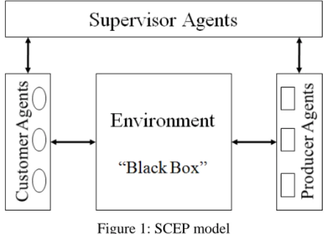
The SCEP multi-agent model is briefly a distributed model developed for all types of planning activities, which introduces an indirect cooperation between two communities of agents (customer agents called C and producer agents called P), leading to a high level of co-operation. Each customer agent manages one order from the customers; each producer agent manages one re-source (machine, raw material or human) of the organi-zation. The cooperation between customer agents and producer agents is performed synchronically through the background environment agent E. The supervisor agent S controls all the activities (Archimede and Coudert, 2001). We can see the architecture of SCEP model in figure 1. The detail working procedures and dynamic of the model will be introduced in next section.
Figure 1: SCEP model
3.2. Description of SCEP model
Each object in the environment is associated with one operation to be achieved in one customer order. The set of objects are related to the routing followed by the intervention domain of concerned agents. In perfect correlation with the model definition, each operation only concerns one customer agent. But some objects can belong to the intervention domains of several producer agents, because multi machines may achieve the same activity. The format position of object O is [(S, F), N], where (S, F) represents a continuous temporal interval between starting date S and final date F, N represents the identity of resource which executing object O. Each object has four kinds of position, wished position (WP), effective position (EP), potential position (PP), and confirmed position (CP). The WP is the position requested by the customer. The EP results from the scheduling of all the tasks associated with the propositions collected from the environment. The PP
results from the scheduling of one task associated with a proposition collected from the environment. The CP is the final position after all the scheduling process.
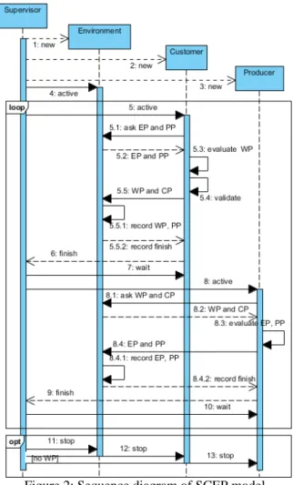
The supervisor agent provides functions of creating the agent society, generating the inside objects and initializing the environment. Then, the supervisor agent triggers the cycle of cooperation process by activating the customer agents and telling the producer agents to wait. The customer agents firstly ask for EP and PP of the associated objects from the environment. The environment sends the results back, of course the result is null in the first cycle. The customer agents schedule the operations which have not been validated, and influence the associated objects by alterative WP. If the wished position of one object is the same as the effective position and potential position, customer agents will make the confirmation. At last, the customer agents send CP and WP of the associated objects to the environment. Each customer agent performs its actions simultaneously but remains independently from others. It will inform the supervisor agent once its actions are finished.
Figure 2: Sequence diagram of SCEP model Once the end of the action from the last customer agent has been recorded by the environment, the supervisor agent activates the producer agents and sends the wait signal to the customer agents. The producer agents firstly
ask for the CP and WP of the objects belonging to its intervention domain from the environment. The envi-ronment sends the results back; the producer agents rec-ord the CP and schedule the tasks which are not definite-ly positioned. They influence these objects by alterative EP and PP to the environment. Each producer agent per-forms its actions independently and inper-forms the supervi-sor agent as soon as its activities finished. When the end of the action from the last producer agent is recorded, the supervisor agent finishes the first cycle of the coopera-tion and starts the next cycle immediately. In each cycle (except the first one), at least one object should be con-firmed in order to avoid the deadlock problem. The fig-ure 2 shows the detail working procedfig-ure of SCEP mod-el.
The alternation cycle between the activation of customer agents and producer agents is repeated until the CP of all the environmental objects is effective. When entire ob-jects are confirmed, there are no WP from customer agents anymore. The alternative (opt) area will be exe-cuted and the supervisor agent will terminate the envi-ronment, customer and producer agents. The whole scheduling process is finished.
3.3. Dynamic of SCEP model
In this section, the formalism used to show the conver-gence of this model is presented. The environment E is composed of a set of objects O that evolve according to the influence that they receive from the customer and producer agents.
The SCEP model has been used for the production scheduling and maintenance scheduling. In SCEP model, the customer agents share resources managed by various producer agents. However, it only works with the re-sources/orders managed by producer/customer agents inside the same site. In order to share resources located in remote sites, an evolved SCEP model has been devel-oped (Xu et al., 2011). This model showed its adaptation to the distributed management of multi-site orders. Alt-hough the evolved SCEP offers to solve the distributed scheduling problem, it only enables resources sharing between orders from the same site. As extension, we propose a DSCEP framework to achieve multi-site and shared resources scheduling between different (both economic and geographical) organizations.
4. DSCEP FRAMEWORK FOR SHARED RESOURCES SHCEDULING
4.1. Evolution and classification for SCEP model
In order to fit the requirements of shared resources scheduling, we extend the SCEP model with virtual cus-tomer agent (VC) and virtual producer agent (VP). Each VC manages entire orders from another SCEP model and basic customer agents manage entire orders from the local one. Each VP manages resources from another
SCEP model and each basic producer agent manages entire resources of the local one. The example of evolved SCEP model is shown in figure 3.
Figure 3: Evolved SCEP model
We classify the evolved SCEP model into three catego-ries based on the following rules. Root SCEP models are evolved SCEP models, which do not manage shared re-sources but require shared rere-sources from others. On the opposite side, leaf SCEP models are evolved SCEP models, which provide shared resources but do not re-quire from others. The third category is internal SCEP models; these internal SCEP models not only manage shared resources but also require shared resources from others. As we introduce in previous section, the ability of the VP and VC is fixed. So the root SCEP only has sev-eral VP, the leaf SCEP only has sevsev-eral VC, and the in-ternal SCEP must have both of them. The VC and VP should be one-one correspondence in the whole frame-work.
4.2. Architecture of DSCEP framework
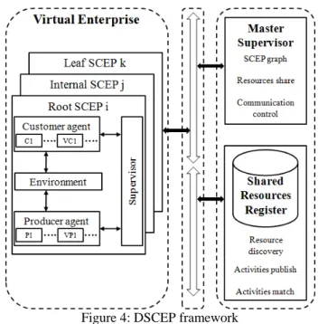
We propose the DSCEP framework to synchronize and control the use of evolved SCEP models in order to elaborate or adapt a schedule involving shared resources. The whole framework is composed by three kinds of elements: virtual enterprise, shared resources register, and master supervisor. The communications between these elements are made through the communication bus in the framework. We can see the architecture of DSCEP framework in figure 4.
The virtual enterprise is an imaginative enterprise based on the ability to create temporary co-operations and to realize the value of a short business opportunity that the partners cannot (or can, but only to lesser extent) capture on their own. Each member of this virtual enterprise is managed by an evolved SCEP model.
The shared resources register is a database which records all the public activities provided by shared resources. It can use an ontology mechanism to match the activities requirements from evolved SCEP models with the pub-lished activities recorded in the register.
Figure 4: DSCEP framework
The master supervisor is a controller which records the existing of entire SCEP models and the connection in-formation of them. It divides SCEP models into three categories based on the ordered graph technology (Dechter, 2003). It also manages all the communication activities between SCEP models and shared resources register.
4.3. Dynamic of DSCEP framework
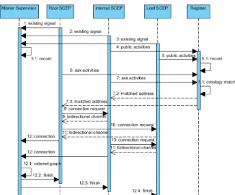
Each member of the virtual enterprise creates an evolved SCEP model based on the rules we introduce in the pre-vious section. After their creation, all SCEP models send an existing signal to the master supervisor. Leaf and in-ternal SCEP models publish the public activities provid-ed by sharprovid-ed resources to the sharprovid-ed resources register. Root and internal SCEP models call register to get the address of the corresponding leaf and internal SCEP models. In order to identify these addresses, the register achieves matching between required and recorded activi-ties by an ontology mechanism, and sends the result back. Then the root and internal SCEP models send the connection requests to the corresponding leaf and inter-nal SCEP models, which have shared resources. A peer to peer bidirectional communication channel will be es-tablished between one virtual producer agent and one virtual customer agent for each couple (A and B) where A is an root/internal SCEP requiring public activities and B is an leaf/internal SCEP providing these activities. After the channel is build, root/internal SCEP models send connection information to the master supervisor. Then, the first step of DSCEP scheduling process is fin-ished. The figure 5 shows the detail working procedure.
Figure 5: Sequence diagram of DSCEP scheduling step 1 The master supervisor builds and maintains an ordered graph for entire evolved SCEP models, in order to control and synchronize the global scheduling process. In this graph each node is associated with an evolved SCEP model; each directed segment is associated with a unidirectional invoking of shared resource. All nodes on rank 0 should be root SCEP (RS) models and all nodes on the last rank n should be leaf SCEP (LS) models. The nodes on rank m (0<m<n) are internal SCEP (IS) models. The figure 6 is an example of ordered graph for DSCEP framework.
Figure 6: Ordered graph for DSCEP framework The second step of DSCEP scheduling process is shown in figure 7. First of all, we give the definition of sub-tree, the sub-tree of node x (in rank i) is a set of nodes in rank j (j>i) which contains all the shared resources required by x. For example, {IS1, IS2, IS3, LSn} is the sub-tree of
node RS2. The orders defined in node x can exploit all
the shared resources located in the nodes which belong to the sub-tree of node x. No matter in which rank, the scheduling process of an evolved SCEP model x will be achieved in finite number of cycles, as we described in the section 3.
Figure 7: Sequence diagram of DSCEP scheduling step 2 In each cycle, a complete scheduling will be achieved for all the evolved SCEP models in the sub-tree of x. These schedules may be partially cancelled at new cycle. The scheduling process will be finished when all the orders defined in the parent node x are scheduled. The global scheduling is achieved periodically. In that case, the scheduling process will be launched for all nodes in rank 0 at the same time. When node y detects a perturbation (receives new orders), a partial scheduling will be launched only for y and nodes belonging to the sub-tree of y.
4.4. Mathematical description of DSCEP
The DSCEP framework is a distributed multi-agent ar-chitecture, which introduces a co-operation between dif-ferent kinds of SCEP models: This co-operation is per-formed synchronically via several distributed black box environments and is controlled by the master supervisor: The scheduling will achieved after a defined number of cycles, since the algorithm convergence is shown later on. Each node in the ordered graph will come through several cycles which corresponding to the received or-ders and the oror-ders to its sub-tree. In the following sec-tion the formalism used in order to show the conver-gence of this framework is presented.
The environment E is composed of a set of objects O that evolve according to the influence that they receive from the customer and producer agents. In environment the position of an object O is defined by two co-ordinates
s
,
f
,
n
, where
s,
f
represents the abscissa segment and n the ordinate of O: The abscissa segment
s,
f
is a continuous temporal interval between a starting date s and a final date f: Whatever the co-ordinate, f is strictly superior to s; and n is a positiveinteger or zero. The co-ordinate is partially defined if the ordinate,
n
0
; otherwise it is completely defined. Given two objects i (respectively j) whose co-ordinates in E are
s
i,
f
i
,
n
i
, (respectively
s
j,
f
j
,
n
j
), wecan define the following relations between i and j as:
j
i
s
i
s
j andf
i
f
j; (1)
j
i
s
i
s
j andf
i
f
j; (2)
j
i
f
i
f
j;(3)
j
i
f
i
f
jorf
i
f
j ands
i
s
j; (4)
j
i
f
i
f
jorf
i
f
j ands
i
s
j; (5)
j
i
s
i,
f
i
s
j,
f
j
; (6) An object can be influenced by only one customer agent and by several producer agents. Each customer agent i possess an intervention domainD
ci
O
composed of allobjects which may be influenced by him. This domain has the following property:
i
,
j
C
2,
D
ci
O
D
cj
O
,
O
D
ci
O
,
C
i
1
,
2
,...,
(7)Each producer agent i possesses an intervention domain
O
D
ip composed of all objects which may be influenced by him. This domain has the following property:
i
,
j
P
2,
D
O
D
O
,
O
D
ip
O
,
j p i p
P
i
1
,
2
,...,
(8)We note that
P
o
i
P
/
o
D
ip
O
is the set of producer agents which influences the object o.A necessary condition for the system is that each object of the environment belongs to the intervention domain containing at least one producer agent:
o
O
,
P
O
.In the environment, the state of an object depends on different influences received by the customer agent and the concerned producer agents. It is impossible for two objects to have the same final position. The final position of an object results in a compromise through time between the influences resulting from the customer agent and those resulting from the concerned producer agents.
Let PO be the set of all possible positions in the environment. The environment state
E
k at a given moment k is a sub-set ofPO
P
PO
P
(PO
)
in which each elemente
k
o
represents the state of a particular object o:Let
pe
mk
o
be the effective position (resp. potential) ofthe object o resulting from the influence of cycle k of the producer agent m: The state
e
k
o
of the object o in cycle k is defined by the triplet
pw
ko
pe
ko
pp
ko
,
,
which represents the propositions resulting from the influences of the agents the object, where:
o
pw
k is the wished position from the customer in cycle k for the object o; (9)
o
pc
k is the confirmed position from the customer in cycle k for the object o; (10)
o
pe
o
m
P
o
pe
k
mk,
is the set of effective positions in cycle k for object o; (11)
o
pp
o
m
P
o
pp
k
mk,
is the set of potential positions in cycle k for object o; (12) The effective position results from the scheduling of all the tasks associated with the propositions collected from the environment. The potential position results from the scheduling of one task associated with a proposition collected from the environment. We note:The best effective position for object o in cycle k
o
i
pe
o
i
j
mpe
k
k/
j
pe
k
o
(13) The best potential position for object o in cycle k
o
i
pp
o
i
j
mpp
k
k/
j
pp
k
o
(14) The customer agent collects the tendencies (received propositions) from the environment, takes its decisions and product influences (sent propositions). While producing an influence in cycle k on an object o in its intervention domainD
ci
o
; the customer agent i defines its statee
k
o
. The customer agent i tries to push o to its best position according to its own objectives, taking account of its state in cycle k-1. It takes into account the last wish that it expressed for this object and the tendencies of the environment in cycle k-1. This position can be defined partially or entirely. The influence of the customer agent i can formally be defined by the function:i
c
:D
ci
O
E
k
E
k 1 (15) giveno
D
ci
O
,
,
,
0
1f
s
o
pw
k
,mpe
k1
o
x
,
y
,
n
andmpp
k1
o
z
,
t
,
u
(16)
o
c
o
,
e
1
o
s
,
f
,
n
,
,
e
k
i k
ifpw
k1
o
mpe
k1
o
and
s
,
f
0
,
0
(17)
o
c
o
,
e
1
o
x
,
y
,
n
,
,
e
k
i k
ifpw
k1
o
pe
k1
o
,mpe
k1
o
mpp
k1
o
and
s
,
f
0
,
0
(18)
o
c
o
,
e
1
o
r
,
d
,
0
,
,
e
k
i k
if
s
,
f
0
,
0
(19)
o
c
o
,
e
1
o
a
,
b
,
0
,
,
e
k
i k
ifpw
k1
o
mpe
k1
o
,mpp
k1
o
mpe
k1
o
and
s
,
f
0
,
0
, wherea
z
andb
a
f
s
(20) In Eq. (19),
r
, d
,
0
represents the initial influence ofthe customer agent i for object o: The evaluation of ab-scissa
r,
d
only depends on internal constraints of the customer agent i.In Eq. (20), the evaluation of abscissa
a,
b
depends on the internal constraints, on the customer agent i and on the possible availability of the producer agents concerned with object o. The producer agent gets the tendencies of the environment, makes its decisions andproduces its influences. While producing an influence in cycle k on object o in the intervention domain
D
ip
O
, the producer agent i modifies its statee
k
o
. The producer agent i tries to push o to two completely defined positions where he would like to see him: on a potential and effective position. The producer agent i only influences an object o if the latter is on a partially defined position. The influence producer agent can be formally defined by the following function:i
p
:D
ip
O
E
k
E
k (21) giveno
D
ip
O
,pw
k
o
s
,
f
,
n
,pe
k
o
andpp
k
o
o
p
o
e
o
s
f
n
pe
o
pe
o
pp
o
pp
o
e
k
i,
k
,
,
,
k
ik,
k
ik ifn
0
withpe
ik
o
x
,
y
,
i
andpp
ik
o
z
,
t
,
i
wherex
s
,
y
f
,
y
x
f
s
,
z
s
,
t
f
,
t
z
f
s
,
t
z
y
x
,
z
,
t
,
i
x
,
y
,
i
,
s
,
f
,
n
x
,
y
,
i
,
s
,
f
,
n
z
,
t
,
i
(22) The evaluation ofpe
ik
o
orpp
ik
o
depends on thestate and the internal behavior of the producer agent i. A state of a producer agent i is defined in cycle k by
Cf
ik
O
: the set of objects in its intervention domain for which he has found a completely defined position.
O
o
D
O
/
e
o
x
,
y
,
i
,
,
Cf
ik
ip k
(23) With an internal behaviour imposing a strict sequence between the objects, the definition of the function has to
be enriched by the following constraint where the effective propositions of two distinct objects cannot overlap:
2 2 1,
o
D
O
o
i p
with
o
x
y
i
pe
o
x
y
i
pe
ik k i 1
1,
1,
,
2
2,
2,
then
x
1,
y
1
x
2,
y
2
(24)The algorithm for the master supervisor is as following.
Algorithm
1. Initialization
0
0
,
0
,
0
,
,
,
i
O
e
ki
2. while
i
O
/
pw
k
i
z
,
t
,
0
do beginfor all
l
/
C
j
D
cl
O
verifyingpw
j
x
, y
,
0
k
do begin
for all
j
D
cl
O
/
pw
k
j
x
,
y
,
0
do evaluatee
j
c
j
e
j
k l k
,
1
endfor all
m
/
P
j
D
mp
O
verifyingpw
k1
j
x
,
y
,
n
do begin
O
Cf
O
Cf
k m k m
1for all
j
D
mp
O
verifyingpw
k1
j
x
,
y
,
n
do beginif
n
0
then evaluatee
k1
j
p
m
j
,
e
k1
j
else if (
n
m
andj
Cf
mk1
O
) thenCf
mk1
O
Cf
mk1
O
j
end end
1
k
k
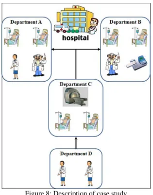
End5. CASE STUDY OF HOSPITAL SYSTEM 5.1. Case Study description
Figure 8: Description of case study
For this case study, we can see the figure 8. There are four independent departments in a hospital, which have six resources (A1, A2, B1, B2, C and D). These re-sources can achieve several activities like diagnosing, magnetic resonance imaging (MRI), operating and so on. Since the MRI machine located in department C is very
expensive, all the departments use it as a shared re-source.
The detail of resources in these four departments can be found in table 1.
Resource Activity Colour Capability Cost A1 Diagnosis 1 1 A2 Prescription 1 1 B1 Diagnosis 1 1 B2 Operate 1 1 Prescription 1.5 2 C MRI 1 1 D Control 1 1
Table 1: Resources in all departments
There are totally six resources, A1, A2, B1, B2, C and D. Each machine can achieve several activities with differ-ent capabilities and costs. The indicated cost is based on the hour cost of a machine. For instance, an operation with a predicted processing time of 12 units, requiring the “prescription” activity, it can be achieved by chine A2 after 12 time units with a cost of 12, by ma-chine B2 after 18 units with a cost of 24. We also sup-pose that the dispatching rule used for resource man-agement is FIFO (first in first out).
In each shop there are several orders from the patients, we consider them as care orders (CO). The detail charac-teristics of all care orders are given in table 2. COA1 means the first care order of department A. Because of
the specialization of medical industry, we suppose that all the care orders are required to satisfy their due date firstly. If the due date has already respected, the se-quence of care orders will be followed the low cost strat-egy. Order Objec-tive Quan-tity Order date Due date Rout-ing COA1 delay 1 1 7 2 COA2 delay 1 2 9 1 COB1 delay 1 2 11 2 COB2 delay 1 3 9 3 COC1 delay 1 2 6 4 COD1 delay 1 5 7 5
Table 2: Orders in all departments
Care orders follow the linear routings defined in table 3. An activity has to be performed on each patient depend-ing on its routdepend-ing. The routdepend-ing is a linear sequence of operations.
Routing Operation Activity Operation time 1 1 Diagnosis 2 2 Prescription 2 2 1 Diagnosis 2 2 MRI 2 3 1 Diagnosis 2 2 Operate 2 4 1 MRI 3 5 1 Control 2 Table 3: Routing
Each operation can be achieved by one or more ma-chines (maybe mama-chines with operators or doctors). Each machine has one or more competencies on several opera-tions but cannot have two competencies on the same operation nor execute different operations at the same time. The competencies of different machines on the same operation could be different. As a consequence, the processing time of one operation varies according to the competency of the chosen machines. Totally, a routing can have different processing time and related costs de-pending on the performance of the chosen machine on related activities. The predicted time of an activity is calculated by the best performing machines that can pro-cess the operation.
In order to keep the case simple and understandable, we assume that no transport time for patients between dif-ferent departments. For machines, no set-up time is con-sidered. Once an operation has started on a machine, it will finish on the same one. The disturbances frequency of machines is low during processing operation, and there is no closure time for the machines. One machine only has three possible statues: available, in processing, or in failure after a disturbance. We use figure 9 to give
an intuitive description of the orders from all the de-partments.
Figure 9: Diagram for orders
5.2. Case Study modelization
First of all, we build a DSCEP framework for the exam-ple in figure. 10. The normal customer (producer) agents are hidden in this figure. The direct connections in the figure are working through the communication bus.
Figure 10: DSCEP framework for example
Figure 11: Scheduling for shared resource This case study requires negotiation between roots SCEP models A, B and internal SCEP model C for the shared resource C. The virtual producer agents MRI in root SCEP models A and B send the wished positions of ob-ject COA1.2 “([3, 5], 0)” and COB1.2 “([4, 6], 0)” to the virtual customer agents A and B in internal SCEP model C. The local customer agents in internal SCEP model C send the wished position of object COC1.1 “([2, 5], 0)”
to the producer agent MRI. The producer agent MRI finds a conflict here. Based on the FIFO rule it schedules the orders and sends the effective positions of these four objects back: COA1.2 ([5, 7], C) to SCEP model A, COB1.2 ([7, 9], C) to SCEP model B, COC1.1 ([2, 5], C) to the local customer agents. Figure 11 give the detail scheduling process of resource C.
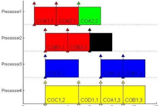
For the shared resource D in department D, we follow the same scheduling process. After all the scheduling process is finished, we can see the final scheduling result in figure 12.
Fig 12: Scheduling result for all resources
6. CONCLUSION
We introduce DSCEP framework in this communication, aiming at solving shared resource problems in complex system. We adopt a simple example in hospital systems to illustrate the DSCEP framework, which could help multiple users to schedule their local resource and also support sharing resource.
Indeed, there are some hypotheses in our illustration such as: only one resource is shared in the framework; the disturbances of the resources are set to low; the scheduling rule is limited to FIFO and so on. In the fu-ture we will continue discuss the scheduling behavior of DSCEP framework with multi shared resources in virtual enterprise. The further work may also help to fit more actual situations in different industries and lead to an automatic software application based on DSCEP frame-work.
REFERENCES
Archimede, B., and T. Coudert, 2001. Reactive schedul-ing usschedul-ing a multi-agent model: the SCEP frame-work. Engineering Application of Artificial
Intelli-gence, 14, p. 667-683.
Balaji, P.G., and D. Srinicasan, 2010. An introduction to multi-agent systems. Studies in Computational
Intel-ligence, 310, p. 1-27.
Blazewicz, J., K.H. Ecker, E. Pesch, G. Schmidt, and J. Weglarz, 2001. Scheduling Computer and
Manufac-turing Processes, Springer, Berlin.
Dechter, R., 2003. Constraint Processing. Morgan Kaufmann, San Francisco.
Ennigrou, M., and K. Ghedira, 2008. New local diversi-fication techniques for flexible job shop scheduling problem with a multi-agent approach. Autonomous
Agents and Multi-Agent Systems, 17(2), pp.
270-287.
Galvin, S., 1994. Operating system concepts. Distributed
file systems, 17. Addison-Wesley Publishing
Com-pany.
Kouider, A., and B. Bouzouia, 2012. Multi-agent job shop scheduling system based on co-operative ap-proach of idle time minimization. International
Journal of production Research, 50 (2), p. 409-424.
Le, S., and R. Boyd, 2007. Evolutionary Dynamics of the Continuous Iterated Prisoner's Dilemma. Journal
of Theoretical Biology, 245, p. 258–267.
Molina, A., and J.M. Sanchez, 1998. The virtual enter-prise. Handbook of life cycle engineering: concepts,
models, and technologies, 3, p. 59-89.
Nejad, H.T.N., N. Sugimura, and K. Iwamura, 2011. Agent-based dynamic integrated process planning scheduling in flexible manufacturing systems.
Inter-national Journal of production Research, 49 (5), p.
1373-1389.
Passos, C.A.S., V.M. Iha, and R.B. Dominiquini, 2010. A Multi-Agents Approach to Solve Job Shop Scheduling Problems Using Metaheuristics. 5th
Conference on Management and Control of Produc-tion and Logistic.
Shen, W., L. Wang, and Q. Hao, 2006. Agent-based dis-tributed manufacturing process planning and sched-uling: A state-of-the-art survey. IEEE Transactions
on Systems, Man, and Cybernetics-Part C: Applica-tions and Reviews, 36 (4), p. 563-577.
Xiang, W., and H.P. Lee, 2008. Ant colony intelligence in multi-agent dynamic manufacturing scheduling.
Engineering Application of Artificial Intelligence,
21 (1), p. 73-85.
Xu, J., B. Archimede, and A. Letouzey, 2011. Applica-tion of using SCEP model for distributed scheduling with shared resources in hospital system. Emerging
Technologies & Factory Automation (ETFA 2011), IEEE 16th Conference.