HAL Id: hal-00495969
https://hal.archives-ouvertes.fr/hal-00495969
Submitted on 29 Jun 2010
HAL is a multi-disciplinary open access
archive for the deposit and dissemination of
sci-entific research documents, whether they are
pub-lished or not. The documents may come from
teaching and research institutions in France or
abroad, or from public or private research centers.
L’archive ouverte pluridisciplinaire HAL, est
destinée au dépôt et à la diffusion de documents
scientifiques de niveau recherche, publiés ou non,
émanant des établissements d’enseignement et de
recherche français ou étrangers, des laboratoires
publics ou privés.
Modelling Saliency Awareness for Objective Video
Quality Assessment
Ulrich Engelke, Marcus Barkowsky, Patrick Le Callet, Hans-Jürgen Zepernick
To cite this version:
Ulrich Engelke, Marcus Barkowsky, Patrick Le Callet, Hans-Jürgen Zepernick. Modelling Saliency
Awareness for Objective Video Quality Assessment. International Workshop on Quality of Multimedia
Experience (QoMEX), Jun 2010, Trondheim, Norway. �hal-00495969�
MODELLING SALIENCY AWARENESS FOR OBJECTIVE VIDEO QUALITY ASSESSMENT
Ulrich Engelke
†, Marcus Barkowsky
∗, Patrick Le Callet
∗, and Hans-J¨urgen Zepernick
††
Blekinge Institute of Technology, PO Box 520, 372 25 Ronneby, Sweden
∗
IRCCyN UMR no 6597 CNRS, Ecole Polytechnique de l’Universite de Nantes,
rue Christian Pauc, La Chantrerie, 44306 Nantes, France
ABSTRACTExisting video quality metrics do usually not take into con-sideration that spatial regions in video frames are of vary-ing saliency and thus, differently attract the viewer’s atten-tion. This paper proposes a model of saliency awareness to complement existing video quality metrics, with the aim to improve the agreement of objectively predicted quality with subjectively rated quality. For this purpose, we conducted a subjective experiment in which human observers rated the an-noyance of videos with transmission distortions appearing ei-ther in a salient region or in a non-salient region. The mean opinion scores conſrm that distortions in salient regions are perceived much more annoying. It is shown that application of the saliency awareness model to two video quality metrics considerably improves their quality prediction performance.
Index Terms— Video quality metrics, visual saliency, eye
tracking, subjective quality experiment. 1. INTRODUCTION
Advanced communication networks facilitate the transition from traditional voice services to multimedia services, includ-ing packet based video streaminclud-ing over IP. This is also en-abled through contemporary video coding standards, such as H.264/AVC [1], which allows for encoding at signiſcantly lower bit rates than its predecessors, while maintaining the level of visual quality. However, the limited bandwidths in the networks and the strong signal compression result in the video content being highly prone to visual distortions through bit errors and packet loss during transmission. For service providers it is of vital importance to objectively measure the perceptual impact of these distortions to provide a certain level of Quality of Experience (QoE) to the end user. For this reason there has been an increased effort in recent years to develop objective image and video quality measures.
Earlier visual quality metrics did not take into account that visual content usually exhibits regions of varying saliency, drawing the viewer’s visual attention (VA) to different de-grees. More recently, however, there have been several stud-ies in which spatial saliency has been incorporated into still image quality metrics to improve quality prediction perfor-mance [2–5]. However, there has been only little efforts to
incorporate visual saliency into video quality metrics (VQM). This is somewhat surprising, as the effect of saliency driven attention [6] on the perception of distortions is expected to be particularly high in video signals, where the visual scene changes continuously, unlike with still images, where the vi-sual scene is static. In [7] and [8] objective saliency maps have been used in a pooling stage of video quality metrics. Both works rely on a possibly inaccurate prediction of saliency by an objective model and no qualitative or quantitative anal-ysis has been provided regarding the impact of saliency on the perceived annoyance of localised distortions.
In this paper, we aim to improve the quality prediction performance of a contemporary VQM, the temporal trajectory aware video quality measure (TetraVQM) [9], and the well known peak signal-to-noise ratio (PSNR) [10], by adding a simple saliency model. For this purpose, we used eye tracking data from a task-free experiment as a ground truth to identify saliency in a number of videos. We then introduced packet loss into the bit stream of the videos to create localised dis-tortions appearing either in a salient region or a non-salient region. In a second subjective experiment, a number of ob-servers was then asked to rate the annoyance of the distortions in the videos. The mean opinion scores (MOS) show that the annoyance of the distortions depends indeed strongly on the saliency of the region that they appear in. Having this knowl-edge, we develop a model of saliency awareness and evaluate its effectiveness by applying it to TetraVQM and PSNR, with the aim to improve the agreement of the objectively predicted quality with the MOS from the subjective experiment.
This paper is organised as follows. Section 2 explains the subjective experiment that we conducted. Section 3 reviews the video quality metric TetraVQM. The saliency awareness modelling is presented in Section 4. A performance evalua-tion of the saliency aware metrics is discussed in Secevalua-tion 5. Conclusions are ſnally drawn in Section 6.
2. SUBJECTIVE EXPERIMENT
We conducted a subjective experiment at the University of Nantes, France, to obtain a ground truth for the perceived an-noyance of packet loss distortions. The experiment is dis-cussed in detail in [11] and is summarised in the following.
2.1. Creation of distorted test sequences
We considered 30 reference videos in standard deſnition (SD) format, provided by the Video Quality Experts Group (VQEG) [12], of which we selected 20 sequences for the experiment with respect to the saliency and the spatial and temporal char-acteristics of the content. The latter were quantiſed using spatial information (SI) and temporal information (TI) indi-cators [13]. The saliency in each sequence was identiſed us-ing gaze patterns from an earlier eye trackus-ing experiment [14] where the 30 sequences were presented to 37 participants un-der task free condition. The gaze patterns of all observers were post-processed into saliency maps. An example of a reference sequence frame and an overlayed saliency map is shown in Fig. 1(a) and Fig. 1(b), respectively.
We encoded the sequences in H.264/AVC format [1] us-ing the JM 16.1 reference software [15]. The sequences were encoded with a constant quantization parameter QP=28 and in High proſle with an IBBPBBP... GOP structure of two dif-ferent lengths; 30 frames (GOP30) and 10 frames (GOP10). The frame rate was set to 25 and thus, the GOP lengths corre-spond to 1.2 sec and 0.4 sec, respectively. All sequences were shortened to 150 frames, corresponding to 6 sec duration.
We adapted the Joint Video Team (JVT) loss simulator [16] to introduce packet loss into the H.264/AVC bit stream. The packet loss was introduced into a single I frame in each sequence resulting in error propagation until the next I frame, due to the inter-frame prediction of the P and B frames. Thus, the two GOP lengths, 30/10 frames, relate to the maximum error propagation lengths 1.2/0.4 sec. To have better control regarding the location and extent of the loss patterns we chose a ſxed number of 45 macro blocks (MB) per slice. Given that SD video has a resolution of720 × 576 pixels, corresponding to45 × 36 MB, each slice represents exactly one row of MB. We introduced packet loss into the reference sequences, SEQ𝑅, such as that the distortions appear either in a salient
region or non-salient region. In particular, we created dis-torted sequences with packet loss introduced in 5 consecutive slices centered around a highly salient region of an I frame. We then created a corresponding sequence with 5 consec-utive lost slices introduced into a non-salient region of the same I frame. We created such two sequences for both the GOP30 and GOP10 coded sequences. The subsets of dis-torted sequences are in the following referred to as SEQ𝑆,0.4,
SEQ𝑁,0.4, SEQ𝑆,1.2, and SEQ𝑁,1.2, where0.4 relates to error
propagation length for GOP10 and, accordingly,1.2 relates to GOP30. The indices𝑆 and 𝑁, respectively, denote the salient
and the non-salient region. An example of a frame containing distortions in the salient region and in the non-salient region is shown in Fig. 1(c) and Fig. 1(d), respectively.
2.2. Experiment details
The experiment was designed according to ITU Rec. BT.500 [17]. The videos were presented on a LVM-401W full HD
(a) (b)
(c) (d)
Fig. 1. Frame 136 of the video sequence ’Kickoff’: (a) ref-erence video, (b) saliency information, (c) distortions in the salient region, (d) distortions in the non-salient region. screen by TVlogic with a size of 40" and a native resolution of1920 × 1080 pixels. A mid-grey background was added to the SD test sequences to be displayed on the HD screen. The observers were seated at a distance of about 150 cm cor-responding to six times the height of the used display area.
Thirty non-expert observers participated in the experiment (10 female, 20 male) with an average age of about 23 years. Prior to each experiment, the visual accuracy of the partici-pants was tested using a Snellen chart and colour deſciencies were ruled out using the Ishihara test. The participants were presented the 100 test sequences (20 reference, 80 distorted) in a pseudo random order with a distance between the same content of at least 5 presentations. The sequences were pre-sented using a single stimulus method.
The 5-point impairment scale [17] was used to assess the annoyance of the distortions in the sequences. Here, the ob-servers assigned one of the following adjectival ratings to each of the sequences: ’Imperceptible (5)’, ’Perceptible, but not annoying (4)’, ’Slightly annoying (3)’, ’Annoying (2)’, and ’Very annoying (1)’. The impairment scale was given the preference over the quality scale (also deſned in [17]), as the rating ’Imperceptible’ directly allows to identify whether or not participants actually detected the distortions. The partici-pants were shown 6 training sequences to get a feeling for the distortions to be expected in the test sequences.
2.3. Experiment outcomes
The 30 subjective scores for each sequence are averaged into MOS. Corresponding to the subsets of sequences we deſne MOS subsets MOS𝑅, MOS𝑆,0.4, MOS𝑁,0.4, MOS𝑆,1.2, and
1 2 3 4 5 6 7 8 9 10 11 12 13 14 15 16 17 18 19 20 1 1.5 2 2.5 3 3.5 4 4.5 5
Video sequence number
MOS
MOSR MOSS,0.4 MOSN,0.4 MOSS,1.2 MOSN,1.2
Fig. 2. MOS and standard errors for all 20 sequence contents in each subset. R N/0.4 N/1.2 S/0.4 S/1.2 1 2 3 4 5 MOS subset
Fig. 3. MOS averaged over all 20 sequences for each subset.
MOS𝑁,1.2. The MOS subsets, including the standard errors,
are shown in Fig. 2 for all 20 contents. It can be observed that the hierarchy of MOS between the subsets is almost ex-clusively the same for all sequences. The reference sequences SEQ𝑅 always received the highest scores, followed by
SEQ𝑁,0.4, SEQ𝑁,1.2, SEQ𝑆,0.4, and SEQ𝑆,1.2.
The MOS for each of the subsets, averaged over all 20 contents, is shown in Fig. 3. It can be seen that the MOS difference between sequences with distortions in the salient region and in the non-salient region is signiſcantly larger as compared to the MOS difference between sequences with long and short distortions. This indicates that the observers distin-guish annoyance levels more pronounced with respect to the saliency of the distortion region as compared to the distor-tion duradistor-tion. It is particularly worth noting that SEQ𝑁,1.2
re-ceived an average MOS that is 1.02 higher than for SEQ𝑆,0.4,
even though the distortion in the non-salient region is three times longer than the distortion in the salient region.
In summary, the MOS show strong evidence that the vi-sual saliency plays a vital role in judging the perceived an-noyance of packet loss degradations. As such, one can expect an improvement in quality prediction performance by incor-porating saliency information into VQM.
3. TETRAVQM
TetraVQM is an objective quality algorithm that is particu-larly well suited for the enhancement with visual saliency be-cause it already contains several steps that are motivated by the human visual system. It has been designed for the pre-diction of video quality in multimedia scenarios including the typical artifacts that occur in packet loss situations.
The TetraVQM algorithm uses the reference and the de-graded video to predict the perceived quality. Its main focus is on temporal issues, e.g. the misalignment of the two video sequences, frame freezes and skips, frame rate reduction, in-ƀuence of scene cuts, and, in particular, the tracking of the visibility of distorted objects. The processing starts with the spatial, temporal, and color alignment of the two input videos. For each aligned image, a spatial distortion map is created which identiſes the position and the severity of the degrada-tions using the simple mean squared error (MSE). A human observer perceives the video sequence as a continuous stream of information rather than image by image. For example, it was shown that the perceived severity of artifacts depends on the duration that the artifact is seen. Short distortions are less annoying than longer distortions. However, degradations which move together with an object are perceived as long last-ing object degradations rather than several isolated momen-tary points of distortions. Therefore, TetraVQM estimates the object motion and keeps track of the degradations over time. Each initial distortion map is then modiſed to account for the temporal visibility of the artifacts.
The spatial summation is performed by applying a ſlter that is based on the distribution of the cones in the fovea. Cur-rently, the assumption is used that the viewer focuses on the point of the maximum perceived degradation. This was pre-viously seen as the focal point of the observer. Thus, it is straightforward to improve the algorithm by applying a more sophisticated approach that uses the visual saliency. In this paper a ſrst step towards this goal is presented.
A scatter plot of TetraVQM versus the MOS from the ex-periment we conducted is presented in Fig. 4. In this ſgure, the sequences corresponding to the four different subsets of distortions (SEQ𝑆,0.4, SEQ𝑁,0.4, SEQ𝑆,1.2, SEQ𝑁,1.2) are
il-lustrated using different markers. In addition, cluster means (𝜇𝑆,0.4,𝜇𝑁,0.4, 𝜇𝑆,1.2, 𝜇𝑁,1.2) are provided for all subsets.
The scatter plot highlights that TetraVQM accounts for the temporal duration of the distortions but not for the saliency of the distortion region. The latter is evident given the big gap in MOS and the small gap in TetraVQM between the sequences with distortions in the salient and non-salient region.
4. SALIENCY AWARENESS
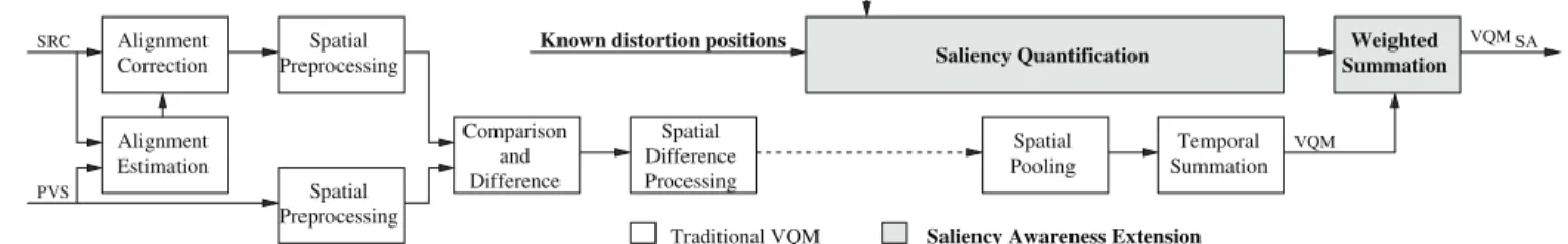
An overview of the saliency awareness model applied to a VQM is depicted in Fig. 5. The idea is to extend a traditional VQM (white blocks) with the saliency awareness model (grey
Alignment
Correction PreprocessingSpatial
SRC Alignment Estimation Comparison and Difference Spatial Difference Processing Spatial
Pooling SummationTemporal
Traditional VQM
PVS Spatial
Preprocessing
Known distortion positions
Saliency measured in subjective experiment
Weighted Summation
Saliency Awareness Extension Saliency Quantification
VQM
SA VQM
Fig. 5. Overview of the extension of a traditional VQM with the proposed saliency awareness model.
1 2 3 4 5 1 2 3 4 5 TetraVQM MOS SEQS,0.4 μS,0.4 SEQN,0.4 μN,0.4 SEQS,1.2 μS,1.2 SEQN,1.2 μN,1.2
Fig. 4. Scatter plot of TetraVQM versus MOS, highlighting the four subsets of distortions and their mean values. blocks), without having to change the actual VQM. As can be seen from Fig. 5, the VQM is computed in its regular way and then subjected to a weighted summation with respect to the saliency of the distorted image content as follows
VQMSA = VQM − 𝛼 ⋅ S (1)
where S denotes the saliency information. The idea behind Eq. 1 is to add a negative offsetΔ = −𝛼 ⋅ S to the VQM with respect to the amount of saliency information in the region where the distortions appear. This is based on the assump-tion, that distortions in a more salient region are perceived as more annoying and as such, will receive a lower subjective quality score. In this respect, the parameter S represents the saliency within the distortion region of a particular video and thus, regulates the relative magnitude of the offset between different contents. The parameter𝛼 regulates the general
de-gree with which the offset is performed and needs to be opti-mised for any particular VQM.
In a practical application, the distorted regions can be de-tected using distortion maps that are readily available in most traditional VQM. In this work, however, we use the perfect knowledge of the distortion regions due to the controlled cre-ation of the test videos. To avoid potential saliency prediction errors from objective methods, that would subsequently result in errors in the saliency awareness model, we use in this work the saliency maps created from the gaze patterns from the eye tracking experiment (see Section 2.1).
The model outlined here is considered to be generally ap-plicable to any VQM that does not take into account visual saliency. In the following we present two different saliency quantiſcation methods that were found to signiſcantly im-prove the quality prediction performance of both TetraVQM and PSNR.
4.1. Saliency quantiſcation method 1
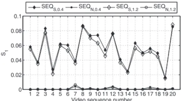
The saliency awareness model using this ſrst saliency quan-tiſcation method is in the following referred to as model M1. This method takes into account, that the saliency within the distortion region varies between different videos. For this rea-son, the saliency in the distorted regions is quantiſed using the saliency maps created from the gaze patterns. An exam-ple of a saliency map, corresponding to the frame presented in Fig. 1, is presented in Fig. 6. The distortion regions are highlighted for the salient region (white grid) and for the non-salient region (grey grid). The mean saliency is then com-puted over the whole distortion region as follows
S1= (𝑙𝑖𝑚 1 𝑏− 𝑙𝑖𝑚𝑡)(𝑙𝑖𝑚𝑟− 𝑙𝑖𝑚𝑙) 𝑙𝑖𝑚∑𝑡 𝑚=𝑙𝑖𝑚𝑏 𝑙𝑖𝑚∑𝑟 𝑛=𝑙𝑖𝑚𝑙 S(𝑚, 𝑛) (2) where𝑙𝑖𝑚𝑏, 𝑙𝑖𝑚𝑡,𝑙𝑖𝑚𝑙, and𝑙𝑖𝑚𝑟, respectively, denote the
limits of the distortion region on the bottom, top, left, and right. The temporal pooling calculates the mean over all de-graded frames. The saliency magnitudes S1for all sequences
are shown in Fig. 7. One can see that the sequences SEQ𝑆,0.4
and SEQ𝑆,1.2 contain a higher amount of saliency as
com-pared to SEQ𝑁,0.4 and SEQ𝑁,1.2, however, the amount of
saliency is not constant between the different sequences. 4.2. Saliency quantiſcation method 2
The saliency awareness model using this saliency quantiſca-tion method is in the following referred to as model M2. This method does not distinguish between as many saliency levels as M1 does, but rather distinguishes only between two cases; salient region or non-salient region. This can be realised with a threshold algorithm as follows
S2= 1 for S1≥ 𝜏 (3)
S2= 0 for S1< 𝜏
1 720 1 576 0 0.2 0.4 0.6 0.8 1 1.2 1.4 1.6
Fig. 6. Saliency map of frame 136 of the video ’Kickoff’ with distortion regions highlighted for the salient region (white grid) and the non-salient region (grey grid).
1 2 3 4 5 6 7 8 9 10 11 12 13 14 15 16 17 18 19 20 0 0.02 0.04 0.06 0.08 0.1
Video sequence number
S1
SEQS,0.4 SEQN,0.4 SEQS,1.2 SEQN,1.2
Fig. 7. Saliency quantiſcation S1for all 20 sequence contents
in each subset.
Considering the results presented in Fig. 7, we deſne a thresh-old of𝜏 = 0.01 which separates the classes of saliency and
non-saliency in the distorted image content. As such, the VQM scores for the sequences SEQ𝑆,0.4 and SEQ𝑆,1.2
re-ceive the same offset, whereas the VQM scores for the se-quences SEQ𝑁,0.4and SEQ𝑁,1.2remain unaltered.
5. EVALUATION
The quality prediction performance of the metrics TetraVQM and PSNR is evaluated using three performance indicators; the root mean squared error (RMSE), the Pearson linear corre-lation coefſcient𝜚𝑃, and the Spearman rank order correlation
𝜚𝑆. Prior to calculating the RMSE, a linear ſt is applied in
or-der to align the VQM output to the subjective rating scale. For the model enhancements presented in the previous Section, optimal parameters𝛼𝑜𝑝𝑡are determined with respect to
min-imising RMSE using an exhaustive search. For TetraVQM, the relation between the 𝛼 and the RMSE is presented in
Fig. 8 and the correspondence between𝛼 and the correlation
coefſcients is given in Fig. 9. The minimum RMSE and the maximum𝜚𝑃 and𝜚𝑆are highlighted in the respective ſgures.
The performance values are summarised in Tab. 1 for the VQMs and their proposed enhancements as in TetraVQMM1, TetraVQMM2 and PSNRM1, PSNRM2. The performance results of TetraVQM and PSNR without the proposed
en-Table 1. Optimised parameters𝛼𝑜𝑝𝑡 and quality prediction
performance indicators for TetraVQM and PSNR.
Metric 𝛼𝑜𝑝𝑡 RMSE Pearson Spearman
TetraVQM N/A 0.702 0.522 0.536 TetraVQMM1 28.15 0.447 0.84 0.835 TetraVQMM2 2.41 0.316 0.923 0.888 PSNR N/A 0.75 0.414 0.451 PSNRM1 418.61 0.465 0.825 0.83 PSNRM2 35.08 0.332 0.915 0.88
hancements indicate that these metrics are unable to predict the results of this particular subjective experiment consist-ing of an isolated distortion type. When comparconsist-ing between TetraVQM and PSNR, it can be observed that TetraVQM con-sistently performs better than PSNR.
The results show that for both models M1 and M2, the RMSE can be largely decreased and the correlation coefſ-cients can be largely increased. The model M2 achieves better results than model M1, even though M2 does not distinguish saliency levels between the distortion regions of the different sequences, but instead uses a constant offset for SEQ𝑆,0.4and
SEQ𝑆,1.2. It should be noted that for𝜚𝑆 of model M2, the
maximum coincides with the𝛼2for which the TetraVQMM2
of all sequences SEQ𝑆,0.4 and SEQ𝑆,1.2 are shifted below
the TetraVQMM2 of the sequences SEQ𝑁,0.4and SEQ𝑁,1.2.
Thus, the rank order correlation of the objective quality scores with MOS is highest when all sequences with distortions in the salient regions are rated lower than the worst sequence with distortions in the non-salient region. This observation is in line with the conclusions drawn from the MOS of the subjective experiment (see Section 2.3 and Fig. 2).
Scatter plots of TetraVQMM1 and TetraVQMM2 are pre-sented in Fig. 10 after deploying a linear mapping to the MOS. The scatter plot for TetraVQMM2 shows two distinct point clouds for the two classes salient and non-salient which par-tially corresponds to the situation seen in Fig. 2. This is re-markable because the optimization has been performed on the RMSE value and not on the correlation coefſcients and thus, it is not an artifact of the training. Nevertheless, it should be noted that the values provided in Tab. 1 provide an upper bound of the expected performance because the same subjec-tive data has been used for training as well as for evaluation.
6. CONCLUSIONS
In this paper, we proposed two models of saliency aware-ness for video quality metrics. The modelling was conducted based on subjective ground truth for both the saliency infor-mation and for the annoyance of the packet loss distortions. Application of the models to VQM reveals that the resulting saliency aware metrics show strong improvement in quality
0 20 40 60 0.3 0.4 0.5 0.6 0.7 α1 RMSE RMSE RMSEmin 0 1 2 3 0.3 0.4 0.5 0.6 0.7 α2 RMSE RMSE RMSEmin
Fig. 8. Root mean squared error (RMSE) versus𝛼1and𝛼2.
0 20 40 60 0.5 0.6 0.7 0.8 0.9 1 α1 Correlation ρP ρP,max ρS ρS,max 0 1 2 3 0.5 0.6 0.7 0.8 0.9 1 α2 Correlation ρP ρP,max ρS ρS,max
Fig. 9. Pearson correlations (𝜚𝑃) and Spearman correlations
(𝜚𝑆) versus𝛼1and𝛼2. 1 2 3 4 5 1 2 3 4 5 TetraVQMM1 MOS Videos Linear fit CI (95%) 1 2 3 4 5 1 2 3 4 5 TetraVQMM2 MOS Videos Linear fit CI (95%)
Fig. 10. Scatter plots of TetraVQMM1 and TetraVQMM2 versus MOS, including 95% conſdence intervals (CI). prediction performance, as compared to the original metrics.
Further studies are planned to improve the implementa-tion of saliency informaimplementa-tion in the objective measurement of video quality by incorporating the saliency information di-rectly into the algorithmic processing. This allows for a more comprehensive approach as the measured spatio-temporally localised visual degradations can be weighted immediately with the saliency information.
7. REFERENCES
[1] International Telecommunication Union, “Advanced video coding for generic audiovisual services,” Rec. H.264, ITU-T, Nov. 2007.
[2] U. Engelke and H.-J. Zepernick, “A framework for opti-mal region-of-interest based quality assessment in wire-less imaging,” Journal of Electronic Imaging, Special
Section on Image Quality, vol. 19, no. 1, 011005, Jan.
2010.
[3] H. Liu and I. Heynderickx, “Studying the added value of visual attention in objective image quality metrics based on eye movement data,” in Proc. of IEEE Int. Conf. on
Image Processing, Nov. 2009.
[4] A. K. Moorthy and A. C. Bovik, “Visual importance pooling for image quality assessment,” IEEE Journal of
Selected Topics in Signal Processing, vol. 3, no. 2, pp.
193–201, Apr. 2009.
[5] A. Ninassi, O. Le Meur, P. Le Callet, and D. Barba, “Does where you gaze on an image affect your percep-tion of quality? applying visual attenpercep-tion to image qual-ity metric,” in Proc. of IEEE Int. Conf. on Image
Pro-cessing, Oct. 2007, vol. 2, pp. 169–172.
[6] L. Itti, C. Koch, and E. Niebur, “A model of saliency-based visual attention for rapid scene analysis,” IEEE
Trans. on Pattern Analysis and Machine Intelligence,
vol. 20, no. 11, pp. 1254–1259, Nov. 1998.
[7] J. You, A. Perkis, M. Hannuksela, and M. Gabbouj, “Perceptual quality assessment based on visual attention analysis,” in Proc. of ACM Int. Conference on
Multime-dia, Oct. 2009, pp. 561–564.
[8] X. Feng, T. Liu, D. Yang, and Y. Wang, “Saliency based objective quality assessment of decoded video affected by packet losses,” in Proc. of IEEE Int. Conf. on Image
Processing, Oct. 2008, pp. 2560–2563.
[9] M. Barkowsky, J. Bialkowski, B. Eskoſer, R. Bitto, and A. Kaup, “Temporal trajectory aware video quality mea-sure,” IEEE Journal of Selected Topics in Signal
Pro-cessing, vol. 3, no. 2, pp. 266–279, Apr. 2009.
[10] NTIA / ITS, “A3: Objective Video Quality Measure-ment Using a Peak-Signal-to-Noise-Ratio (PSNR) Full Reference Technique,” ATIS T1.TR.PP.74-2001, 2001. [11] U. Engelke, P. Le Callet, and H.-J. Zepernick, “Linking
distortion perception and visual saliency in H.264/AVC coded video containing packet loss,” in Proc. of
SPIE/IEEE Int. Conf. on Visual Communications and Image Processing, July 2010.
[12] Video Quality Experts Group, “VQEG FTP ſle server,” ftp://vqeg.its.bldrdoc.gov/, 2009.
[13] International Telecommunication Union, “Subjective video quality assessment methods for multimedia appli-cations,” Rec. P.910, ITU-T, Sept. 1999.
[14] F. Boulos, W. Chen, B. Parrein, and P. Le Callet, “A new H.264/AVC error resilience model based on regions of interest,” in Proc. of Int. Packet Video Workshop, May 2009.
[15] Heinrich Hertz Institute Berlin, “H.264/AVC reference software JM 16.1,” http://iphome.hhi.de/suehring/tml/, 2009.
[16] Joint Video Team (JVT) of ISO/IEC MPEG and ITU-T VCEG, “SVC/AVC Loss Simulator,” http://wftp3.itu.int/av-arch/jvt-site/2005 10 Nice/, 2005.
[17] International Telecommunication Union, “Methodology for the subjective assessment of the quality of television pictures,” Rec. BT.500-11, ITU-R, 2002.