Titre:
Title:
Automatic incorporation of circular riverbank failures in two-
dimensional flood modeling
Auteurs:
Authors: Ismail Ouchebri et Tew-Fik Mahdi
Date: 2020
Type:
Article de revue / Journal articleRéférence:
Citation:
Ouchebri, I. & Mahdi, T.-F. (2020). Automatic incorporation of circular riverbank failures in two-dimensional flood modeling. Canadian Journal of Civil Engineering. doi:10.1139/cjce-2019-0670
Document en libre accès dans PolyPublie
Open Access document in PolyPublieURL de PolyPublie:
PolyPublie URL: https://publications.polymtl.ca/5478/
Version: Version finale avant publication / Accepted version Révisé par les pairs / Refereed Conditions d’utilisation:
Terms of Use: Tous droits réservés / All rights reserved
Document publié chez l’éditeur officiel
Document issued by the official publisher
Titre de la revue:
Journal Title: Canadian Journal of Civil Engineering Maison d’édition:
Publisher: Canadian Science Publishing URL officiel:
Official URL: https://doi.org/10.1139/cjce-2019-0670 Mention légale:
Legal notice:
Ce fichier a été téléchargé à partir de PolyPublie, le dépôt institutionnel de Polytechnique Montréal
This file has been downloaded from PolyPublie, the institutional repository of Polytechnique Montréal
1
AUTOMATIC INCORPORATION OF RIVERBANK FAILURES IN
TWO-1
DIMENSIONAL FLOOD MODELING
2
Ouchebri, Ismail1; Mahdi, Tew-Fik2 3
1 Ph.D Student, Département des génies Civil, Géologique et des Mines (CGM), École Polytechnique de 4
Montréal, C.P. 6079, succursale Centre-Ville, Montréal, QC H3C 3A7, Canada. Email: 5
2 Professor, Département des génies Civil, Géologique et des Mines (CGM), École Polytechnique de 7
Montréal, C.P. 6079, succursale Centre-Ville, Montréal, QC H3C 3A7, Canada (Corresponding author). 8
Email: [email protected]
9
Abstract
10
Riverbanks undergo changes caused not only by river hydraulics, mainly sediment erosion and deposition 11
processes, but also by the possible landslides that eventually change the channel bank profiles. Those 12
failures are an important form of alluvial channel adjustments but are usually difficult to include during 13
morphodynamic modeling. This paper proposes a novel approach combining a 2D depth-averaged 14
hydrodynamic, sediment transport and mobile-bed model, SRH-2D, a limit equilibrium slope-stability 15
model, BISHOP, and a bank failure sediment redistribution submodel, REDISSED, into a fully automatic 16
and continuous dynamic simulation to predict vertical bed and lateral bank changes for a river reach 17
undergoing exceptional flooding. The in-stream vertical fluvial changes predicted with the SRH-2D model 18
will be automatically used to update the riverbank geometry profile by profile and assess their 19
geotechnical stability to rotational slip failures with a developed slope-stability model based on Bishop’s 20
simplified method. A cone-shaped sliding area is defined in case the driving forces exceed the stabilizing 21
forces. All mesh nodes located within the mass wasting zone will be automatically updated, allowing a 22
new bank face form. The failed materials will be redistributed in the transect according to the geometry of 23
the landslides observed at the study site. The Outaouais River at Notre-Dame-Du Nord, Quebec, is used 24
to test the coupling procedure. Up to 100 m of bank retreat was predicted, and more than 20 cross-25
2
sections were reshaped. Typical results showing the effectiveness of the developed framework are 26
presented and discussed. 27
Author keywords
: Streambank erosion; Riverbank failure; Two-dimensional modeling; SRH-2D; 28BISHOP; Automatic coupling; Sediment redistribution. 29
Introduction
30
Rivers are dynamic systems governed by hydraulic and sediment transport processes. Over time, 31
meandering channels respond to changing conditions in the environment by modifying their cross-32
sectional and planform shapes. In fact, alluvial rivers in nature display morphological adjustments in 33
response to the exerted stresses, especially erosion, triggered by the interaction of flow and the riverbed 34
or banks. Streambank erosion is considered one of the most important processes in adjusting alluvial 35
systems (Langendoen et al. 2009). It is a natural process that occurs when the forces exerted by flowing 36
water exceed the resisting forces of the bank materials and vegetation (Simon et al. 2000). This type of 37
erosion is generally regarded as a combination of the fluvial entrainment of bank materials by flowing 38
water and the mass failure of unstable banks (ASCE Task Committee on Hydraulics 1998; Darby et al. 39
2007; Langendoen and Simon 2008). From a numerical perspective, riverbank failures are often 40
overlooked when modeling channel morphological evolution; the multidimensional hydrodynamic and bed 41
evolution models only evaluate fluvial erosion and need to be coupled with bank erosion submodels to 42
assess channel morphological adjustments evoked by riverbank geotechnical mass failures. 43
To properly examine river morphological evolution, researchers and practitioners have established a large 44
number of assumptions, developed tools and models and utilized different approaches and techniques to 45
combine both fluvial erosion and mass wasting (Lai et al. 2012; Lai et al. 2015; Langendoen et al. 2016; 46
Langendoen and Simon 2008; Mahdi and Marche 2003; Rousseau et al. 2017). Notwithstanding the 47
various employed strategies, they all aim to integrate the different physical processes responsible for 48
bank retreat into one runnable solution by coupling physical and process-based models. One of those 49
solutions consisted of combining the flowing-water and bank erosion computer models with mass failure 50
predictive models. (Mahdi and Marche 2003) were probably the first to simulate the morphologic 51
adjustment of both the bed and the banks over a long river reach (9.8 km) in a natural meandering river 52
3
system by coupling one-dimensional (1D) erosion and sediment transport model GSTARS-1D (Yang et al. 53
1998) with a bank-stability model called BISHOP to assess the circular failures of nonhomogenous 54
cohesive banks (Mahdi and Merabtene 2010; Mahdi and Marche 2003); the combined model was later 55
used to evaluate bank retreat of the river downstream of the Première Chute Dam (Mahdi 2004) in 56
Quebec and yielded a promising results. However, the mobile-bed model GSTARS-1D (Yang et al. 1998) 57
uses a simple theory in that the channel geometry adjustments can be vertical or lateral depending on the 58
minimum unit stream power theory (Yang 1976), an approach that can be used only for short- and 59
medium-term predictions (Simon et al. 2007). Similarly, (Langendoen and Simon 2008) merged an 60
unsteady one-dimensional channel evolution and physically based model called CONCEPTS 61
(Langendoen 2000) with a geotechnical submodel to simulate the streambank planar failures of 62
riverbanks over the bendway of Goodwin Creek, Mississippi, and later over two incised streams in 63
northern Mississippi, James Creek and the Yalobusha River (Langendoen et al. 2009). (Motta et al. 2012) 64
coupled the physically based algorithms of the channel evolution model CONCEPTS (Langendoen 2000) 65
with the (2D) hydrodynamic and migration RVR Meander model (Abad and Garcia 2006) to simulate 66
meander migration at the reach scale. Recently, (Motta et al. 2012) simulated bank retreat also using the 67
one-dimensional computer model CONCEPTS (Langendoen 2000) to investigate the impact of the 68
variability of erodibility parameters on the model’s lateral retreat predictions. However, CONCEPTS 69
(Langendoen 2000) and likely GSTARS-1D (Yang et al. 1998) are 1D models they do not incorporate 70
corrections for secondary currents and transversal bed slope, and hydraulics are not adequately resolved 71
to predict bank erosion. Therefore, their applicability to meander bends might underestimate the shear 72
stress along the streambank. Indeed, the increased shear stresses for the CONCEPTS (Langendoen 73
2000) model are represented by a reduction in resistance to erosion of the bank material (Langendoen 74
and Simon 2008); the model is unable to predict the increased hydraulic forces acting on the outer banks 75
caused by the helical flow patterns in the bends, which limits its applicability to only in regions where the 76
phenomena can be neglected (Lai et al. 2012). Moreover, (Abad and Garcia 2006) showed less variation 77
in predicted retreat by the one-dimensional model compared to the incorporated erodibility parameters 78
derived from streambank tests and, more importantly, stressed the need for two- or three-dimensional 79
modeling. 80
4
The coupling between riverbank mass failure algorithms and one-dimensional computer models was 81
probably the only way to account for streambank erosion as an important process of river morphological 82
adjustment, despite the simplified physically based equations implemented and the relevant assumptions 83
involved. In recent years, researchers have taken advantage of two-dimensional (2D) morphodynamic 84
numerical models to better understand the interactions between fluvial erosion and mass wasting. 85
(Rinaldi et al. 2008) enhanced our comprehension of this matter by coupling the different components of 86
bank retreat separately using the 2D depth-averaged hydrodynamic model (Deltares Delft 3D) with the 87
commercial groundwater model (GeoSlope, SEEP/W) and the bank stability analysis model (GeoSlope, 88
SLOPE/W) and applied it in a reach-scale hydraulics study within the river bend of the Cecina River, Italy. 89
Despite the overall success of highlighting the roles of fluvial erosion and mass failure driven by 90
hydrodynamic conditions and geotechnical factors, the (Rinaldi et al. 2008) approach loosely accounted 91
for feedbacks between the eroded bank and the flow and simply ignored bed-level changes. In addition, 92
the approach is computationally expensive in terms of the time needed for manual remeshing, making it 93
strictly convenient to simulate a single flood event. Recently, (Rousseau et al. 2017) developed and 94
coupled a riparian vegetation module and a geotechnical algorithm with the two-dimensional solver 95
Telemac-Mascaret (Galland et al. 1991) to predict bank retreat for a semialluvial meandering reach 96
(Medway Creek, Ontario, Canada). The study addressed the effects of plants on the mechanical 97
properties of riverbanks and evaluated the geotechnical stability of the banks independently of the 98
hydrodynamic mesh. It is among the rarest studies to include mass wasting and vegetation processes 99
over a long spatiotemporal scale. (Lai et al. 2015) coupled the deterministic bank stability and toe erosion 100
model (BSTEM) (Simon et al. 2011) developed by the National Sedimentation Laboratory to the 2D 101
depth-averaged hydraulic and sediment transport model SHR-2D (Lai 2010) to predict streambank retreat 102
and planform development. (Lai et al. 2015) evaluated the bank erosion using the near-bank bed shear 103
stress computed by SRH-2D (Lai 2010) and manually moved the mesh to account for the bank toe 104
displacement, an approach that might be very costly in terms of time needed to readjust the mesh and 105
especially, as the researchers acknowledged, the time required to update and interpolate variables. Later, 106
(Lai 2017) extended the previous moving mesh approach to the fixed mesh method and showed that it is 107
often useful to combine both approaches to improve the robustness of the numerical model and thus 108
5
accurately predict vertical stream bed changes and lateral streambank erosion for complex systems. In 109
both cases, bank geometries and their erosion are treated separately from SRH-2D (Lai 2010) 110
components. A strategy that allows adequate representation of the bank geometry is often difficult using 111
two-dimensional models that generally reduce bank profiles to a single linear segment. 112
The state-of-the-art described above presents the most recent studies coupling multiple versions of one-113
dimensional or two-dimensional models simulating both bed and bank adjustments. Most of those studies 114
are time consuming if applied on a long-reach scale. Moreover, to correctly represent bank geometry 115
within two-dimensional mobile-bed models, geotechnical evaluations are performed independently from 116
the mesh. Thus, in the case of bank retreat, the mesh needs to be readjusted manually, which makes the 117
coupling procedure strictly practical on a limited-size channel. Furthermore, since there is no consensus 118
among researchers considering the redistribution of the derived bank materials, morphodynamical studies 119
simply omit or utilize ad hoc approaches to redeposit the failed blocks (Darby and Delbono 2002; Nagata 120
et al. 2000; Pizzuto 1990). In this article, the authors aim to overcome these difficulties by developing a 121
new platform capable of the following: first, describing adequately the stratigraphy and bank geometry of 122
the cross-sections, along which slope-stability assessments are performed, in a 2D mesh without 123
necessarily needing to idealize them; second, assessing their geotechnical stability to rotational failures 124
using an automatic search routine capable of identifying the minimum factor of safety at the potentially 125
unstable riverbanks; third, and most importantly, redistributing slump blocks onto the 2D mesh based on 126
the topographic form of the failed materials in the study area while conserving the mass; and fourth, 127
simulating the feedbacks between the coupled models at each time step automatically, including the 128
mesh movement, without user intervention. The developed procedure is an easy-to-use and time-saving 129
tool for evaluating streambank retreat due to both fluvial erosion and geotechnical failure in long-reach 130
scale modeling systems. Details of the pairing scheme are described in the following sections. The model 131
is applied to the analysis of the evolution of a river reach several kilometers downstream of a dam break 132
scenario. 133
6
Overview of the model components
134
In the present modeling investigation, we combine the 2D mobile-bed model SRH-2D (Lai 2008; Lai 135
2010) with the slope stability model BISHOP (Mahdi 2004; Mahdi and Merabtene 2010) and the riverbank 136
failed materials redistribution submodel REDISSED (Mahdi 2004). In the following, the models are 137
presented first, and their coupling is then described and discussed. 138
SRH-2D Model 139
The SRH-2D (Sedimentation and River Hydraulics - Two-Dimensional) model (Lai 2008; Lai 2010) is a 140
two-dimensional flow, mobile-bed and sediment transport model developed by the U.S. Bureau of 141
Reclamation. The model is flexible; it uses an unstructured hybrid mesh numerical method that can be 142
applied to arbitrarily shaped cells. Moreover, SRH-2D solves the 2D dynamic wave equations, i.e., the 143
depth-averaged St. Venant equations, with a very robust and stable numerical scheme based on a finite 144
volume discretization. In terms of hydrodynamic modeling capabilities, SRH-2D has shown its capacities 145
for hydraulic calculations compared to Hydro_As-2D (Lavoie and Mahdi 2017) and was previously tested 146
successfully in many other studies (Lai et al. 2010; Lai et al. 2016; Moges 2010). 147
For a complete analysis within SRH-2D, the model needs a mesh generator. Since the model adopts the 148
arbitrarily shaped mesh system, any 2D mesh generator program may be used. At present, SRH-2D uses 149
the SMS model (AQUAVEO 2019) as the mesh generator and postprocessing graphical model. A typical 150
modeling consists of delimiting the initial solution domain on the SMS, defining the topographic and 151
bathymetric data, assigning the channel’s materials and boundary conditions and finally generating the 152
mesh. Within the SMS, it is possible to run SRH-2D for single simulation or to export all the simulation 153
data into files for future use, an approach that will be adopted in this study. The authors will use the 154
exported data to launch the SRH-2D processor (srh-2d). The model outputs the results files that describe 155
the time-dependent evolution of the cross-sections. Several forms of data processing can be considered. 156
BISHOP Model 157
BISHOP is a geotechnical stability analysis model developed by (Mahdi 2004) to evaluate bank profile 158
stability. The model iteratively calculates the minimum factor of safety based on Bishop's modified method 159
7
(Philiponnat and Hubert 1979); it isolates the global minimum factor of safety from all the local minima for 160
a given slope. Stability analysis is carried out based on the approach of circular failures, a type of 161
riverbank failure often noticed in situ (Highland and Bobrowsky 2008; Philiponnat and Hubert 1979) and 162
associated with cohesive soils (Thorne 1982). BISHOP has been tested and compared previously to 163
other commercial rotational failure software (GeoSlope SLOPE/W) (Fredlund 1995) and has proven its 164
ability to accurately evaluate the force equilibrium factor of safety for rotational failures (Mahdi 2004; 165
Mahdi and Merabtene 2010). The geotechnical model iteratively calculates the minimum factor of safety 166
based on Bishop's modified method (Philiponnat and Hubert 1979) by solving the following implicit 167 equation: 168 𝐹𝑆 = ∑ ((𝑊𝑖− 𝑢𝑖𝑏𝑖) tan ∅′𝑖+ 𝑐′𝑖𝑏𝑖 cos 𝛼𝑖+ sin 𝛼𝑖 tan ∅′ 𝑖 𝐹𝑆 ) 𝑁 𝑖 ∑ (𝑊𝑁𝑖 𝑖sin 𝛼𝑖) (1) 169 170
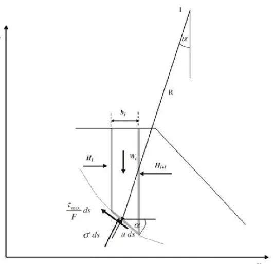
In the above, 𝐹𝑆 is the factor of safety, and banks are considered unstable when 𝐹𝑆 < 1, and for any slice 171
𝑖 (Fig. 1), 𝑊𝑖 is the weight; 𝑏𝑖 is the river width; 𝑢𝑖 is the pore water pressure at the bottom of the slice; 𝛼𝑖 172
is the angle between the vertical and the radius 𝑅 of the circular slip surface; 𝑐′
𝑖 is the effective cohesion 173
and ∅′
𝑖is the effective angle of friction. In Fig.1, 𝐻 refers to the horizontal interslice force, and 𝐼 represents 174
the center of a trial circle of radius 𝑅.Interested readers can refer to (Mahdi 2004; Mahdi and Merabtene 175
2010) for further details concerning the numerical implementation. 176
BISHOP combines the bank geometry and bank soil geotechnical properties (effective cohesion, 177
undrained cohesion, interior effective friction angle, and saturated unit weight) in the same input file. One 178
to nineteen stratigraphic layers might be defined for each riverbank, with each layer having its own 179
geotechnical properties as well as pore water pressure conditions. In addition, the model can be adjusted 180
when applied to a watercourse submerged by water; it takes into account the hydrostatic water pressure 181
by assuming the surface water as a soil layer of unit weight equal to that of water but with no shear 182
strength. 183
8
The BISHOP model was mainly used in the study instead of conventional software (i.e., GeoSlope, 184
SLOPE/W) to facilitate the automatic coupling of the models. In fact, the conventional software were 185
avoided since they require the model user to draw the bank profile and its different geotechnical layers as 186
well as the groundwater table, which is impractical in this study since many hydraulic cross-sections must 187
be analyzed during the flooding event which will be tedious and time consuming to do for each riverbank. 188
REDISSED Submodel 189
REDISSED is a sediment redistribution submodel developed by (Mahdi 2004) to reshape the bank 190
profiles following a circular failure. The model conserves the mass and accommodates the observed 191
failure form of the banks in the study site. In the case of bank failure, the model redistributes the bank-192
derived materials in the flow section where their erosion and/or transport will be determined by the 193
subsequent hydraulic conditions incorporated in the mobile-bed model. 194
As stated above, since there is no consensus among researchers regarding the redistribution of the 195
derived bank materials (Darby and Delbono 2002; Nagata et al. 2000; Pizzuto 1990), the authors 196
considered a field-based approach implemented in the REDISSED submodel. It consists of redistributing 197
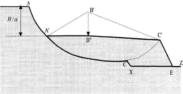
the failed materials as follows: The initial bank geometry is first described by a set of points (mesh nodes); 198
for simplification purposes, we consider the points ABCXZ plotted in Fig. . In the case of bank failure, the 199
circular sliding surface is along points ADC. The ABCD block is rotated so that the difference in altitude 200
between A and its image A’ will be equal to 𝐻 𝛼⁄ , where 𝐻 is the failure height (the difference in altitude 201
between points A and C) and 𝛼 is a coefficient greater than unity and is specified by the user based on 202
observations of the study site. Point B’, the image of B, is projected orthogonally to obtain point B’’ as 203
shown in Fig. . 204
Fig. illustrates the new bank profile defined by the points AA’B’’C’EZ, where point E belongs to section 205
XZ, so that A’B’C’B’’A’ and CC’EXC have equal areas for mass (or area) conservation purposes. 206
In a nutshell, the slump blocks undergo a rotation followed by a translation that moves the upper end of 207
the sliding bank to the bottom of the cross-section while conserving the mass. Once the submodel 208
redefines the form of the failed blocks, the topography of the bank section is automatically updated 209
accordingly before moving on to the next hydraulic time step. Meanwhile, the geotechnical layers are 210
9
updated through linear interpolation assumptions between the different points defining the geotechnical 211
layers. 212
Sliding cone area 213
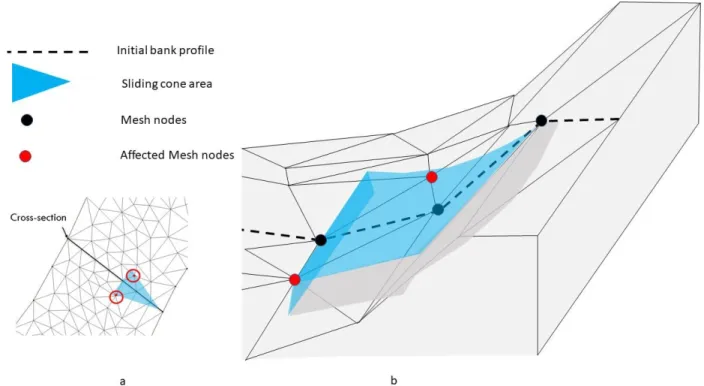
Redistribution of the mass wasting deposits of the unstable talus will be performed by using REDISSED 214
(Mahdi 2004) along the predefined cross-sections. However, the unstable failure block is a 2D planar 215
surface. Hence, to ensure the fully two-dimensional aspect of the study, the authors considered a sliding 216
bank area in the shape of a right cone with its axis as the cross-section line, its vertex as the upper point 217
of intersection between the riverbank and the slip circle computed by BISHOP (Mahdi 2004), and its 218
opening angle is a user-defined parameter (Fig. ). The mesh nodes located within the sliding cone area 219
will have their topography automatically interpolated to accommodate the new reshaped bank profile. The 220
mesh nodes affected by the failure will have a vertical displacement according to their position with 221
respect to the new bank geometry, i.e., 222
𝑍𝑀= 𝑍𝐵′′+ 𝑑𝑀
𝑑 × (𝑍𝐶′− 𝑍𝐵′′) (2) 223
where 𝑍𝑀 is the mesh node elevation obtained by interpolation; 𝑍𝐵′′ and 𝑍𝐶′ are the elevations of the 224
mesh nodes 𝐵′′ and 𝐶′, respectively, belonging to the new bank profile; 𝑑𝑀 is the distance from the node 225
𝐵′′, the nearest mesh node from node 𝑀; and 𝑑 is the distance between the two mesh nodes 𝐵′′ and 𝐶′. 226
The choice of the mesh nodes to be used for interpolation is done automatically, and the x coordinate of 227
the interpolated mesh node (𝑀) should be between the abscissa of the two mesh nodes, here nodes 𝐵′′ 228
and 𝐶′. 229
Coupling SRH-2D and BISHOP-REDISSED 230
The coupling between models started by incorporating bathymetric and topographic data on the SMS in 231
a similar fashion to the conventional mobile-bed and sediment transport modeling with SRH-2D, and 232
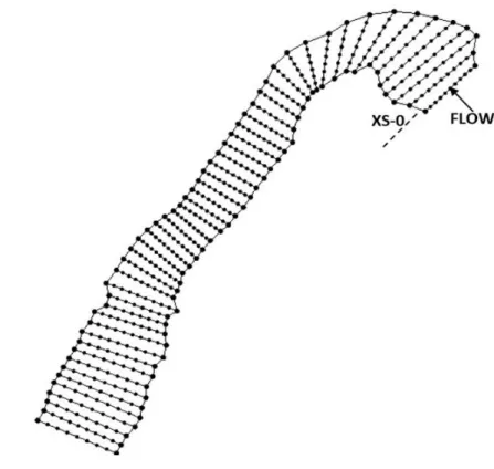
defining the cross-sections where the stability analysis will be performed. They will be set as node strings 233
on the SMS just before generating the mesh (Fig. ). Aftergenerating the mesh (Fig. ) and assigning the 234
10
boundary conditions, the pre-established cross-sections will be defined as monitor lines (maximum of 98 235
monitor lines) to get access to their nodes when exporting data. All other necessary modeling inputs 236
(Manning’s roughness, materials, simulation time, and initial conditions) can be fixed; thereafter, the key 237
simulation data can be exported to three principal files, the most important of which holds the node 238
coordinates at the monitor lines. This file will be used to ensure automatic feedback between the vertical 239
changes predicted by the 2D mobile-bed model and the lateral changes predicted by the geotechnical-240
stability and sediment-redistribution model BISHOP-REDISSED. 241
Assessing the geotechnical stability of the riverbanks and updating automatically the flow-wise 2D 242
geometry in case of bank failure for a long-reach-scale system without having to manually move the mesh 243
is seen as a key contribution of this study. Significant effort was expended to find a suitable procedure to 244
model hydraulic sections while considering their geotechnical characteristics. Herein, each cross-245
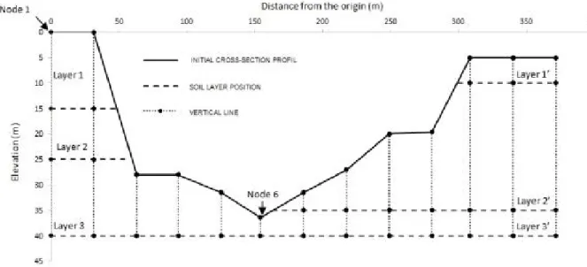
section was modeled as a set of vertical lines whose abscissa are the mesh nodes defining the transects. 246
These vertical lines form points of intersection at each change in the geotechnical properties of the 247
predefined layers (Fig. ). Thus, two text files are used in compiling geometric and geotechnical data. The 248
geometric file stores data in a vector whose components are the x-coordinate of the vertical line, the 249
elevation of the highest point of the cross-section and the elevation of the base of the different 250
geotechnical layers. We note that it is also possible to include the elevation of the crevice if it exists and 251
the elevation of the water level in it. Similarly, the geotechnical file regroups the geotechnical properties of 252
each soil layer for each riverbank profile separately, which includes the values of the effective cohesion 253
𝑐′, the undrained cohesion 𝑐
𝑢, the unit weight 𝛾′ and the interior effective friction angle ∅′ as well as the 254
elevation of the groundwater table or the pore pressure ratio 𝑟𝑢. It is worth mentioning that the global 255
coordinates of the nodes of the mesh in the SMS will be automatically transformed, translated and 256
rotated to have local coordinates with an origin at the far-left bank node of each cross-section (Node 1 in 257
Fig. ). These coordinates will be used to define the geometric files for BISHOP model. This is a 258
fundamental and necessary step since it will avoid distortion when updating the mesh and yet allows 259
consideration of river sinuosity. 260
11
Having defined the hydraulic and geotechnical parameters, the next step consists of launching the 261
developed automation algorithm. With a text-based interactive user interface, the user defines the case 262
name, the number of cross-sections, the slope of the potential sliding cone and finally the time step Δt’ to 263
test the stability of the banks (Fig. ). The developed algorithm, which uses, inter alia, an AutoHotkey 264
script, will automatically launch the srh-pre and inputted SMS-exported files. The preprocessor stage will 265
first check the possible errors and then output a directory file that contains the entire model input 266
information, especially the topography. That file will be used to launch the processor srh-2d automatically. 267
However, prior to that, the automation algorithm will make two principal modifications: 268
(1) The initial start time, time step and end time are among the simulation information stored on the 269
directory file. The initial simulation end time will be automatically changed to the BISHOP time 270
step Δt’. In addition, for the first run, the initial start time will be kept unchanged. However, starting 271
from the second run, the start time will be the end time of the previous simulation, and the new 272
end time will be Δt’ plus the start time. The simulation will accordingly last Δt’ of the flood event 273
for each run. The algorithm will call up the BISHOP model (Mahdi 2004) to evaluate the bank 274
stability at the end of each run. The program will launch SRH-2D several times (Nbtimes) and test 275
the bank stability at the end of each run until the total number of times is equal to the ratio 276
between the initial end time and the BISHOP time step Δt’ (Nbtotal). It is worth noting that the 277
chosen time step Δt’ should preferably be a divisor of the initial end time if not the hydraulic time 278
step. 279
(2) In addition to time information, the directory file records the name of the restart file, a file created 280
by the SRH-2D model in a previous simulation using the same mesh and hydraulic conditions. 281
The name of the file will be changed to the case name followed by _RST1. During each SRH-2D 282
simulation, the restart file is generated at each interval specified within the model control. Herein, 283
this file will be generated only at the end of each run and will be used as the initial condition of the 284
next simulation. This allows a continuation from the end of the previous simulation and thus takes 285
into account the last hydraulic-sediment transport conditions. 286
12
Following these few changes in the directory file, the program will launch the SRH-2D model for the first 287
run. The vertical model proceeds in its own time until it reaches the bank time step, when the BISHOP 288
model is activated. The SRH-2D model outputs a results file that describes the time-dependent evolution 289
of the cross-sections. The developed program will compare the node elevations of the cross-sections with 290
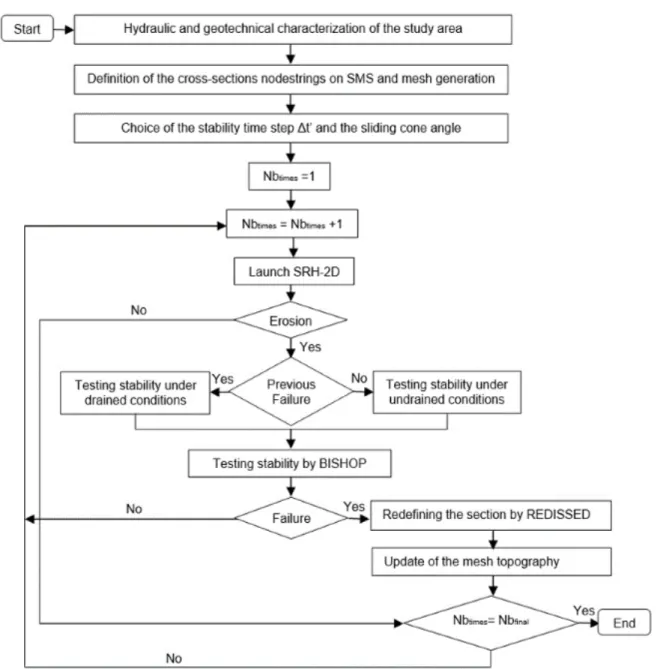
the initial elevation. In the absence of erosion, the analysis is advanced for the next time step, as 291
illustrated in the flowchart (Fig. ). If erosion occurs, at least around one riverbank, the new sections 292
representing the bed at the end of the time step are tested for the stability of their banks. The new cross-293
sections will be divided into two riverbanks from the lowest bed elevation (Node 6 in Fig. ). Each bank will 294
be subsequently coupled with its corresponding pre-established geotechnical properties files to define the 295
input files for BISHOP. Hence, the stability of the riverbank will be assessed; it will be performed under 296
drained conditions for the first potential bank failure and under undrained conditions afterwards. In fact, 297
after the first failure, the stability analysis will be performed using the resistance of the shear stress of the 298
undrained materials. This is due to the decrease in the interstitial pressure that allows the bank to resist 299
geometric changes over a certain timespan (Mahdi and Merabtene 2010) and then accounts for the 300
protection afforded by the failed materials. 301
In the absence of rupture (FS>1), the simulation is advanced for the next time step (Fig. ). Otherwise, the 302
bank profile will be reshaped based on the REDISSED (Mahdi 2004) submodel; the corresponding 303
geometric file will be updated to account for the new bank profile. Although the program will renew the 304
channel bed and bank topography based on the updated geometry, prior to that, the program will make 305
necessary transformations (translation and rotation) to adapt the new node coordinates to their initial 306
global system on the SMS. In addition, the bed topography of all the nodes located inside the sliding cone 307
area will be automatically interpolated to accommodate bank failure as illustrated in figure 9; the mesh will 308
therefore be updated before moving to the next hydraulic time step. 309
Once the bed topography is updated, the program will set the restart file as an initial condition to continue 310
from the last hydraulic-sediment transport conditions and ultimately make necessary changes in the start 311
and end times, as explained before. The simulation will run as many times as necessary until the initial 312
end time is achieved (see the application section below). 313
13
Application: case study
314
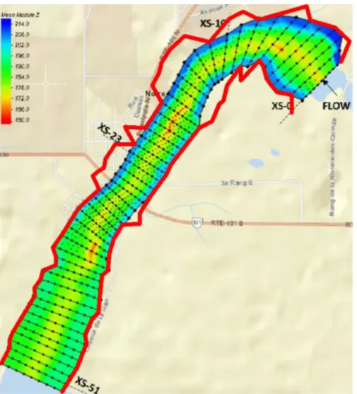
The approach adopted to verify the coupling procedure was applied over a long-reach scale; 7 kilometers 315
of river length extending from the Première Chute Dam to Lake Témiscamingue along the Outaouais 316
River at Notre-Dame-du-Nord, Quebec, was considered. The study reach is characterized by the 317
presence of cohesive sediments along the river, and the height of the local banks typically vary between 318
35 m high near the dam and 15 m high at the entrance of Lake Témiscamingue. It is an interesting field 319
site since the water never overflows, even in the case of dam failure; therefore, bank failures are the only 320
risk for the riverside population. 321
Model setup
322
A 2D mesh initial solution domain representing the initial channel topography of the study area was 323
prepared in the SMS. The solution domain includes the positions of the selected cross-sections, where 324
the geotechnical stability analysis will be performed, modeled as straight segments moving downstream 325
from right to left, where the 2D mesh node coordinates define the bank face geometry. Herein, 52 326
irregularly spaced cross-sections were selected (including inlet and outlet transects), as shown in Fig. . 327
The cross-sections were carefully chosen to consider the hydraulic features of the channel, they relatively 328
represent the field domain as they present the same soil characteristics and riverbank slopes around 329
them from field observations. 330
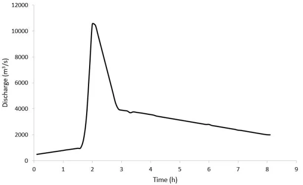
A time series discharge with a peak of approximately 9780 m3/s, which corresponds to the dam failure 331
scenario, was imposed upstream (Fig. ). A constant surface elevation of 179 m was enforced downstream 332
that corresponds to the water elevation in the lake. To represent the bed behavior, a constant Manning’s 333
roughness coefficient (𝑛) of 0.040 (𝑑50=160 mm) was used for the entire reach; it was estimated based 334
on field observations in 2002 (Thibault, 2002); no calibration was needed. The sediment transport 335
computation was carried out by using the Yang formula (Yang 1973), which is compatible with the bed 336
material of the reach, which was assumed to be made of the same material as the riverbanks. Note, 337
however, that the selection of the sediment transport equation is not important for the analysis below. 338
Table 1 lists the grain size composition of the bed and bank material segregated into seven size classes 339
14
supported by SRH-2D (Lai 2010). The volumetric compositions considering the seven classes listed in 340
Table 1 are 80%, 7%, 7%, 4%, 1%, 0% and 0%. 341
The geotechnical input parameters were prepared for each bank profile separately (104 bank profiles). 342
They consist of a single homogeneous cohesive layer with measured properties supplemented by field 343
test results carried out on some collected samples: effective cohesion 𝑐′=1.6 KPa; undrained cohesion 344
𝑐𝑢= 9 KPa; unit weight 𝛾′= 18.6 KN/m3; and interior effective friction angle ∅′=32°. The pore pressure 345
ratio, the ratio of the pore water pressure to the overburden pressure, was set to its maximum value 𝑟𝑢= 346
0.45 (Fredlund and Barbour 1986). In this regard, we emphasize that within BISHOP (Mahdi 2004; Mahdi 347
and Merabtene 2010), it is also possible to define pore water pressures given the pressure field or the 348
groundwater table. Since information was not available, we assumed the most unfavorable case and 349
chose the maximum pore pressure ratio. 350
The coupling procedure between SRH-2D (Lai 2010) and BISHOP (Mahdi 2004) was applied for 9 hours 351
of the event. The flow, sediment transport and bed evolution time step was set to 5 s, whereas the 352
stability analysis was carried out each Δt’ =0.125 h. The time scale to assess the geotechnical stability of 353
the banks is usually much greater than the time scales of hydrodynamic and channel bed morphological 354
evolution. A sensitivity analysis will be conducted later to explore the impact of the time scale on the 355
results of the model. Given the above values, the simulation will run 72 times (Nbtotal= 9/(Δt’)= 72), and at 356
the end of each run, the stability analysis will be assessed profile by profile. As stated earlier, to update 357
the flow-wise 2D geometry, a cone-shaped failure block was considered. Since there are no available 358
measured data regarding the extents of the failed area and because the mesh is relatively coarser, a 60° 359
opening cone angle was assumed in the case of bank failures. Finally, the REDISSED parameter 𝛼 was 360
set to 5.5 as suggested by (Thibault C et al. 2002) to represent the form of the failed banks at the study 361
site. 362
Results
363
Two different scenarios were simulated. The first scenario considered only vertical erosion modeling 364
using the SRH-2D (Lai 2010) model, and the second scenario combined vertical and lateral erosion 365
modeling using the coupling procedure. Error! Reference source not found. shows the initial and final 366
15
profiles for selected riverbanks considering both scenarios, Fig. 13 shows the bank retreat plan view and 367
Fig.14 shows a 3D view of a redefined bank profile. The evolution of the factor of safety for the riverbanks 368
during the simulation period is illustrated in Error! Reference source not found.. Furthermore, the 369
predicted net bank retreat distances for all the cross-sections are displayed in Fig. . 370
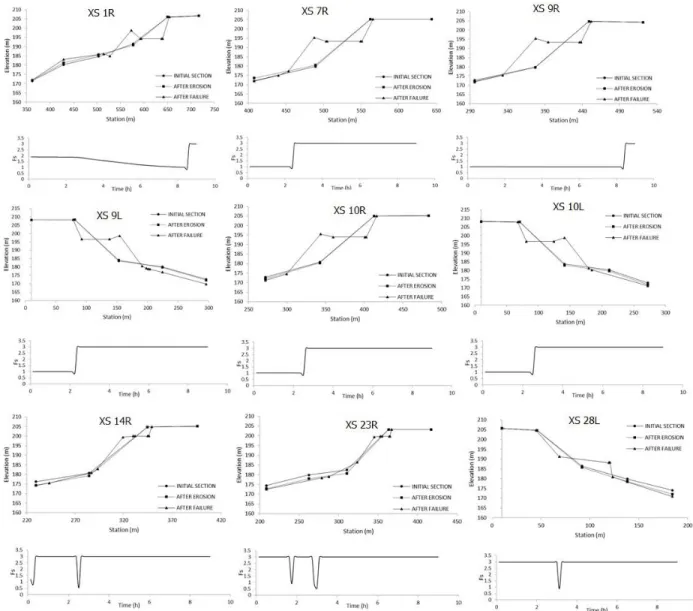
These results show that bank failures are mostly observed alongside the bend and in the upstream 371
section above it, where banks are high and steep. The bank retreat process was particularly significant 372
within the river bend, which reveals a bank retreat up to 6 m for cross-sections 13 to 16, particularly on 373
the right bank section (Fig. ). This can most likely be attributed to the optimal combination of slope and 374
flow, to similarities in bank geometry and to the relatively narrower cross-sections in that area. In fact, 375
fluvial erosion seems to have contributed more to steepening the bank profiles upstream, making them 376
susceptible to geotechnical failures. Downstream, bank failures were almost absent, flow velocity and 377
shear stress were smaller, bank heights and slopes were lower, and the channel morphological changes 378
were then exclusively dominated by fluvial erosion. 379
Moreover, the erosion of the channel bed is noticeably stronger when exhibiting the bank failure process, 380
especially for the first cross-sections (7R, 9L, and 9R) (hereafter denoting L for the left bank and R for the 381
right bank) and along the bend (10L,10R and 14R). The failed bank-deposited materials downslope seem 382
to serve as temporary protection from the fluvial erosion but make the cross-sections narrower and the 383
slopes steeper, which increase the speed of the flowing water and the channel bed erosion rate. 384
Furthermore, this rate appears to be related to the timing of the mass failure. In fact, the channel bed 385
zone of the transects where the banks were predicted to fail early have been eroded more (9L, 14R, 23R 386
and 28L) compared to those that failed later (1R and 9R) where the simulated bed deepening is 387
approximately the same when considering the fluvial erosion only. This may be justified because the bank 388
predicted to fail earlier becomes much more stable over the rest of the simulation period, which makes 389
the channel narrower for a long period. Indeed, after the first bank failure, we hypothesize that bank 390
stability will be evaluated with undrained conditions, which enhance the geotechnical stability of the bank. 391
In addition, as stated above, the protection afforded by the failed materials further increases their stability, 392
as the failed materials have to be removed first by fluvial erosion. Together, these findings explain the 393
16
slightly higher channel bed erosion rate for banks predicted to fail earlier compared to those that failed 394
later. 395
Furthermore, after the bank failure, we note that the bank geometry was reshaped, and the failed blocks 396
were redistributed along the cross-section. The redistribution of the eroded materials is clearly visible for 397
the banks that failed later (1R and 9R) since the fluvial erosion did not consume all the material deposits. 398
However, the volume of the failed bank materials is seen to be reduced for banks that failed earlier (14R, 399
23R). In addition, the slump blocks have been redistributed all around the neighboring transects 400
considering the failure cone shape assumption established in the process of this study. Fig. shows the 401
bank geometry profile of the cross-sections neighboring the failed bank at cross-section 10, where the 402
bed elevations of the mesh nodes were displaced to account for the newly defined bank profile. 403
Sensitivity to the BISHOP time step 404
Sensitivity analysis was completed to determine the impact of the geotechnical stability analysis time step 405
on the bank failure prediction and retreating distances. Simulations with different time steps were run 406
using 0.0625, 0.125, 0.25 and 0.5 h. The selected time steps are all divisors of the simulation total time (9 407
hours) to ensure having the necessary runs to reach it. Hence, the simulation was run 144, 72, 36 and 18 408
times for each time step. By doing so, we reasonably hypothesize that the closer the BISHOP (Mahdi 409
2004) time step is to the SRH-2D (Lai 2010) time step, the more we are certain to capture all the potential 410
riverbank failures. 411
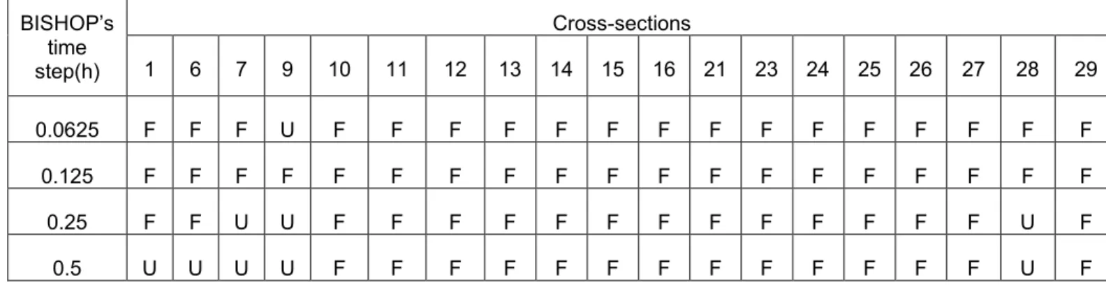
Fig. shows the retreating bank distances for the right and left top bank lines for different geotechnical 412
time steps. Table 2 lists only riverbanks that were predicted to fail for certain time steps but not for others. 413
As expected, more banks were predicted to fail while decreasing the BISHOP (Mahdi 2004) time step. In 414
fact, the right bank at cross-section 7 and the left bank at cross-section 28 were predicted to fail for both 415
time steps 0.0625 and 0.125 h but not for the highest time steps. Three and even four bank failures were 416
missed for time steps of 0.25 and 0.5 h; the flow conditions have perhaps changed, and the banks are no 417
longer unstable. However, we note that the left bank at cross-section 9 was predicted to fail when 418
considering time step 0.125 but not time step 0.0625. This can be attributed to the BISHOP (Mahdi 2004) 419
17
order of accuracy. Fig. shows that the factor of safety was very close to unity; to three decimal places, 420
the bank was considered, though, stable. 421
Moreover, the timing of bank failure seems to be accurately predicted using small time steps (0.0625 and 422
0.125). Fig. shows the evolution of the factor of safety at the left bank of cross-section 10 considering the 423
four configurations. The failure occurs 2.375 hours from the start of the simulation when using time steps 424
of 0.0625 and 0.125 h. However, the riverbank was predicted to fail later for the two other time steps 425
(almost one hour later). This can most likely be justified by the subsequent failures along the directly 426
neighboring transects of the channel bank. In fact, the left bank of transect 9 was predicted to fail 2 hours 427
after the simulation begins when using 0.0625 and 0.125 time steps but not for the highest time steps. 428
This probably impacted the 10L bank failure time when using 0.25- and 0.5 time steps, as the channel 429
bank form in that area was different. Although the 10L bank profile was slightly the same for the four 430
different time steps (not shown), the difference between the timings was insignificant compared to the 431
total remaining time of the simulation. 432
Overall, despite the timing issues highlighted above, we notice that the predicted bank retreat area and 433
the retreating bank distances were considerably close for the small time steps (Fig. ). The model was 434
nevertheless capable of capturing the potential troubling spots without regard to the chosen time step. We 435
recommend, however, using small time steps to improve predictions of the retreat location with respect to 436
the computational cost of the simulation. 437
Discussion
438
Despite the overall success in predicting the bank retreat and redistributing the removed unstable failure 439
blocks, some aspects of the study need more attention. First, the predicted bank retreat depends on the 440
mesh size considered. With the current mesh, the bank zone is badly represented, an average of ten 441
lateral nodes define the transects, which unsatisfactorily capture the bank face geometry and would yield 442
to a scarce bank retreating prediction. Second, after bank failure, only a few neighboring cross-sections 443
were reshaped to account for the newly defined bank profile, perhaps because of the cone interior angle 444
and again the mesh density. Indeed, we used a relatively coarser mesh, and few elements were affected. 445
The mesh was locally refined at cross-section 10 to take account of the newly reshaped bank profile as 446
18
illustrated in Fig. 20; further mesh refinement may allow defining the sliding area accurately but increases 447
the study computational cost and may induce model divergence, as the mesh representing the failed 448
banks might be distorted considerably. The cone interior angle considered could affect the extent of the 449
sliding area, especially for a much-refined mesh. The angle of 60° was set as an assumption in the 450
present study, a sensitivity analysis might be conducted to evaluate the influence of the angle but it is 451
outside the scope of this research. Third, after bank failure, the REDISSED (Mahdi 2004) submodel 452
reshapes the bank profile as described in detail earlier, although the submodel adds some supplementary 453
points to correctly represent the geometry of the bank face toward ensuring mass conservation. However, 454
the elevation of those additional points will be used to shift the mesh node elevations using a simple 455
linear interpolation method, which may induce loss of precision. Higher-order interpolation functions could 456
potentially yield better accuracy but were abandoned during the study since it would be reasonable and 457
suitable to combine the functions with a much finer mesh. Fourth, the fluvial erosion rate before and after 458
the bank failure was considered the same, which might be incorrect as the critical shear stress of the 459
materials differs, but this was also an assumption that we have made in the present research, which 460
seems to be acceptable since it does not affect the objectives of the study. Finally, the pore pressure ratio 461
was considered constant for all the banks, which might influence the bank failure prediction since 462
cohesive banks are more susceptible to failure during rapid-drawdown, high-flow events (Alonso and 463
Pinyol 2016). The constant pore pressure ratio was again an assumption that we considered in the 464
present study and might be a subarea for future improvement. 465
Streambank erosion modeling of the river reach extending from the Première Chute Dam to Lake 466
Témiscamingue along the Outaouais River was very challenging. The reach longitudinal length was 467
approximately 7 km, the banks are very tall and steep, and landslides along this river reach are the 468
predominant existing risk. Simulation of the river reach evolution was conducted considering a dam break 469
scenario that requires a frequent decrease in the hydraulic time step to ensure model convergence. 470
Notwithstanding those difficulties, up to 100 m of bank retreat was predicted at several riverbanks (Fig. ), 471
and almost 20 cross-sections were reshaped using the developed coupling procedure. Typical results 472
demonstrating the effectiveness of the developed methodology were presented in the study. Importantly, 473
the model allows the automatic prediction of bank retreat due to both fluvial erosion and geotechnical 474
19
failure in long-reach-scale modeling systems using a 2D mesh in a simple and easy-to-use manner. 475
Without survey data, the model is valid primarily for the identification of potential trouble spots for streams 476
without necessarily requiring various input parameters. 477
Conclusion
478
In this paper, a new platform coupling a 2D mobile-bed modeling software, SRH-2D, a rotational failure 479
analysis model, BISHOP, and a bank failure sediment-redistribution submodel, REDISSED, was 480
developed. The major contributions are the redistribution of the slump blocks produced by riverbank mass 481
failures onto the 2D mesh while conserving the mass; automation of the data exchanges between the 482
different models, which makes the simulation less tedious; and finally, the robustness and ease of use of 483
the model, which makes it applicable to practical stream events. 484
The developed coupling procedure has been applied to simulate the channel morphology of the 485
Outaouais River at Notre-Dame-Du Nord; considering the complexities of the study site and the shortage 486
of geotechnical and survey data, all four established objectives were nonetheless attained. The coupling 487
approach showed encouraging results; up to 100 m of bank retreat was predicted, and the bank faces of 488
over 20 cross-sections were renewed. However, the study can be further enhanced. In this field 489
application, it has been noted that redistribution of unstable blocks is done merely along the failed banks, 490
yet the bed elevations of only a few nodes of the neighboring cross-sections were updated. The study can 491
accordingly be improved by integrating a more accurate submodel capable of evaluating the extent of the 492
slumped area based on the real topography and soil properties, which could be an interesting area of 493
future research. Moreover, given the influence of pore pressure on the factor of safety (Casagli et al. 494
1999), it would be beneficial to improve the BISHOP model by coupling it to a hydrogeological model 495
giving the distribution of interstitial pressure in the soil instead of fixing a constant pore pressure ratio for 496
all the riverbanks during the simulation period. Finally, nonfluvial processes such as seepage or rainfall 497
events were not included in this study. Those processes could also impact the streambank erosion 498
predictions; the fluvial process-based models alone are insufficient. Modeling those nonfluvial processes 499
is another avenue for future research. 500
20
Acknowledgment
501
This research was supported in part by a National Science and Engineering Research Council (NSERC) 502
Grant and Hydro-Quebec. 503
Notation
504
The following symbols are used in this paper: 505
𝑏𝑖 Slice width 506
𝑐’ Effective cohesion 507
𝑐’𝑖 Effective cohesion of the slice 508
𝑐𝑢 Undrained cohesion 509
𝑑 Distance between two mesh nodes 510
𝑑50 Diameter at which 50% of a sample’s mass is comprised of smaller particles 511
𝐹𝑆 Factor of Safety 512
𝐻 The failure height 513
𝑖 Slice 514
𝐿 Left bank 515
𝑁𝑏𝑡𝑖𝑚𝑒𝑠 Number of times to launch SRH-2D 516
𝑁𝑏𝑡𝑜𝑡𝑎𝑙 The total number of times to launch SRH-2D 517
𝑅 Right bank 518
𝑟𝑢 Pore pressure ratio 519
𝑢𝑖 Pore pressure ratio at the bottom of the slice 520
21
𝑊𝑖 Slice Weight 521
𝑍 Mesh node elevation 522
𝛼 Coefficient greater than the unity, specified by the user based on field observation 523
𝛼𝑖 Angle between the vertical and the radius of the circular slipe surface 524
∅’ Interior effective friction angle 525
∅’𝑖 Interior effective friction angle of the slice 526
𝛾’ Saturated unit weight 527
∆𝑡’ Time step to test banks stability 528
References
529
Abad, J. D., and Garcia, M. H. (2006). "RVR Meander: A toolbox for re-meandering of channelized 530
streams." Computers & Geosciences, 32(1), 92-101. 531
Alonso, E. E., and Pinyol, N. M. (2016). "Numerical analysis of rapid drawdown: Applications in real 532
cases." Water Science and Engineering, 9(3), 175-182. 533
AQUAVEO (2019). "SMS 12.3 - The Complete Surface-water Solution.", 534
<http://www.aquaveo.com/software/sms-surface-water-modeling-system-introduction>. (June 10, 535
2019). 536
ASCE Task Committee on Hydraulics, B. M., and Modeling of River Width Adjustment (1998). "River 537
width adjustment II: Modeling." Journal of Hydraulic Engineering, 124(9), 903-917. 538
Casagli, N., Rinaldi, M., Gargini, A., and Curini, A. (1999). "Pore water pressure and streambank stability: 539
results from a monitoring site on the Sieve River, Italy." Earth Surface Processes and Landforms: 540
The Journal of the British Geomorphological Research Group, 24(12), 1095-1114.
541
Darby, S. E., and Delbono, I. (2002). "A model of equilibrium bed topography for meander bends with 542
erodible banks." Earth Surface Processes and Landforms: The Journal of the British 543
Geomorphological Research Group, 27(10), 1057-1085.
544
Darby, S. E., Rinaldi, M., and Dapporto, S. (2007). "Coupled simulations of fluvial erosion and mass 545
wasting for cohesive river banks." Journal of Geophysical Research: Earth Surface, 112(F3). 546
Fredlund, D. (1995). "User’s guide SLOPE/W." GEO-SLOPE International, Ltd., Calgary, Alb. 547
Fredlund, D., and Barbour, S. (1986). "The prediction of pore pressure for slope stability analysis." Proc., 548
Slope Stability Seminar, Univ. of Saskatchewan, Saskatoon, SK.
22
Galland, J.-C., Goutal, N., and Hervouet, J.-M. (1991). "TELEMAC: A new numerical model for solving 550
shallow water equations." Advances in Water Resources, 14(3), 138-148. 551
Highland, L., and Bobrowsky, P. T. (2008). The landslide handbook: a guide to understanding landslides, 552
US Geological Survey Reston. 553
Lai, Y. (2008). "SRH-2D version 2: Theory and User’s Manual, Sedimentation and River Hydraulics–Two-554
dimensional River Flow Modeling." US Department of the Interior, Bureau of Reclamation, 555
Technical Service Center, Denver, CO.
556
Lai, Y. (2017). "Modeling Stream Bank Erosion: Practical Stream Results and Future Needs." Water, 557
9(12), 950. 558
Lai, Y. G. (2010). "Two-dimensional depth-averaged flow modeling with an unstructured hybrid mesh." 559
Journal of Hydraulic Engineering, 136(1), 12-23.
560
Lai, Y. G., Greimann, B. P., and Wu, K. (2010). "Soft bedrock erosion modeling with a two-dimensional 561
depth-averaged model." Journal of Hydraulic Engineering, 137(8), 804-814. 562
Lai, Y. G., Smith, D. L., and Israel, J. (2016). "2D and 3D Flow Modeling of the Sacramento River 563
Fremont Weir Section." Proc., World Environmental and Water Resources Congress 421-432. 564
Lai, Y. G., Thomas, R. E., Ozeren, Y., Simon, A., Greimann, B. P., and Wu, K. (2012). "Coupling a two-565
dimensional model with a deterministic bank stability model." Proc., Proceedings of the ASCE 566
World Environmental and Water Resources Congress, Albuquerque, NM, USA, 1290-1300.
567
Lai, Y. G., Thomas, R. E., Ozeren, Y., Simon, A., Greimann, B. P., and Wu, K. (2015). "Modeling of 568
multilayer cohesive bank erosion with a coupled bank stability and mobile-bed model." 569
Geomorphology, 243, 116-129.
570
Langendoen, E. J. (2000). Concepts: Conservational channel evolution and pollutant transport system, 571
USDA-ARS Naitonal Sedimentation Laboratory. 572
Langendoen, E. J., Mendoza, A., Abad, J. D., Tassi, P., Wang, D., Ata, R., El kadi Abderrezzak, K., and 573
Hervouet, J.-M. (2016). "Improved numerical modeling of morphodynamics of rivers with steep 574
banks." Advances in water resources, 93, 4-14. 575
Langendoen, E. J., and Simon, A. (2008). "Modeling the evolution of incised streams. II: Streambank 576
erosion." Journal of hydraulic engineering, 134(7), 905-915. 577
Langendoen, E. J., Wells, R. R., Thomas, R. E., Simon, A., and Bingner, R. L. (2009). "Modeling the 578
evolution of incised streams. iii: model application." Journal of Hydraulic Engineering, 135(6), 579
476-486. 580
Lavoie, B., and Mahdi, T.-F. (2017). "Comparison of two-dimensional flood propagation models: SRH-2D 581
and Hydro_AS-2D." Natural Hazards, 86(3), 1207-1222. 582
Mahdi, T.-F. (2004). "Prévision par modélisation numérique de la zone de risque bordant un tronçon de 583
rivière subissant une rupture de barrage [Prediction by numerical modeling of the risk zone 584
bordering a section of river undergoing a dam break]."Ph.D. Thesis, Ecole Polytechnique de 585
Montréal, Quebec, Canada. 586
Mahdi, T.-F., and Merabtene, T. (2010). "Automated numerical analysis tool for assessing potential bank 587
failures during flooding." Natural hazards, 55(1), 3-14. 588
Mahdi, T., and Marche, C. (2003). "Prévision par modélisation numérique de la zone de risque bordant un 589
tronçon de rivière subissant une crue exceptionnelle [Prediction by numerical modeling of the risk 590
23
zone bordering a section of river undergoing an exceptional flood]." Canadian Journal of Civil 591
Engineering, 30(3), 568-579.
592
Moges, E. M. (2010). "Evaluation of sediment transport equations and parameter sensitivity analysis 593
using the SRH-2D Model." Universität Stuttgart. 594
Motta, D., Abad, J. D., Langendoen, E. J., and Garcia, M. H. (2012). "A simplified 2D model for meander 595
migration with physically-based bank evolution." Geomorphology, 163, 10-25. 596
Nagata, N., Hosoda, T., and Muramoto, Y. (2000). "Numerical analysis of river channel processes with 597
bank erosion." Journal of Hydraulic Engineering, 126(4), 243-252. 598
Philiponnat, G., and Hubert, B. (1979). "Fondation et ouvrage en terre." Eyrolles, 19-20. 599
Pizzuto, J. E. (1990). "Numerical simulation of gravel river widening." Water Resources Research, 26(9), 600
1971-1980. 601
Rinaldi, M., Mengoni, B., Luppi, L., Darby, S. E., and Mosselman, E. (2008). "Numerical simulation of 602
hydrodynamics and bank erosion in a river bend." Water Resources Research, 44(9). 603
Rousseau, Y. Y., Van de Wiel, M. J., and Biron, P. M. (2017). "Simulating bank erosion over an extended 604
natural sinuous river reach using a universal slope stability algorithm coupled with a 605
morphodynamic model." Geomorphology, 295, 690-704. 606
Simon, A., Curini, A., Darby, S. E., and Langendoen, E. J. (2000). "Bank and near-bank processes in an 607
incised channel." Geomorphology, 35(3-4), 193-217. 608
Simon, A., Doyle, M., Kondolf, M., Shields Jr, F., Rhoads, B., and McPhillips, M. (2007). "Critical 609
Evaluation of How the Rosgen Classification and Associated “Natural Channel Design” Methods 610
Fail to Integrate and Quantify Fluvial Processes and Channel Response 1." JAWRA Journal of 611
the American Water Resources Association, 43(5), 1117-1131.
612
Simon, A., Pollen-Bankhead, N., and Thomas, R. E. (2011). "Development and application of a 613
deterministic bank stability and toe erosion model for stream restoration." Stream restoration in 614
dynamic fluvial systems, 453-474.
615
Thibault C, Leroueil S, and J, L. (2002). "Évolution des berges de rivière en cas de rupture de barrage: 616
cas du barrage Première-Chute." Université Laval, Québec. 617
Thorne, C. (1982). "Processes and mechanisms of river bank erosion." Gravel-bed rivers, 227-271. 618
Yang, C. T. (1973). "Incipient motion and sediment transport." Journal of the hydraulics division, 99(10), 619
1679-1704. 620
Yang, C. T. (1976). "Minimum unit stream power and fluvial hydraulics." Journal of the hydraulics division, 621
102(7), 919-934. 622
Yang, C. T., Trevino, M. A., and Simoes, F. J. (1998). User's Manual for GSTARS 2.0 (Generalized 623
Stream Tube Model for Alluvial River Simulation Version 2.0), US Department of Interior, Bureau
624
of Reclamation. 625
626 627
24
Figures Captions
628
Fig. 1. Equilibrium of a soil layer (simplified Bishop method) (Mahdi 2004)). 629
Fig. 2.Initial geometry and circular failure (Scale-adjusted to display the details)((Mahdi 2004)). 630
Fig. 3.Redistribution of the slump blocks following a circular failure (Scale-adjusted to display the details) 631
((Mahdi 2004)). 632
Fig. 4. Top view of the extents of the failed area defined within a cone-shaped form. The elevation of 633
mesh nodes located in that area will be updated to account for the newly defined bank profile. 634
Fig. 5. The cross-sections before generating the mesh on the SMS. 635
Fig. 6. The cross-sections after generating the mesh on the SMS. 636
Fig. 7. The initial cross-section bed profile and the associated soil layers. 637
Fig. 8.The coupling procedure methodology. 638
Fig. 9. Sliding cone area and affected mesh nodes a) Plan view b) 3D view. 639
Fig. 10. The initial bathymetry for the Outaouais River at Notre-Dame-du-Nord, Quebec. 640
Fig. 11. The flood hydrograph at the upstream. 641
Fig. 12. The initial and final bank profiles for selected right and left riverbanks, and evolution of the factor 642
of safety during the simulation period 643
Fig. 13. The predicted bankline changes after dam break occurrence (Red line) (retreats are 10 times 644
exaggerated). 645
Fig. 14. The 3D view of a redefined bank profile. 646
Fig. 2. The predicted net bank retreat distances for all the predefined cross-sections. 647
Fig. 3. The left and right bank profiles for cross-sections upstream and downstream cross-section 10. 648
25
Fig. 17. The net bank retreat sensitivity to the BISHOP time step for the right and the left riverbanks. 649
Fig. 18. The evolution of the factor of safety of the right bank at cross-section 9. 650
Fig. 19. The evolution of the factor of safety of the right bank at cross-section 10 considering four different 651
geotechnical time steps. 652
Fig. 20. Sliding cone area and affected mesh nodes before and after refining the mesh for cross section 653
10. 654 655
26
Tables Captions
656
Table 1. Size ranges of seven sediment size classes used for the channel bed modeling. 657
Table 2. Riverbanks predicted to fail for different geotechnical time steps. 658
659 660 661
Table 3. Size ranges of seven sediment size classes used for the channel bed modeling 662
Sediment Size Class Size Range (mm)
1 0.0025 to 0.0625 2 0.0625 to 0.125 3 0.125 to 0.25 4 0.25 to 0.5 5 0.5 to 1 6 1 to 2 7 >2 663 664
Table 2. Riverbanks predicted to fail for different geotechnical time steps. F: Failed banks; U: Unfailed banks. 665 BISHOP’s time step(h) Cross-sections 1 6 7 9 10 11 12 13 14 15 16 21 23 24 25 26 27 28 29 0.0625 F F F U F F F F F F F F F F F F F F F 0.125 F F F F F F F F F F F F F F F F F F F 0.25 F F U U F F F F F F F F F F F F F U F 0.5 U U U U F F F F F F F F F F F F F U F 666 667
27 668
Fig. 4. Equilibrium of a soil layer (simplified Bishop method) (Mahdi 2004)). 669
670
Fig. 2.Initial geometry and circular failure (Scale-adjusted to display the details)((Mahdi 2004)). 671
28 672
Fig. 3. Redistribution of the slump blocks following a circular failure (Scale-adjusted to display the details) 673
((Mahdi 2004)). 674
675
Fig. 4. Top view of the extents of the failed area defined within a cone-shaped form. The elevation of 676
mesh nodes located in that area will be updated to account for the newly defined bank profile. 677
29 678
679
Fig. 5. The cross-sections before generating the mesh on the SMS. 680
681
Fig. 6. The cross-sections after generating the mesh on the SMS. 682
30 683
Fig. 7. The initial cross-section bed profile and the associated soil layers. 684
31 685
Fig. 8.The coupling procedure methodology. 686
32 687
Fig. 9. Sliding cone area and affected mesh nodes a) Plan view b) 3D view. 688
689
Fig. 10. The initial bathymetry for the Outaouais River at Notre-Dame-du-Nord, Quebec. 690
33 691
Fig. 11. The flood hydrograph at the upstream. 692
34 693
Fig. 12. The initial and final bank profiles for selected right and left riverbanks, and evolution of the factor 694
of safety during the simulation period 695
35 696
Fig. 13. The predicted bankline changes after dam break occurrence (Red line) (retreats are 10 times 697
exaggerated). 698
699
Fig. 14. The 3D view of a redefined bank profile. 700
36 701
Fig. 5. The predicted net bank retreat distances for all the predefined cross-sections. 702