HAL Id: hal-00984294
https://hal.archives-ouvertes.fr/hal-00984294
Submitted on 28 Apr 2014
HAL is a multi-disciplinary open access
archive for the deposit and dissemination of
sci-entific research documents, whether they are
pub-lished or not. The documents may come from
teaching and research institutions in France or
abroad, or from public or private research centers.
L’archive ouverte pluridisciplinaire HAL, est
destinée au dépôt et à la diffusion de documents
scientifiques de niveau recherche, publiés ou non,
émanant des établissements d’enseignement et de
recherche français ou étrangers, des laboratoires
publics ou privés.
interactive system
Noureddine-Yassine Nair-Benrekia, Pascale Kuntz, Frank Meyer
To cite this version:
Noureddine-Yassine Nair-Benrekia, Pascale Kuntz, Frank Meyer. Selecting a multi-label classification
method for an interactive system. Studies in Classification, Data Analysis, and Knowledge
Organi-zation, 2014, Data Analysis, Learning by Latent Structures, and Knowledge Discovery, pp.157-167.
�hal-00984294�
Selecting a multi-label classification method for
an interactive system
N.Y. Nair Benrekia1,2, P. Kuntz2
, and F. Meyer1
1
Orange Labs, AV. Pierre Marzin 22307 Lannion cedex France (yacinenoureddine.nairbenrekia, franck.meyer)@orange.com
2
LINA, la Chantrerie-BP 50609, 44360 NANTES cedex France [email protected]
Abstract Interactive classification-based systems engage users to coach learning algorithms to take into account their own individual preferences. However most of the recent interactive systems limit the users to a single-label classification, which may be not expressive enough in some organization tasks such as film classification, where a multi-label scheme is required. The objective of this paper is to compare the behaviors of 12 multi-label classification methods in an interactive framework where “good” predictions must be produced in a very short time from a very small set of multi-label training examples. Experimentations highlight important perfor-mance differences for 4 complementary evaluation measures (Log-Loss, Ranking-Loss, Learning and Prediction Times). The best results are obtained for Multi-label kNearest Neighbours (ML-kNN), Ensemble of Classifier Chains (ECC) and Ensem-ble of Binary Relevance (EBR).
1 Introduction
The usual classification systems do not allow users to directly interact with the learning models. Consequently, in practice, their results may deviate from their preferences. Modeling human preferences remains a difficult task, espe-cially for personalized systems where classical interviews are out of reach and large-scale behavioral logs are not available. An alternative is to embed the user into the learning process via an interactive visual support (Ware et al. (2000)). The user plays the role of a trainer for an automatic classification algorithm and steers it towards his/her desired concepts. More precisely, in a dynamical process, he/she can define a set of subjective labels Lton a set of
training examples Tt described by a set of features F and correct, if and/or
when necessary, the labels predicted by an automatic classifier on a set of unlabeled examples St.
Such interactive machine learning process has recently received increas-ing attention and found applications in several domains. For instance, for document organization, iCluster (Drucker et al. (2011)) is an interactive,
mono-label system that assists users with item-to-group and group-to-item recommendations. It only requires few user-classified examples. With a sim-ilar objective, Smart selection (Ritter and Basu (2009)) interactively helps users achieve complex file selections. Based on the restricted set of files se-lected by the user, it automatically generalizes the selection to the rest of the files. For social recommendation, ReGroup (Amershi et al. (2012)) assists users in the creation of personalized groups in social networks on the basis of a small list of friends provided by the user.
However, most of these interactive systems limit the user to a single-label classification which may not be sufficiently meaningful in some organization tasks where examples may belong to different labels. Interactive multi-label classification is the generalization of the interactive single-label classification where examples can be associated with more than one subjective label (L > 1). As an illustration, let us consider a very simplified example (Table 1) from the applicative context of Video-on-Demand (VoD) in which we are notably interested. We suppose that, after a short interaction t, a user has created a set Lt= {Funny, I like, Good music, Sad} of four preferred labels and associated
a set Tt= {Twilight, Ice age, Titanic, Kill Bill} of four films described by a
set of features F = {Year, Actor1, . . . } with their most relevant labels in Lt.
For instance, Titanic ∈ Ttis associated with the following three labels: I like,
Good music and Sad. The learning model suggests personalized predictions for selected unlabeled examples (e.g Sparkle ∈ Stand Man of Steel ∈ St) to
him (the user).
Table 1. Motivating example
Film Year Actor1 . . . Funny I like Good music Sad
Twilight 2008 R. Pattinson . . . 0 1 1 0 Ice age 2002 R. Romano . . . 1 1 0 0 Titanic 1997 L. DiCaprio . . . 0 1 1 1 Kill Bill 2003 U. Thurman . . . 1 1 0 0 Sparkle 2013 J. Sparks . . . ? ? ? ? Man of Steel 2013 H. Cavill . . . ? ? ? ?
Motivated by the growing number of recent interactive systems, our re-search intends to develop an interactive multi-label classification-based sys-tem for film recommendation in a VoD application. Its efficiency depends on the quality of the classifier, the visual restitutions and the interaction modal-ities. Its evaluation is consequently a difficult open question which requires competencies from different scientific communities.
In this paper, we restrict ourselves to the learning component: which are the classifiers that simultaneously withstand the interactivity and the multi-label related constraints? We here propose an experimental comparison of 12 multi-label classification methods adapted to interaction. Tests have been made on 5 classical benchmarks of increasing difficulties. We evaluate the predictive quality with two multi-label measures from the literature
(Log-Selecting a multi-label classification method for an interactive system 3
Loss and Ranking-Loss), and the efficiency is roughly assessed by the learning and prediction times. Our results highlight a variety of behaviors, and help us better understand the evolution of the performances while the training set grows. Let us note that, in this paper, we restrict ourselves to learning concepts of each individual or each family independently and we do not consider the collaborative multi-users framework as in the Smart Selection system (Ritter and Basu (2009)).
This paper is organized as follows. Section 2 precisely defines the objec-tives. Section 3 briefly recalls the main principles of the 12 multi-label clas-sifiers selected for the comparison. The benchmarks and the experimental protocol are described in Section 4. Finally, the obtained results are discussed in Section 5.
2 Problem statement
Throughout the paper, we consider a F-dimensional feature space F = {f1, . . . , fj, . . . , f|F |} such that dom(fj) ∈ R, and a L-dimensional label space
L = {λ1, . . . , λk, . . . , λ|L|} such that dom(λk) ∈ {0, 1} (0: irrelevant, 1:
rele-vant). Let D = {(xi, yi) | i = 1..|D|} be a multi-label dataset of |D| multi-label
examples. Each example xi= (x1i, . . . , x j i, . . . , x
|F |
i ) is associated with a set of
labels yi= (y 1
i, . . . , yik, . . . , y |L|
i ) with dom(xi) ∈ R|F |, dom(yi) ∈ {0, 1}|L|and
|yi| ≤ |L| where |yi| and |yi| are respectively the number of relevant and
irrel-evant labels of xi. A multi-label classifier h aims at producing labels of
unla-beled examples xi∈ S from a very small training set T ⊂ D, where S is a large
set case s.t. |T | << |S|. More precisely, ˆyi = h(xi) = (ˆyi1, . . . ,yˆik, . . . ,yˆ |L| i )
with dom( ˆyi) ∈ [0..1]|L|).
Madjarov et al. (2012) recently proposed an extensive experimental com-parison of methods for multi-label learning. Their study aimed at evaluating the predictive performances alongside the efficiency of 12 well-known multi-label classifiers with 16 evaluation measures. This thorough comparison led to the recommendation of RF-PCT, HOMER, BR and CC for multi-label classi-fication. Here, we add the interactivity constraints to the multi-label learning problem. Thus, an efficient classifier should be able to produce “good” predic-tions from a very small set of multi-label training examples, in a very short time. In the following, we consider three criteria which appeared to be the most important for the problem we are facing in the VoD framework:
1. Preservation of the label ordering. The user is more likely to be interested in a label-ranking than in a label-classification which hides the prediction confidence of each label,
2. Maximization of the similarity between the predicted scores and the ground-truth labels. Each label-prediction must be as close as possible to the true label,
3. Minimization of learning and prediction times. Time is an in-escapable factor in our interactive framework.
For the first two criteria, we have selected extensions of two classical mea-sures (ranking-loss and log-loss) for the multi-label case. The label ordering preservation is evaluated by the classical Ranking-Loss (RL) (Schapire and Singer (2000)) which indicates the number of times that irrelevant labels are ranked higher than relevant labels. More precisely, let us consider a ranking function ri that sorts the labels of each example xi with respect to their
pre-diction precision. We suppose that riis an increasing function with the quality
of the prediction: the highest rank (i.e., ri= |L|) is given to the most relevant
label and conversely (i.e., ri= 1). The Ranking-Loss function RL(h, S) of the
classifier h on the test set S is defined by
RL(h, S) = 1 |S| |S| ∑ i=1 1 |yi| × |yi| |(λa, λb) ∈ yi× yi: ri(ˆyia) < ri(ˆybi)|
It is defined on [0..1] and, as a loss measure, the lowest values indicate the best performances.
The ability of maximizing the similarity between the predicted scores and the ground-truth labels is measured by the Log-Loss measure (LL) (Read et al. (2009)): LL(h, S) = 1 |S| × |L| |S| ∑ i=1 |L| ∑ j=1 min(−(ln(ˆyij)×y j i+ln(1− ˆy j i)×(1−y j i)), ln(|S|))
It is defined on [0..ln|S|] and the lowest values are associated with good performances. Its upper artificial bound (i.e., ln|S|) limits magnitudes of the penalty. The LL measure provides large margins of contrasts between com-peting multi-label methods: worse label-errors are more harshly penalized.
For the classifier speed evaluation, we only consider the learning and pre-diction times (in seconds) independently. We are aware that they are closely linked to the implementation of the classifiers, and more accurate measures will be proposed in the next future. However, as all the algorithms have been implemented in the same framework, they provide first interesting tendencies of the complexity.
3 Multi-label methods
The multi-label learning approaches can be organized in three main families: 1. the problem transformation methods transform the multi-label learn-ing problem into one or several slearn-ingle-label classification or regression problems,
Selecting a multi-label classification method for an interactive system 5
2. the algorithm adaptation methods extend single-label learning algo-rithms for the multi-label data,
3. the ensemble methods use ensembles of classifiers either from the prob-lem transformation or the algorithm adaptation approaches.
Our numerical comparisons are based on 12 frequently used multi-label classifiers whose implementation is available on MEKA3
or MULAN4
multi-label learning libraries. These classifiers are listed below. Default parameters were always used except for ML-kNN: due to the small training subsets, the number of neighbours k was set to 1.
3.1 Problem transformation methods
We consider 5 problem transformation methods. (1) The Most Frequent label set is our Baseline. For a new instance, it returns the most frequent label set in the training set. (2) Binary Relevance (BR) is probably the most popu-lar transformation method. It learns |L| binary classifiers, one for each label (Schapire and Singer (2000)). (3) Classifier Chain (CC) is an extension of BR that not only trains one classifier per label but also extends the dimension-ality of each classifier’s training data with labels of the previous classifiers, in a chain, as new features (Read et al. (2009)). (4) Label Powerset (LP ) considers each unique label set in the training data as one of the classes of a multi-class classification task (Tsoumakas and Katakis. (2007)). And, (5) Calibrated Label Ranking (CLR) extends the Ranking by Pairwise Compar-ison (RPC) (H¨ullermeier et al. (2008)) by introducing an additional virtual label to separate the relevant labels from the irrelevant ones (F¨urnkranz et al. (2008)). Let us note that, for the problem transformation methods, two base-learners are commonly used (Madjarov et al. (2012), Read (2010)): Support Vector Machine (SVM) (Hearst et al. (1998)) and C4.5 decision tree (Quinlan et al. (1993)). We here preferred C4.5 decision tree for its low computational complexity: unlike SVM, it only requires a selected number of features for constructing a model. This choice is very important in our interactive learn-ing framework and even more when classifiers are trained on sets with a large number of features (e.g. our VoD data).
3.2 Algorithm adaptation methods
We consider 2 adaptation methods. (1) AdaBoost.MH is an extension of the famous AdaBoost which was implemented into the BoosTexter classification system for multi-label data (Schapire and Singer (2000)). It was designed to minimize the Hamming loss. (2) ML-kNN is a binary relevance method which extends the lazy learning algorithm kNN by using a Bayesian approach (Zhang et Zhou. (2007)). It retrieves the k nearest examples of each new instance, and then determines its label set from the maximum a posteriori principle (MAP).
3
http://meka.sourceforge.net/
4
3.3 Ensemble methods
We consider 3 ensemble methods. (1) The RAndom k labEL sets (RAkEL) constructs an ensemble of m LP classifiers. Each LP classifier is trained with a different random subset of a small size k (Tsoumakas and Vlahavas (2010)), (2) Hierarchy Of Multi-label classifiERs (HOMER) constructs a hierarchy of LP classifiers such that each classifier deals with a much smaller label set compared to L (Tsoumakas et al. (2008)). (3) Ensemble of Classifier Chains (ECC) and Ensemble of Binary Relevance (EBR) are ensemble methods whose base learners are CC and BR respectively (Read et al. (2009)).
4 Experimental setting
For the experimental comparison, we used 5 open datasets of various complex-ities (Table 2). These datasets are very small compared to the huge feature space of a VoD catalogue. Yet, they can provide first insights of the behav-ior properties of our selected classifiers. Emotions is a small dataset where each piece of music can be labeled with 6 emotions (e.g. sad-lonely, angry-aggressive, amazed-surprised). Yeast is a widely used biological dataset where genes can be associated with 14 biological functions. Scene is a dataset where images can be annotated with up to 6 concepts (e.g. Beach, Sunset, Moun-tain). Slashdot is a dataset where documents can be associated with 22 subject categories (e.g. linux, technology, science). And, a sample of IMDB dataset where movies can be labeled with 17 genres (e.g. Romance, Comedy, Drama). In order to evaluate both the predictive performance and the efficiency of each classifier, we have designed a simple experimental protocol that simulates a user that progressively classifies examples and that expects good predictions as a reward for his effort. The classifiers are tested on relatively large test sets using very small nested training sets (from 2 until 64 examples). The objective is to highlight the classifiers able to learn from restricted training sets in a short time and to measure their prediction improvement when the training sets double in size. Precisely, the experimental protocol is the following :
1. Divide each dataset D into 5 distinct folds. Use one fold for training (T = 20% of D) and the 4 remaining folds for test (S = 80% of D), and carry out a 5 cross-validation.
2. From each training set T , extract m sets of p nested training subsets of size 21
, 22
, . . . , 2p.
3. For each measure, evaluate the average performance of each classifier on the 5 test sets of each dataset. Each classifier is trained with the nested subsets of increasing size (21
, then 22
, . . . ; until 2p). Then, for each
classi-fier, compute the average performance on the 5 datasets for each training subset.
Selecting a multi-label classification method for an interactive system 7
For all experiments, m was fixed to 20 (100 tested sets for 5 cross-validations) and p to 64. The number of tested sets (m = 50) is sufficient to evaluate the global performance of each classifier. Larger values of m did not significantly improve the results. And, the threshold (p = 64) is consistent with real-life experiments where users do not annotate more than 64 examples by themselves without any assistance of a learning algorithm.
Table 2.Basic statistics of the selected multi-label benchmarks with DL: number of distinct label sets in each dataset, Lcard : average number of labels associated with examples in each dataset, n: numeric and b: binary
Dataset |F | |D| |T | |S| |L| #DL #Lcard Emotions 72n 592 118 474 6 27 1.87 Yeast 103n 2417 483 1934 14 198 4.24 Scene 294n 2407 481 1926 6 15 1.07 Slashdot 1079b 3782 756 3026 22 156 1.18 Imdb 1001b 7500 1500 6000 28 1021 2.00
5 Results
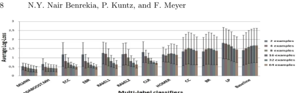
Let us note that the presented results are averages on all datasets, and that the differences between the datasets are evaluated by the standard deviations. In Figures 1 to 4, the classifiers are ordered according to their overall performance when considering together their average performances obtained per training subset size (from 2 to 64 examples).
5.1 Log-Loss
The Log-Loss measure intensifies the discrimination between competing meth-ods. Figure 1 clearly shows that the Multi-label k Nearest Neighbours (ML-kNN) and AdaBoost.MH outperform the other approaches with a slight ad-vantage for ML-kNN. ML-kNN, Ensemble of BR (EBR) and Ensemble of Classifier Chains (ECC) are known to get good performances for this measure (Read (2010)) whereas, to the best of our knowledge, AdaBoost.MH has not been yet evaluated with this later. Furthermore, the worst results are obtained for Label Power-set (LP), Binary Relevance (BR), Classifier Chain (CC) and our Baseline (the most frequent label-set). The following couples of methods share similar performances: (BR, CC), (EBR, ECC) and (Random k labEL-set 1 & 2). This is not surprising because CC is closely related to BR and (RAkEL1, RAkEL2) are variations of the original method RAkEL. However,
when the cardinality of the training subsets increases, only 8 algorithms are able to significantly improve their predictions. This is especially true for EBR and ECC.
Figure 1. Performances of the multi-label classifiers in terms of Log-Loss measure. Classifiers are ordered from left to right according to their average performances.
5.2 Rank-Loss
Roughly speaking, the orderings of the classifiers with the Log-Loss and the Rank-Loss measures are quite similar (Figure 2). This was expected since these measures are intuitively correlated. Nevertheless, a different behavior is ob-served for CLR and AdaboostMH; CLR is the best approach for the rank-loss and AdaBoost.MH moves from the 2nd place to the 6th. It is not surprising
to obtain the best results with CLR because it was specially designed to im-prove the quality of the predicted ranking (F¨urnkranz et al. (2008)). Similarly, ML-kNN aims at minimizing this measure. And, the ensemble methods pre-serve their ranks. The worst classifiers remain the same as with the Log-Loss measure. Moreover, when the training subset cardinalities increase CLR and ML-kNN are the fastest to improve the quality of the predicted ranking.
Figure 2.Performances of the multi-label classifiers in terms of Rank-Loss measure. Classifiers are ordered from left to right according to their average performances.
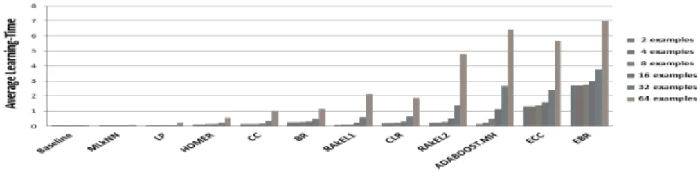
5.3 Computation time
As all our experiments were conducted with implementations of MEKA and MULAN libraries that are not necessarily optimized, the observed learn-ing/prediction times only provide a tendency of the algorithmic complexity (Figures 3 and 4). For instance, EBR is expected to be computationally faster than ECC but our results show the opposite. Among the three best classi-fiers (ML-kNN, ECC, EBR) for the previous measures, ML-kNN seems the fastest. It does not learn a model but it requires some milliseconds for the estimation of the prior and posterior probabilities from the training subset. And, it requires less than a 1
Selecting a multi-label classification method for an interactive system 9
neighbours is here small (k = 1). EBR and ECC seem to be more expensive but they are fast enough to finish learning and predicting within the first few seconds.
Figure 3. Performances of the multi-label classifiers in terms of Learning-Time. Classifiers are ordered from left to right according to their average performances.
Figure 4. Performances of the multi-label classifiers in terms of Prediction-Time. Classifiers are ordered from left to right according to their average performances.
6 Conclusion and future works
This paper studies the behaviors of different multi-label strategies in an inter-active setting where training data and computation time are limited resources. The final objective, whose description goes beyond this communication, is no-tably the development of an interactive classification system for film recom-mendation in a VoD application. Our comparison of 12 multi-label methods from the three main popular families (problem transformation, adaptations and ensemble methods) on 5 benchmarks of various complexities have shown that the best performances are reached by Multi-label k Nearest neighbours (ML-kNN), Ensemble of Classifier Chains (ECC) and Ensemble of Binary Relevance (EBR). However, the limitations of ML-kNN are well-known: its scaling is not assured because, in addition to a training stage, |T | operations are needed to predict labels of one instance only. That is quite expensive in both time and memory space. In addition, a metric learning stage may be required to bring out relevant features from the pool of irrelevant features. In spite of its limitations, ML-kNN is more efficient than ECC for larger training sets (Madjarov et al. (2012)). Since implementations of ECC and EBR are closely related, ML-kNN is here considered as the ”best” classifier for both small and large training data.
In the near future, we plan to extend the experiments to analyze the behavior of the classifiers on very large datasets where the number of features is very large (|F > 5000|) (e.g. our VoD data). Furthermore, we are willing to check whether the experimental learning and prediction times are consistent with the theoretical complexity.
References
Amershi, S., Fogarty, J., & Weld, D. (2012): Regroup: Interactive machine learning for on-demand group creation in social networks. In Proc. of the SIGCHI Conf.
on Human Factors in Computing Systems (pp. 21-30). ACM.
Drucker, S. M., Fisher, D., & Basu, S. (2011): Helping users sort faster with adaptive machine learning recommendations. In Human-Computer
Interac-tion–INTERACT (pp. 187-203). Springer Berlin Heidelberg.
F¨urnkranz, J., H¨ullermeier, E., Menc´ıa, E. L., & Brinker, K. (2008): Multilabel classification via calibrated label ranking. Machine Learning, 73(2), 133-153. Hearst, M. A., Dumais, S. T., Osman, E., Platt, J., & Scholkopf, B. (1998). Support
vector machines. Intelligent Systems and their Applications, IEEE, 13(4),
18-28.
H¨ullermeier, E., F¨urnkranz, J., Cheng, W., & Brinker, K. (2008): Label ranking by learning pairwise preferences. Artificial Intelligence, 172(16), 1897-1916. Madjarov, G., Kocev, D., Gjorgjevikj, D., & Dˇzeroski, S. (2012): An extensive
exper-imental comparison of methods for multi-label learning. Pattern Recognition,
45(9), 3084-3104.
Quinlan, J. R. (1993). C4. 5: programs for machine learning. Morgan kaufmann. Read, J. (2010): Scalable multi-label classification. Doctoral dissertation, University
of Waikato.
Read, J., Pfahringer, B., Holmes, G., & Frank, E. (2009): Classifier chains for multi-label classification. Machine Learning, 85(3), 333-359.
Ritter, A., & Basu, S. (2009): Learning to generalize for complex selection tasks. In
Proc. of the 14th int. conf. on Intelligent user interfaces (pp. 167-176). ACM.
Schapire, R. E., & Singer, Y. (2000): BoosTexter: A boosting-based system for text categorization. Machine learning, 39(2-3), 135-168.
Tsoumakas, G., & Katakis, I. (2007): Multi-label classification: An overview. Int. J.
of Data Warehousing and Mining (IJDWM), 3(3), 1-13.
Tsoumakas, G., & Vlahavas, I. (2007): Random k-labelsets: An ensemble method for multilabel classification. In Machine Learning: ECML 2007 (pp. 406-417).
Springer Berlin Heidelberg.
Tsoumakas, G., Katakis, I., & Vlahavas, I. (2008): Effective and efficient multilabel classification in domains with large number of labels. In Proc. ECML/PKDD
2008 Workshop on Mining Multidimensional Data (MMD’08) (pp. 30-44).
Ware, M., Frank, E., Holmes, G., Hall, M., & Witten, I. H. (2001): Interactive machine learning: letting users build classifiers. Int. J. of Human-Computer
Studies, 55(3), 281-292.
Zhang, M. L., & Zhou, Z. H. (2007): ML-KNN: A lazy learning approach to multi-label learning. Pattern Recognition, 40(7), 2038-2048.