Maxima and Minima: A Review

HAL Id: hal-01403965

https://hal.archives-ouvertes.fr/hal-01403965

HAL is a multi-disciplinary open access archive for the deposit and dissemination of sci-entific research documents, whether they are pub-lished or not. The documents may come from teaching and research institutions in France or abroad, or from public or private research centers.

L’archive ouverte pluridisciplinaire HAL, est destinée au dépôt et à la diffusion de documents scientifiques de niveau recherche, publiés ou non, émanant des établissements d’enseignement et de recherche français ou étrangers, des laboratoires publics ou privés.

Maxima and Minima: A Review

Serge Beucher

To cite this version:

Maxima and Minima: A Review

Serge Beucher

CMM / Mines ParisTech

(September 2013)

1. Introduction

The purpose of this note is to clarify the notion of h-maximum (or h-minimum) which is introduced in the course devoted to geodesic transforms as an extension or generalization of maxima (or minima) of a function [5]. Indeed, it appears that this concept is misleading. Therefore, it may lead to false interpretations. It is a matter of fact that the result of the h-maximum (or h-minimum) operator is not easy to characterize. Generally, this result is linked to the height of the maxima (or the depth of the minima). However, this notion (height or depth) is ambiguous.

Therefore, these operators will be revisited here. Another definition of maxima and minima will be used and extended to h-maxima and h-minima, thus allowing to characterize the result provided by these operators. Then, other operators will be described. These operators allow to sort the different extrema according to a specific measure called dynamics.

Finally, the use of these extrema in relation with filtering and segmentation operators will be discussed.

These various operators have been implemented with the MAMBA image library [1]. The scripts are available in the appendix.

This note can be considered as a complement of the course on geodesic transforms [5].

2. Maxima (minima) of a function

In the sequel, only digital images taking integer values will be considered. Let f be a digital image defined in a digital space E . The graph G of f is made of all the points (x, f(x)), x c E. For a 2D image, this graph corresponds to the digital topographic surface drawn by the function. Let us start by defining a path Cz0zn ( is the starting point, is the end point) onz0 zn the graph. Cz0zn is a sequence (z0, ..., zi, ..., zn) of points of the graph of f with:

z0=(x0, f(x0))

zn =(xn, f(xn))

where (x0, ..., xi, ..., xn) is a corresponding sequence of pairwise neighbor points on the support E of f. The points xi and xi+1 are neighbors on the digital grid defined in E. draws a path which is the projection on E of the path . We suppose (x0, ..., xi, ..., xn) cx0xn Cz0zn

also that ≤i, j, xi! xj (there is no loop in the path). A non descending path Cz0zn is a path where:

≤xi, xj, i<j, f(xi) [ f(xj)

Such a path starting at is never descending during its course towards .z0 zn The height h of a non descending path (NDP) Cz0zn is given by:

h(Cz0zn)=f(xn)−f(x0)

Let us come back to the definition of a maximum as it is given in [2].

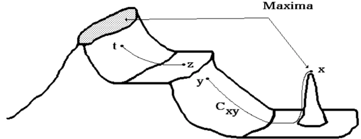
A maximum of f (sometimes called regional maximum) is a summit of the topographic surface G, that is a connected region (but not necessarily reduced to an single point) where it is not possible, starting from any point of this region to reach a higher point (if it exists) of the topographic surface by means of a non descending path (Fig. 1).

Figure 1: Point x belongs to a maximum because, starting from this point, it is impossible

to reach a higher point as y by following a non descending Path. Cxy is not a non

descending path. On the contrary, z does not belong to a maximum because the path Czt

joining z to a higher point t is non descending.

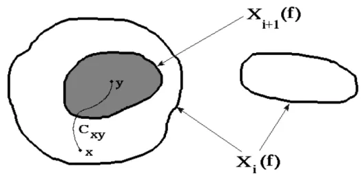
A threshold Xi(f) at level i of a function f defined on E is made of the points of E such that:

Xi(f)= x c E : f(x) m i

The geodesic reconstruction RX(Y) of a set X by a marker set Y (Y _ X ) is made of all the connected components of X which are marked by Y.

The maxima of a function f can be obtained by means of a geodesic reconstruction. Let us consider the various thresholds of f. A maximum of the function at altitude i (if it exists) will be a connected component of the threshold Xi(f) of f containing no connected component of any threshold Xj(f) where j>i. Indeed, suppose that it is not true. Therefore, there exists a path connecting any point of the aforementioned connected component of Xi(f) to any point of the connected component of Xj(f) contained in the previous one (Fig. 2). Let us take

. Then path is the projection of a non descending path on the graph G of f. So, x

j=i+1 cxy

cannot belong to a maximum, which proves the proposition.

So, a maximum at altitude i corresponds to a connected component of Xi(f) which cannot be rebuilt by Xi+1(f) and the set M (f) of all the maxima of f can be defined as:

M(f)=

4

i Xi(f)\RXi(f)[Xi+1(f)] Let us write this formula differently. We know that:

RXi(f)[Xi+1(f)]=RXi(f)[Xi(f−1)]=Xi[Rf(f−1)]

That is:

M(f)=

4

i[Xi(f) 3 Xi c_(R

f(f−1))] This can be written as (see [4]):

M(f)=Xi[f−Rf(f−1)]

Maxima of f are made of points of E where f−Rf(f−1) is strictly positive [2]. This function taking only two values 0 or 1 is also the indicator function kM(f) of the maxima of f.

Minima m(f) of f can be obtained in a similar way by simply using the dual reconstruction R&. We get:

km(f)=Rf

&

(f+1)−f

Figure 2: The right connected component of Xi is a maximum as it cannot be rebuilt by any

connected component of Xi+1 (it does not contain such a component).

3. Algorithmic definition of a h-maximum

The implementation of this operator in the MAMBA image library is straightforward (see the appendix). Moreover, this implementation has been extended by introducing a parameter h for the constant value which is subtracted from f. When this parameter is set to 1 (its default value), we obtain the classical maxima of f. But when h is greater than 1, the connected components of the set resulting of the operation are called h-maxima.

However, characterizing the points which belong to this set is not easy. In fact, this operator is misleading as it does not produce any maximum of height h as its name would suggest. To better understand this general operator, it is interesting to change the definition of a maximum. This new definition is the following:

A point z of the graph of f belongs to a maximum if and only if any non descending path Czz∏

starting from z has a maximum height equal to 0.

This definition is interesting because, contrary to the previous one, there is no need to look for all the points at a higher altitude to check if they are reachable or not by a non descending path.

This definition allows also to simply characterize the points which belong to the set obtained by the h-maximum operator.

A point z of the graph of f belongs to a h-maximum if and only if any non descending path starting from z has a maximum height equal to (h-1).

Czz∏

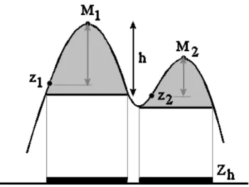
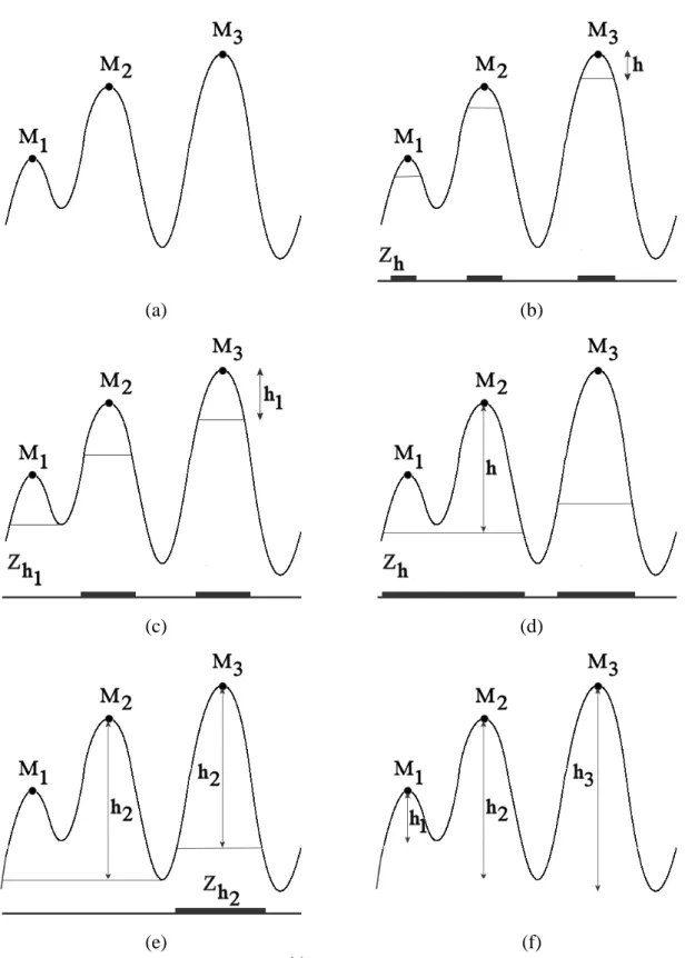
Figure 3: Two maxima M1 and M2 are contained in Zh. But the height of M1 is larger than

h, whilst the height of M2 is lower than h. In both cases, and are at a vertical distancez1 z2

lower than h from these respective maxima.

In other words, the maxima operator in the MAMBA image library provides a set Zh made of all the points x of E for which the corresponding points z=(x, f(x)) on the graph G are at a vertical distance less than h to a maximum of f. However, this set Zh does not mark the maxima of f with a height lower than h. On the contrary, as it can be shown in Fig. 3, some detected domes of the graph G of f correspond to maxima of height larger than h, whilst other correspond to maxima of height lower than h. Moreover, when h increases, the set Zh increases too. The operator is extensive:

h<h∏ u Zh _ Zh∏

So, the domes of f tend to merge when h increases.

Let us denote by rh(f) the operator Rf(f−h). An interesting property of this operator is its distributivity with respect to addition. Indeed, we can show that:

rh1+h2(f)=rh2(rh1(f))=rh2(f) ) rh1(f)

This can be proved by using the thresholds of rh(f). Let us consider a threshold Xi(rh(f)) at level i of the function rh(f). Each connected component (c.c. in brief) of Xi(rh(f)) is obtained by a geodesic reconstruction from at least a marker made of a c.c. of Xi+h(f). Each c.c. of

is also equal to the c.c. of which contains the marker. Let us prove that

Xi(rh(f)) Xi(f) rh(f)

can be iterated. For this, we just need to prove that each c.c. of Xi(rh2 ) rh1) is also a c.c. of then, that each c.c. of is a c.c. of .

Each c.c. of Xi(rh2) rh1) is marked by a c.c. of Xi+h2(rh1). This c.c. is itself marked by a c.c. of . Therefore, as this latter c.c. marks a c.c. of , we have:

Xi+h1+h2(f) Xi(rh1+h2)

Xi(rh2 ) rh1) _ Xi(rh1+h2)

Each c.c. of Xi(rh1+h2) is marked by a c.c. of Xi+h1+h2(f). But this c.c. marks a c.c. of Xi+h2(rh1). And this c.c. marks a c.c. of Xi(rh2 ) rh1). Therefore, we have:

, Q.E.D.

Xi(rh1+h2) _ Xi(rh2) rh1)

4. Height of a maximum (depth of a minimum)

In the sequel, the notion of altitude will be used for introducing some definitions and algorithms. It is important to not mix up these two concepts: altitude and height. The altitude of a point z(x, f(x)) of the graph of f is simply the value f(x). The height of z (which is supposed to belong to a maximum) is, as it has been shown previously, a more complex notion which will be discussed in this section.

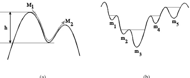
As the operator is unable to provide a satisfactory definition of the height of a maximum,rh other solutions must be explored. The first one could be to define the height of a maximum as the minimal vertical distance one must go down, starting from this maximum to reach another maximum (Fig. 4a). If there exists no other maximum (f has a unique maximum), the height of this maximum is simply equal to the difference between the maximum and minimum values of f.

Figure 4: The height h of the maximum M1 corresponds to the minimal vertical distance

one must go down to reach any other maximum (M2 in this example) (a). Applied to

minima, this definition corresponds to the depth of the corresponding lower catchment

basin, which is far from being satisfactory for minimum m3 (b).

(b) (a)

Applied to minima, this definition of the depth of a minimum corresponds to the height of the lower catchment basin associated to this minimum [3]. We know how to obtain these lower catchment basins by means of a geodesic dual reconstruction using the watershed transform. However, this definition is again not satisfactory. Indeed, as it is illustrated in Fig. 4b, this

depth is almost the same for all the minima of the drawn structure, which is far from being appropriate for the deepest minimum.

Figure 5: Evolution of the function rh(f) of the initial function f (a) when h increases and

relationships between its maxima and the maxima Zh of rh (b). h1 is the dynamics of M1

(c), h2 the dynamics of M2 (e). Finally, h3 is the dynamics of M3. It also corresponds to the

dynamics of f (f). (f) (e) (d) (c) (b) (a)

A better definition of the height of a maximum can be obtained by observing the evolution of the function when h increases and especially by observing its maxima. Let us consider therh function f in Fig. 5a, which shows three maxima, M1, M2 and M3. Successive rh transforms can be applied to f with increasing values of h. Let us also extract the maxima of each rh transform. We can see in Fig. 5b that, at the beginning, all the maxima of f are included in maxima of rh. Then, when h is equal to h1, the first maximum M1 of f is not included anymore in a maximum of rh1 (Fig. 5c). If we increase h, M2 and M3 continue to be marked by maxima of . For a higher value of h, rh M1 is again marked by a maximum of (the samerh maximum also includes M2, Fig. 5d).

Then, when h is equal to h2 (Fig. 5e), the maximum M2 ceases to be included in a maximum of rh2 (this is also the case for M1, although it is not the first time this event occurs). The values h1 and h2 associated to the maxima M1 and M2 respectively (Fig. 5f) are named dynamics of these maxima [6]. It can be shown that the dynamics of a maximum M of a function f is equal to the minimal vertical distance one must go down, starting from this maximum to reach a maximum at a higher altitude than M. When M is the highest maximum, its dynamics is equal to the difference between the maximum and minimum values of f. This value is sometimes defined as the dynamics of the image (it is also called oscillation of the function f ).

So, a small change in the definition (considering a higher maximum instead of any maximum) leads to a much better definition of the height of a maximum as illustrated in Fig. 5f.

Therefore, it is more natural to define the height of a maximum as the value of its dynamics. The same notion can obviously be defined for the minima of an image: the dynamics of a minimum is equal to its depth.

The dynamics of a maximum is not a local attribute which can be determined simply by exploring its surroundings as the maximum which determines the value of the dynamics may be far from the first maximum. Therefore, calculating rapidly the dynamics of all the maxima of an image is not simple. There exists, however, an implementation based on hierarchical queues (described in [6]). Fortunately, in most cases, it is not necessary to calculate the dynamics of all the maxima. We just need to extract those maxima with a height or dynamics higher than or equal to a given value h.

Obtaining those maxima with a dynamics larger than (h - 1) is very easy. They are produced by a simple threshold at level h of the function f−rh(f).

We shall not give the proof of this here (it can be found in [6]), but we can intuitively see why it is true by looking at Fig. 5c. As a matter of fact, when a maximum ceases to be marked, the corresponding part of the function f−rh(f) also ceases to increase and its maximal value is lower than h. Even if the maximum is marked again later on (Fig. 5d), there is a gap in the increase of f−rh(f) which will never be filled in.

These operators (for maxima and minima) are defined in the appendix (they are named

maxDynamics and minDynamics). Note the tiny difference between these operators and the maxima/minima operators (level of the final threshold).

5. Robustness of the dynamics

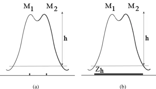
The major drawback of the dynamics lies in its great sensitivity to noise and to small variations of grey levels. One particular drawback has been discussed in [6] and is illustrated in Fig. 6a. When two or more relatively closed maxima are at the same altitude, their dynamics is the same and may be quite high. However, remind that the maxima or minima are widely used to provide markers for the watershed segmentation. Therefore, using extrema of high dynamics to provide these markers may lead to multiple markings of the same salient regions and then to over-segmentations.

Figure 6: The two maxima M1 and M2 have the same altitude and their dynamics are also

equal and higher than h. Selecting these maxima as markers leads to a double marking of

the corresponding salient dome (a). Using the maxima of rh(f) instead produces a single

marker (b).

(a) (b)

There exists solutions to overcome this problem (see [6]). Among them, one of the simplest ones consists in using the maxima of the function rh(f) as markers (or the minima of rh ).

&_(f)

Each maximum contains at least one maximum of the initial function f with a dynamics higher than h. But all the maxima of f which are contained in a single maximum of rh(f) correspond to the maxima which were wrongly separated in the previous example (Fig. 6b). Therefore, using the maxima of rh(f) (or the minima of rh ) prevents over-segmentations in

&_(f)

the watershed transform

These operators have also been added to the appendix (highMaxima, deepMinima).

6. Use of extrema in geodesic reconstructions

To end up this review, let us recall a well-known property of the maxima (or minima) of an image f. If M is the set of all the maxima of f, we can define the valued indicator function of these maxima as the function m equal to:

m(x)=min(f) if x " M

and been respectively the maximal and minimal values taken by f (usely 255 max(f) min(f)

and 0 if f is a 8-bit grey scale image).

Then g=m . f is the function where each maximum belonging to M is valued by its altitude. We know that:

f=Rg(f)

It is very easy to prove this equality. The same property holds with the minima of f and the dual reconstruction.

Now, it is possible to obtain partial reconstructions of f by selecting any subset M’ of M. We have:

m∏(x)=max(f) if x c M∏

m∏(x)=min(f) if x " M∏ The partial reconstruction operator _☞M∏(f) is equal to:

☞M∏(f)=R_m∏_.f(f)

It is also possible to define partial reconstructions by using the dual reconstruction operator and by selecting a specific subset among the minima of the initial image f.

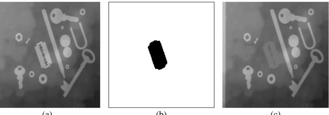
These operators can be useful for designing specific filters (Fig. 7), for a better detection of differences between similar images.

Figure 7: The initial image (a) is rebuilt by taking only those maxima which are outside the marker set (b). The result is shown in (c).

(c) (b)

(a)

A general implementation of these operators can be found in the appendix. They are named

maxPartialBuild and minPartialBuild. They both use a binary set which acts as a mask. Only

maxima (or minima) which fall inside the mask are used for reconstructions.

7. References

[1] BEUCHER Nicolas: MAMBA documentation,(mambaApi Reference Manual). Web documents (available at http://www.mamba-image.org), 2009-2011.

[2] BEUCHER Serge: Segmentation d'Images et Morphologie Mathématique. Doctorate Thesis, Ecole des Mines de Paris, Cahiers du Centre de Morphologie Mathématique, Fascicule n° 10, Juin 1990.

[3] BEUCHER Serge, MARCOTEGUI Beatriz: P algorithm, a dramatic enhancement of the waterfall transformation. CMM/Mines ParisTech publication, 86 pages. September 2009. [4] BEUCHER Serge: About a problem of definition of the geodesic erosion CMM/Mines ParisTech publication, (http://hal.archives-ouvertes.fr), September 2011

[5] BEUCHER Serge: Geodesy and Geodesic Transformations. Lecture slides, Mines ParisTech Mathematical Morphology Course, November 2012.

[6] GRIMAUD Michel: La Géodésie Numérique en Morphologie Mathématique. Application à la Détection Automatique de Microcalcifications en Mammographie Numérique. Doctorate Thesis, Paris School of Mines, December 1991.

.

This document is copyrighted under the Creative Commons "Attribution Non-Commercial No Derivatives" license. For terms of use, see http://creativecommons.org/about/licenses/

8. Appendix

This appendix contains the MAMBA source code for the operators described in this document. The first two operators (maxima and minima) are already contained in the geodesy.py module. The others are gathered in a new module, extrema.py, available at:

http://cmm.ensmp.fr/~beucher/Mamba/extrema.py

"""

This module provides a set of operators dealing with maxima and minima of a function. New operators linked to the notion od dynamics are provided. This module uses Mamba functions available in geodesy.py.

it works with imageMb instances as defined in mamba. """

# Contributor: Serge BEUCHER import mamba

import mambaComposed as mC

def minima(imIn, imOut, h=1, grid=mamba.DEFAULT_GRID): """

Computes the h-minima of 'imIn' using a dual build operation and puts the result in 'imOut'. When ‘h’ is equal to 1 (default value), the operator provides

the minima of ‘imIn’.

Grid used by the dual build operation can be specified by 'grid'.

Only works with greyscale images as input. 'imOut' must be binary. """

imWrk = mamba.imageMb(imIn) mamba.addConst(imIn, h, imWrk) mC.dualBuild(imIn, imWrk, grid=grid) mamba.sub(imWrk, imIn, imWrk)

mamba.threshold(imWrk, imOut, 1, mamba.computeMaxRange(imIn)[1]) def maxima(imIn, imOut, h=1, grid=mamba.DEFAULT_GRID):

"""

Computes the h-maxima of 'imIn' using a build operation and puts the result in 'ImOut'. When ‘h’ is equal to 1 (default value), the operator provides the minima of ‘imIn’.

Grid used by the build operation can be specified by 'grid'.

Only works with greyscale images as input. 'imOut' must be binary. """

imWrk = mamba.imageMb(imIn) mamba.subConst(imIn, h, imWrk) mC.build(imIn, imWrk, grid=grid) mamba.sub(imIn, imWrk, imWrk)

mamba.threshold(imWrk, imOut, 1, mamba.computeMaxRange(imIn)[1]) def minDynamics(imIn, imOut, h, grid=mamba.DEFAULT_GRID):

"""

Extracts the minima of 'imIn' with a dynamics higher or equal to 'h' and puts the result in 'imOut'.

Grid used by the dual build operation can be specified by 'grid'.

Only works with greyscale images as input. 'imOut' must be binary. """

imWrk = mamba.imageMb(imIn) mamba.addConst(imIn, h, imWrk) mC.dualBuild(imIn, imWrk, grid=grid) mamba.sub(imWrk, imIn, imWrk)

mamba.threshold(imWrk, imOut, h, mamba.computeMaxRange(imIn)[1])

def maxDynamics(imIn, imOut, h, grid=mamba.DEFAULT_GRID): """

Extracts the maxima of 'imIn' with a dynamics higher or equal to 'h' and puts the result in 'imOut'.

Grid used by the dual build operation can be specified by 'grid'.

"""

imWrk = mamba.imageMb(imIn) mamba.subConst(imIn, h, imWrk) mC.build(imIn, imWrk, grid=grid) mamba.sub(imIn, imWrk, imWrk)

mamba.threshold(imWrk, imOut, h, mamba.computeMaxRange(imIn)[1]) def deepMinima(imIn, imOut, h, grid=mamba.DEFAULT_GRID):

"""

Computes the minima of the dual reconstruction of image 'imIn' by imin + h and puts the result in 'imOut'.

Grid used by the dual build operation can be specified by 'grid'.

Only works with greyscale images as input. 'imOut' must be binary. """

imWrk = mamba.imageMb(imIn) mamba.addConst(imIn, h, imWrk) mC.dualBuild(imIn, imWrk, grid=grid) mC.minima(imWrk, imOut, 1, grid=grid)

def highMaxima(imIn, imOut, h, grid=mamba.DEFAULT_GRID): """

Computes the maxima of the reconstruction of image 'imIn' by imin + h and puts the result in 'imOut'.

Grid used by the build operation can be specified by 'grid'.

Only works with greyscale images as input. 'imOut' must be binary. """

imWrk = mamba.imageMb(imIn) mamba.subConst(imIn, h, imWrk) mC.build(imIn, imWrk, grid=grid)

mC. maxima(imWrk, imOut, 1, grid=grid)

def maxPartialBuild(imIn, imMask, imOut, grid=mamba.DEFAULT_GRID): """

Performs the partial reconstruction of 'imIn' with its maxima which are contained in the binary mask 'imMask'. The result is put in 'imOut'.

'imIn' and 'imOut' must be different and greyscale images. """

imWrk = mamba.imageMb(imIn, 1) mC.maxima(imIn, imWrk, 1, grid=grid) mamba.logic(imMask, imWrk, imWrk, "inf")

mamba.convertByMask(imWrk, imOut, 0, mamba.computeMaxRange(imIn)[1]) mamba.logic(imIn, imOut, imOut, "inf")

mC.build(imIn, imOut)

"""

Performs the partial reconstruction of 'imIn' with its minima which are contained in the binary mask 'imMask'. The result is put in 'imOut'.

'imIn' and 'imOut' must be different and greyscale images. """

imWrk = mamba.imageMb(imIn, 1) mC.minima(imIn, imWrk, 1, grid=grid) mamba.logic(imMask, imWrk, imWrk, "inf")

mamba.convertByMask(imWrk, imOut, mamba.computeMaxRange(imIn)[1], 0) mamba.logic(imIn, imOut, imOut, "sup")

mC.dualBuild(imIn, imOut)