Université de Montréal
A Rolling Horizon Approach for the Locomotive
Routing Problem at the Canadian National Railway
Company
par
Hoang Giang Pham
Département d’informatique et de recherche opérationnelle Faculté des arts et des sciences
Mémoire présenté en vue de l’obtention du grade de Maître ès sciences (M.Sc.)
en Informatique et recherche opérationnelle
October 7, 2020
c
Université de Montréal
Faculté des arts et des sciences Ce mémoire intitulé
A Rolling Horizon Approach for the Locomotive Routing
Problem at the Canadian National Railway Company
présenté par
Hoang Giang Pham
a été évalué par un jury composé des personnes suivantes :
Margarida Carvalho (président-rapporteur) Emma Frejinger (directeur de recherche) Jean-François Cordeau (codirecteur) Bernard Gendron (membre du jury)
Résumé
Cette thèse étudie le problème du routage des locomotives qui se pose à la Compagnie des chemins de fer nationaux du Canada (CN) - le plus grand chemin de fer au Canada en termes de revenus et de taille physique de son réseau ferroviaire. Le problème vise à déterminer la séquence des activités de chaque locomotive sur un horizon de planification donné. Dans ce contexte, il faut prendre des décisions liées à l’affectation de locomotives aux trains planifiés en tenant compte des besoins d’entretien des locomotives. D’autres décisions traitant l’envoi de locomotives aux gares par mouvements à vide, les déplacements légers (sans tirer des wagons) et la location de locomotives tierces doivent également être prises en compte. Sur la base d’une formulation de programmation en nombres entiers et d’un réseau espace-temps présentés dans la littérature, nous introduisons une approche par horizon roulant pour trouver des solutions sous-optimales de ce problème dans un temps de calcul acceptable. Une formulation mathématique et un réseau espace-temps issus de la littérature sont adaptés à notre problème. Nous introduisons un nouveau type d’arcs pour le réseau et de nouvelles contraintes pour le modèle pour faire face aux problèmes qui se posent lors de la division de l’horizon de planification en plus petits morceaux. Les expériences numériques sur des instances réelles montrent les avantages et les inconvénients de notre algorithme par rapport à une approche exacte.
mots clés: Problème du Routage des Locomotives, Approche par Horizon Roulant.
Abstract
This thesis addresses the locomotive routing problem arising at the Canadian National Rail-way Company (CN) - the largest railRail-way in Canada in terms of both revenue and the physical size of its rail network. The problem aims to determine the sequence of activities for each locomotive over the planning horizon. Besides assigning locomotives to scheduled trains and considering scheduled locomotive maintenance requirements, the problem also includes other decisions, such as sending locomotives to stations by deadheading, light traveling, and leasing of third-party locomotives. Based on an Integer Programming formulation and a Time-Expanded Network presented in the literature, we introduce a Rolling Horizon Ap-proach (RHA) as a method to find near-optimal solutions of this problem in acceptable computing time. We adapt a mathematical formulation and a space-time network from the literature. We introduce a new type of arcs for the network and new constraints for the model to cope with issues arising when dividing the planning horizon into smaller ones. Computational experiments on real-life instances show the pros and cons of our algorithm when compared to an exact solution approach.
Contents
Résumé . . . . 3 Abstract . . . . 4 List of tables . . . . 7 List of figures . . . . 9 List of abbreviations . . . . 10 Acknowledgements . . . . 11 Chapter 1. Introduction . . . . 12Chapter 2. Literature Review . . . . 15
2.1. The Locomotive Scheduling Problem . . . 15
2.1.1. The Locomotive Assignment Problem . . . 16
2.1.2. The Locomotive Routing Problem . . . 20
2.2. The RHA for Mixed Integer Programming . . . 21
Chapter 3. Problem Definition . . . . 26
3.1. Overview . . . 26
3.2. Data & Constraints . . . 27
Chapter 4. Model and Solution Method . . . . 32
4.1. The Existing Space-time Network . . . 32
4.1.1. Bottom Layer . . . 33
4.1.2. Top Layer & Connecting Layers . . . 35
4.2. The Existing Mathematical Formulation . . . 37
4.3. The Rolling Horizon Approach . . . 40
4.3.2. The Adaptation of the IP Model to the RHA. . . 45
4.3.3. The Rolling Horizon Approach . . . 47
4.3.4. Updating Information in the RHA . . . 54
Chapter 5. Computational Experiments . . . . 67
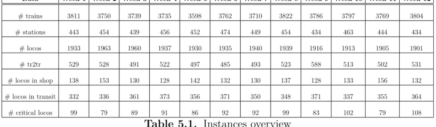
5.1. Instances & Parameter Setting . . . 67
5.2. The Effects of the Planning Horizon and the Roll Period on the Results . . . 69
5.3. The Solution Quality and Computational Time for Longer Time Horizons . . . . 71
Conclusion & Future Work . . . . 76
References . . . . 77
List of tables
4.1 Sets of nodes and arcs in the time-space network . . . 36
4.2 Decision variables in mathematical formulation. . . 37
4.3 Parameters in mathematical formulation . . . 41
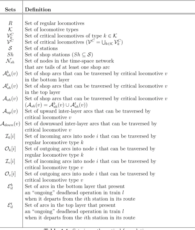
4.4 Sets in mathematical formulation . . . 42
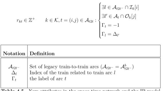
4.5 New attributes in the space-time network and the IP model . . . 47
5.1 Instances overview . . . 67
5.2 The relative difference of the results of the first instance solved by the RHA with the results provided by the exact solution of the IP-based model (%) . . . 69
5.3 Comparison of the objective values of the relaxation solutions provided by CPLEX with the objective values provided by the RHA . . . 71
5.4 Comparison of the results of instances with 8,9-day planning horizon solved by the RHA with the exact solution of the IP-based model . . . 74
5.5 Comparison of the results of instances with 10,11-day planning horizon solved by the RHA with the exact solution of the IP-based model . . . 74
5.6 Comparison of the results of instances with 12,13-day planning horizon solved by the RHA with the exact solution of the IP-based model . . . 75
5.7 Comparison of the results of instances with 14-day planning horizon solved by the RHA with the exact solution of the IP-based model . . . 75
A.1 Optimal solutions of first 6 weeks . . . 80
A.2 Optimal solutions of last 6 weeks . . . 81
A.3 The relative difference of two methods with h = 3, r = 2 (%) . . . 81
A.4 The relative difference of two methods with h = 4, r = 2 (%) . . . 82
A.5 The relative difference of two methods with h = 5, r = 2 (%) . . . 82
A.6 The relative difference of two methods with h = 4, r = 3 (%) . . . 82
A.8 The relative difference of two methods with h = 5, r = 4 (%) . . . 83 A.9 Results of 2-week instances with h = 3, r = 2 . . . 83
List of figures
3.1 Example of RHA illustrations and the notations . . . 27
4.1 Example of the bottom layer in a space-time network with 3 stations. Source: Miranda et al. (2020) . . . 33
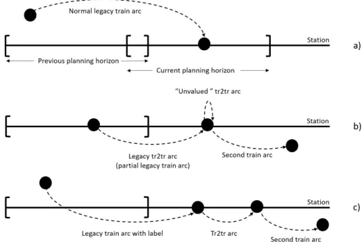
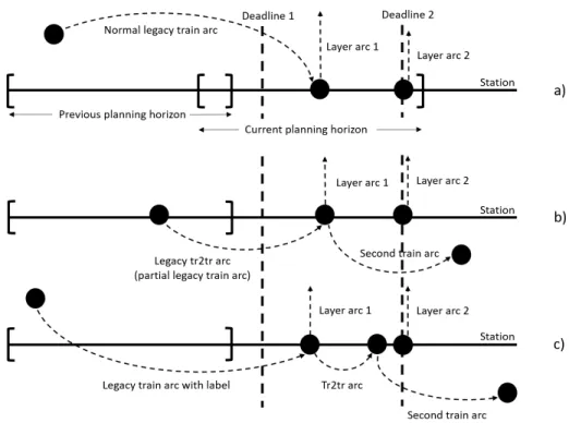
4.2 Legacy train arcs and legacy train-to-train arcs . . . 43
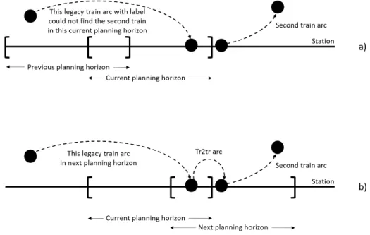
4.3 How to deal with invalid legacy train arc with label . . . 44
List of abbreviations
LAP Locomotive Assignment Problem
LRP Locomotive Routing Problem
RHA Rolling Horizon Approach
Acknowledgements
Foremost, I would like to express the deepest appreciation to my supervisor Prof. Emma Frejinger and my co-supervisor Prof. Jean-François Cordeau for the continuous support of my Master’s study and research, for their patience, motivation, enthusiasm, and immense knowledge. Their guidance not only helped me in all the time of studying and writing of this thesis, but also taught me how to work scientifically in my research career.
Besides my supervisor and my co-supervisor, I would like to thank Dr. Pedro Miranda, for his research that inspired me to begin doing my thesis, insightful explanations about the methodology, significant comments about all the issues, and challenging questions for me to work with.
My sincere thanks also go to Mr. Eric Larsen for helping me to access the real-life data of the Canadian National Railway Company.
Last but not the least, I would like to thank my family: my parents Mrs. Dang Thi Loc and Mr. Pham Hong Truong, for giving birth to me in the first place and supporting me spiritually throughout my life, my younger sister Ms. Pham Thu Trang, for her belief that I deserve to be her elder brother. In memory of my grandmother, I am extremely grateful for her love, prayers, and caring for both my childhood and my future.
Chapter 1
Introduction
Rail transportation is a product of the industrial era, playing a major role in economic development. A massive railway system implemented in North America contributed to it becoming one of the world’s largest economies. Railroads play an essential role in trans-portation of people and goods over long distances not only because of their capacity to carry heavy loads but also because of their speed, safety, and relatively low environmental impact. Canadian National Railway Company (CN) operates Canada’s largest railway and is Canada’s only transcontinental railway company. Its network spans Canada from the At-lantic coast in Nova Scotia to the Pacific coast in British Columbia across about 20,400 route miles (32,831 km) of track. For a Canadian Class I freight railway as CN, several thousand weekly trains are operated by using more than 2,000 locomotives, including both owned and leased ones. The operating and net income of CN was several billion Canadian dollars in 2019. Therefore, most of the planning and scheduling problems arising in railroads involve billions of dollars of resources annually.
Due to the vastness of the worldwide railway system, there are many challenging optimiza-tion problems arising. They were listed as large, relevant and complex issues in Ahuja et al. (2005a), including, e.g., blocking problem, yard location problem, train scheduling problem,
locomotive scheduling problem, maintenance planning problem, train dispatching problem,
and crew scheduling problem.
Among these problems, the locomotive scheduling problem consists in efficiently assigning different types of locomotives to the scheduled trains. This problem can be divided into two problems, namely, the locomotive assignment problem (LAP) and the locomotive routing
problem (LRP). The first one is at the tactical level, where locomotives are classified into
types based on their main physical characteristics, including horsepower, pulling capabilities, weight, number of axles, cost, among others. The second one arises at the operational level, where the activities of individual and uniquely identified locomotives must be specified in detail.
This thesis focuses on the LRP faced by CN and is an extension of the work of Miranda et al. (2020), who introduce a time-expanded formulation to find optimal solutions for the same problem. They propose an exact method to solve optimally 1-week instances of the LRP in an acceptable computing time (about 10-15 minutes). However, if the railway requires to consider a long-term plan such as 10-day or 2-week operational schedules, the problem becomes too hard to solve with the exact approach. Indeed the number of arcs and nodes in the space-time network and the number of variables in the integer programming model dramatically increase when expanding the planning horizon. This is a motivation for us to implement a heuristic rolling horizon method providing good quality solutions.
Inspired by the work of Miranda et al. (2020), this thesis makes the following contribu-tions. First, we modify the space-time network, allowing us to present the LRP corresponding to each sub-instance created by dividing an instance into smaller overlapping time horizons. Maintenance deadlines of critical locomotives and the constraints related to them must be redefined to fit each sub-instance. The Rolling Horizon Approach (RHA) also requires to add a new type of arcs to the network to satisfy one of the most essential operational re-quirements - train-to-train connections, which can be broken when the real-life instances are divided into smaller fragments.
Second, we adapt and implement the IP formulation introduced in Miranda et al. (2020). The adaptations, in terms of both the IP model and the space-time network, are the study of the issues coming from constraints about critical locomotive maintenance deadlines and train-to-train connections. The conflicts, caused by those constraints, must be avoided not only by modifying the existing constraints but also by adding new constraints when switching from one planning horizon to another in the RHA.
Third, we apply the RHA to solve all sub-instances and then collect their solutions to create a final result for each real-life instance. We should note that several activities of the locomotives are not considered in the solution of each sub-instance if they start in a period of time called overlap. The overlap, which begins at the end of the roll period and ends at the end of the planning horizon, is a shared period of time of two consecutive planning horizons. The latest activity of each locomotive, which occurs before and finishes after the end of the roll period, will be recorded for later iterations in the RHA because it directly affects the input of the next planning horizons.
Finally, we analyze computational experiments of 7-day instances to observe all the effects of the overlap and the chosen planning horizons in the RHA. In case of longer time horizon instances, we study the quality of the solution provided by the RHA when compared with the exact IP-based method.
The rest of the thesis is organized as follows. In Chapter 2, we briefly discuss the relevant literature. Chapter 3 provides the problem description, while Chapter 4 describes in detail the space-time network and the IP model. Both of them are modified to adapt to the RHA framework. Extensive computational experiments are carried out and reported in Chapter 5. The detailed computational results are provided in Appendix A.
Chapter 2
Literature Review
We review several works that study the locomotive scheduling problem in Section 2.1. Two main categories of this problem, which are known as the locomotive assignment problem and the locomotive routing problem, are reviewed in Section 2.1.1 and Section 2.1.2 respec-tively. We discuss the Rolling Horizon Approach for decomposing large-scale IP models in Section 2.2.
2.1. The Locomotive Scheduling Problem
Because of the high cost of owning and operating locomotives, the locomotive scheduling
problem plays an essential role in rail transportation. The question of making the most
efficient use of the locomotives has challenged researchers for a few decades. This problem aims to satisfy pulling requirements of the scheduled trains while decreasing the cost of operating locomotives and obeying a variety of constraints, such as fleet-size constraints on different locomotive types, fueling, and maintenance constraints (Ahuja et al.; 2005b; Vaidyanathan et al.; 2008a). Because the problem of real size is large and complex, it is highly essential to employ Operations Research techniques and practical optimization tools to support locomotive scheduling decisions (Ortiz-Astorquiza et al.; 2019).
Studying the surveys of Cordeau et al. (1998) and, more recently, Piu and Speranza (2014), we understand that most models and algorithms focus on solving realistic versions of the LAP. This problem aims to determine a set of locomotive types assigned to each train, the way locomotives will deadhead or light travel in the network, and which train-to-train connections should be created. However, the result of the LAP can not be implemented directly in operation. Therefore, in the context of the locomotive scheduling problem, the LRP is an important problem raised by the railroads at the operational level. The LRP aims to decide detailed operating activities of each locomotive based on the result of the LAP. Despite being essential, publications focusing on the LRP are rather scarce.
2.1.1. The Locomotive Assignment Problem
At the tactical level, the LAP determines how to effectively assign the number of locomo-tives of each type to the scheduled trains while taking into account constraints on the fleet size for each locomotive type, power requirement for each train, compatibility between trains and locomotive types, balanced flow of locomotives through the railroad network. From now on, a set of locomotives assigned to each train in a given schedule is called a consist.
To balance the flow of locomotives through the network, the LAP considers how to move locomotives from stations where they are in surplus of power requirement to other ones with a shortage. Besides relocating locomotives by using them to pull the trains, locomotives may also be attached to the trains without actively pulling, which is called deadheading. They can also travel or pull others in a group of locomotives (without rail cars), which is called
light traveling (Ahuja et al.; 2005b; Vaidyanathan et al.; 2008a). Comparing two types of
re-positioning, we see that light traveling is more flexible than the deadheading, but it is more expensive due to the need of an operational crew.
Other important characteristics to incorporate in the LAP are consist busting and
train-to-train connections. Consist busting is considered when a train arrives at its destination
station. If the consist is busted, the corresponding locomotives become separately available at the station. However, busting is time-consuming and avoided when possible. It is not essential to re-assign consists for back-and-forth trains, or trains that have changed their ID in the given schedule but are physically the same. If two trains require the same set of locomotive types and the destination of the first train is the departure of the second train, the consist of the arriving train can be used for the departing one. In those cases, consist busting is replaced by train-to-train connection. As pointed out by Ahuja et al. (2005a), Ahuja et al. (2005b), Vaidyanathan et al. (2008a), the train-to-train connections can decrease train delays and crew time to decouple and move locomotives individually.
At the operational level, maintenance and fueling requirements of individual locomotives might reduce the locomotive availability over the planning horizon. Furthermore, in real life, planners are concerned with assigning locomotive units to trains, rather than locomotive types since the output of solving the LAP is not directly implementable. Thus, the LRP arises at the operational level to further refine and adjust the locomotive assignment plan. In this thesis, the LRP, an extension of the works of Ortiz-Astorquiza et al. (2019) and Miranda et al. (2020), determines the sequences of activities operated by each locomotive, such as pulling trains, taking part in train-to-train connections, light traveling, deadheading, and undergoing maintenance.
Among these activities, only pulling trains and deciding train-to-train connections are dependent on the consist assignment in the output of the LAP. The deadheads and light travels must be reassigned because of the impact of maintenance operations on the flow of individual locomotives over the network (Miranda et al.; 2020). The maintenance operations have a significant impact on the locomotive routing. Each locomotive must be maintained periodically. For example, locomotives have to pass through maintenance every 92 days in North America according to the law. Furthermore, the railroad companies may set deadlines to send locomotives to the shop for semi-yearly, yearly, or quadrennial major revisions and mechanical repairs. The locomotives cannot pull trains or travel on their own (i.e., light travel) if they missed their maintenance deadlines. In that case, they will be turned off and deadheaded to a shop for checkup (Bouzaiene-Ayari et al.; 2016). At each shop station, locomotives may be served right after arriving or have to wait in line for a spot since each shop has limited capacity and is frequently congested. An imbalance in power availability across the network may be created by locomotive unavailability. Therefore, railway companies prefer sending locomotives to the shops, neither too early nor too late, while maximizing their productivity.
In addition to classify problems based on planning levels as mentioned above, the LAPs and the LRPs may be distinguished by the number of pulling locomotives a train may require (Vaidyanathan et al.; 2008a). The problem can be modeled as a “single-locomotive model” if each train needs a single pulling locomotive. If some trains require more than one pulling locomotive, the problem falls into the “multiple locomotive model” category. In this thesis, the LRP is modeled by a “multiple locomotive model” because we must assign a set of locomotives (consist) to each train based on the consist provided by the result of the LAP.
Generally, “single-locomotive” problems are easier to solve than “multiple locomotive” ones. The single-locomotive model category can be divided into two types by considering how many locomotive types the model requires. Forbes et al. (1991) argue that the problem becomes similar to the single-depot bus (vehicle) scheduling problem if only one locomo-tive type is required. Otherwise, the problem can be considered as the multiple depot bus (vehicle) scheduling problem.
Wright (1989) implements three algorithms to solve the problem with multiple locomotive types: the first is a deterministic algorithm to find a feasible solution, the second is a local improvement method, and the third is a simulated annealing algorithm. Although the first valid solution for large scale version of multiple locomotive model is found, the author does not recommend the use of the procedure for real-life applications because the solution does not take into account the fleet size constraints.
Inspired by the work of Wright (1989), Forbes et al. (1991) introduce a model based on an integer linear program equivalent to a multi-commodity flow formulation. The model, where each commodity represents a locomotive type, obtains an exact solution for instances of 25-200 trains. It is a significant improvement over the method proposed by Wright (1989) because the model is able to take into account the fleet size constraints.
More recently, Fugenschuh et al. (2006) extend the work of Forbes et al. (1991) by adding several new aspects: cyclic train departures, time windows on start and arrival times, transfer of wagons among trains. Two linear integer programming problems with fixed and flexible start and arrival times are introduced. While the first model is solved to optimality by using CPLEX directly, a combination of a randomized parameterized greedy (PGreedy) heuristic and a special purpose reformulation to improve the formulation of the problem is implemented before using CPLEX to cope with the second one.
The most sophisticated version of the LAP (or the LRP) occurs when each train requires a consist instead of a single pulling locomotive. Florian et al. (1976) is the first to study this version of the problem. The authors consider a freight train problem arising at CN. It is formulated as a multi-commodity network flow problem. The objective is to minimize the capital investment and the maintenance costs while assigning a sufficient number of locomotives of different types to satisfy the motive power requirements of each train. A Benders decomposition method is proposed to deal with the weekly train schedule. However, their implementation can not solve the problem to optimality and can be acceptable for medium-sized problems but not for large ones.
Cordeau et al. (2000) propose an IP formulation to deal with the simultaneous assign-ment of locomotives and rail cars in the context of passenger transportation. It is formu-lated as a multi-commodity flow problem on a space-time network. In the network, each node represents an event, i.e., arrival, departure, and repositioning of a unit. Each arc performs an activity of scheduled train, such as operating, repositioning, and waiting. An exact algorithm, based on the Benders decomposition approach, is introduced to solve a set of nine instances obtained from VIA Rail Canada. Compared with three other solution methods, namely, Lagrangian relaxation, simplex-based branch-and-bound algorithm, and Dantzig–Wolfe decomposition, the authors show that the method based on Benders decom-position finds optimal solutions within a short computation time. However, this model is not sophisticated enough to be used in practice because it does not consider constraints that are important in practice. Thus, in Cordeau et al. (2001), it is modified by incorporating a much broader set of constraints and possibilities required in a commercial application.
The problem introduced in Cordeau et al. (2001) is an extended version of the one in Cordeau et al. (2000). A large-scale IP model and a heuristic approach based on column generation are introduced to solve this real-life problem. The solution, provided by applying a heuristic branch-and-bound method in which the linear relaxation lower bounds are com-puted by column generation, has been successfully implemented at VIA Rail. The algorithm can satisfy a long-term planning horizon and find a good quality solution in a few hours of computation.
Vaidyanathan et al. (2008a) introduce two formulations: consist formulation, and hybrid
formulation for the locomotive planning problem arising at CSX Transportation (a Class I
US Railroad). They consider an extension of the problem studied in Ahuja et al. (2005b), wherein all the real-world constraints are not incorporated to generate a fully implementable
solution. In Vaidyanathan et al. (2008a), the authors not only add new constraints to
the problem desired by locomotive directors, but also develop additional formulations to transition their solutions to practice. The major contribution of the paper is a new approach for routing consists instead of routing individual locomotives. The computational tests show that if good consists are created, even though the routing of consists seems to restrict the solution space, high-quality solutions are provided by the consist formulation and they are easier to implement for locomotive dispatchers. The consist formulation runs faster and is more robust than the hybrid formulation and the flow-based models in Ahuja et al. (2005b), while the objective value of the hybrid formulation is better (by 5%) than the one of the consist formulation (the flow-based models cannot converge to a feasible solution after 10 hours of running time).
Ortiz-Astorquiza et al. (2019) develop mathematical optimization models and Benders-based solution algorithms to find high-quality solution for the LAP arising at CN. Two IP formulations, namely Locomotives-Based Formulation (LBF) and Consist-and-Locomotive Flow-Based Formulation (CLF), are introduced. The results of extensive computational experiments show that the CLF model provides a good solution in reasonable running time when solved with a general-purpose solver. The performances of those formulations are also improved by two versions of an algorithm based on Benders decomposition. Those versions significantly reduce the CPU time to obtain a first solution. The solution analysis shows that the enhanced model provides a 25% reduction in the number of locomotives compared with the locomotive schedule used in actual operations. To sum up, the authors argue that the proposed model (CLF) is well-suited to provide good solutions for the LAP with significant cost and running time reduction.
2.1.2. The Locomotive Routing Problem
With the idea of solving a series of small overlapping instances extracted from the original problem, Ziarati et al. (1997) extend the work of Florian et al. (1976) and achieve a reduction of 7−7.5% in both the number of locomotives in use and power consumption when studying a problem arising at CN. They define this problem as a LAP where each train requires sufficient power during its operation, and locomotives having maintenance requests must be sent to the shop within a given time limit. Due to the presence of maintenance constraints for individual locomotives, we can consider this problem as an LRP at the operational level. The authors introduce a multi-commodity network flow-based model and then decompose the model into a master problem and a set of sub-problems using the Dantzig-Wolfe decomposition technique. A branch-and-bound procedure, where the linear relaxation at each node is solved by column generation, is used to generate integer feasible solutions.
In Ziarati et al. (1999), the authors extend the work in Ziarati et al. (1997) with a cutting plane approach. First, a train whose demand is fulfilled by two locomotive types is selected. Then, a branching decision is imposed on forbidding the assignment of other locomotive types to this train. Finally, the appropriate cutting planes are added for this train to strengthen the formulation. They use a RHA in the computational experiments due to the large size of the instance, which contains thousands of trains and locomotives. By using cutting planes, the integrality gap is decreased by an average of 23%. Comparisons with CN’s solutions show a reduction of 11 locomotives or, equivalently, a 1.1% saving.
To complement previous research in Vaidyanathan et al. (2008a) and Ahuja et al. (2005b), Vaidyanathan et al. (2008b) study the LRP problem faced by CSX Transportation, a major U.S. railroad company. This problem aims to determine paths of individual locomotives whose actions are limited by fueling and maintenance constraints. These constraints require each locomotive to visit a fueling station and a shop before a given number of miles of travel. The authors define the sequence of trains that the locomotive takes between fueling stops as a fuel string and the sequence of trains that the locomotive takes between servicing stops as a service string. Then, the enumerated paths are used as input parameters for an integer program that aims to decompose the locomotive assignment into flows on paths. This integer programming problem with millions of decision variables cannot be solved using a commercial solver. Therefore, they develop a fast aggregation-disaggregation based algorithm to solve this formulation within a few minutes. The computational experiments show a less than 2.2% optimality gap.
Bouzaiene-Ayari et al. (2016) introduce a suite of models, ranging from single and multi-commodity flow models to a multi-attribute model, which have been successfully imple-mented at Norfolk Southern. While the single and multi-commodity flow models can be solved using commercial integer programming solvers, the multi-attribute resource alloca-tion model is solved by approximate dynamic programming (ADP). At the strategic level, all locomotives are considered at the same time in a single commodity flow model, wherein locomotives are grouped into a single type, and their flows (through the shop and foreign power) are approximated at an aggregate level. At the operational level, locomotives are grouped into four classes (high and low horsepower, high and low adhesion) as the input of the multi-commodity flow model. Small instances can be solved using CPLEX, but the dramatic growth in run times forces the authors to implement a multi-attribute resource al-location model when increasing the size of the data. By using ADP to solve the third model, they demonstrate how efficiently to implement ADP for both deterministic and stochastic models that capture locomotives and trains at a very high level of detail. Although ADP is suitable to handle high levels of details, it does not globally optimize the locomotives flow on the network over time.
Miranda et al. (2020) study the LRP arising at CN, wherein repositioning locomotives through deadheads, light travels, and leasing of third-party locomotives are considered be-sides maintenance operations. The authors propose an IP formulation to solve the integer multi-commodity flow problem with side constraints, based on a two-layer time-expanded network representation of the problem. In the IP model introduced in Miranda et al. (2020), regular locomotives are grouped into types, while critical locomotives are considered indi-vidually. By doing this, their model is reduced in size and can be solved optimally within reasonable computing times. As we show in Section 5.3, the method introduced in that paper can solve to optimality all instances with a planning horizon up to 10 days. However, computing times dramatically increase when expanding the planning period. For this reason, Miranda et al. (2020) inspires us to implement the RHA, with the purpose of decreasing the computing time and providing near-optimal solutions.
2.2. The RHA for Mixed Integer Programming
Mathematical programming, especially IP, has been widely used for modeling the sched-uling and planning problems because of its flexibility and extensive modeling capability, as well as the existence of powerful off-the-shelf solvers. However, NP-hard problems remain challenging to solve. In this thesis, we are interested in using the mathematical formulation
proposed by Miranda et al. (2020) for an optimization problem with a certain time horizon. It is a large-scale IP model and its size increases dramatically when the length of the time horizon increases. An efficient method to decompose this IP model and provide near-optimal solutions with more reasonable computing time is to solve smaller problem within a rolling horizon framework. In the following we provide a number of examples implementing the RHA to solve problems from various areas of application.
In the literature, the RHA is often used in manufacturing scheduling, as well as in other areas (see, e.g., the survey in Chand et al.; 2002). Here, the rolling horizons are implemented routinely to update or revise schedules, estimate a part of the future plan based on reliable and recent data. The basic idea is to repeatedly solve a MIP, which covers a short time horizon. An overlap between two consecutive short time horizons creates an opportunity to make a better overview in the future plan, and the result in this period does not count for the final result. The decision in the overlap will be re-optimized in order to adapt all changes in the coming manufacturing plan. When all days of the planning horizon have been considered in at least one MIP, the overall problem is completely solved.
Baker and Peterson (1979) argue the importance of using rolling schedules in production planning due to their representation of the practical means by which analysis is converted to action in dynamic problems. Even when the optimal solution is found for a long time horizon, that solution is seldom directly implemented in real-life without revision. When new information becomes available, it is more common to revise the planning and modify the previous solution to adapt to the changes in data. Baker (1977) was among the first to test the effectiveness of schedules obtained from a RHA. The author shows that the longer the planning horizon is, the better the rolling horizon performance of static models. In Baker and Peterson (1979), the authors prove that in almost cases, longer planning horizons provide monotonic improvements in performance, but tend to be more challenging to solve. Several powerful algorithms for solving rolling horizon problems were introduced in Stauf-fer and Liebling (1997), Dimitriadis et al. (1997), Mercé and Fontan (2003), Araujo et al. (2007).
Since a long time horizon needs to be considered in the railway operation, it is not easy to obtain an optimal or even a near-optimal solution. To overcome this issue, the RHA is considered as an efficient way to solve the LRP in Ziarati et al. (1997) and Ziarati et al. (1999). That is, they divide the whole LRP into several stages, where each stage is only for train services in a short period. Only the plan for the near future is updated and executed at each stage. By this practice, a RHA, which helps decrease the computation time and provides a nearly optimal solution, is utilized to decompose the LRP.
Additionally, the RHA is also applied to the railway rescheduling area, wherein the railway dispatchers usually reschedule train services gradually, such as the high-speed train system. The literature on that subject is shown in the papers of Nielsen et al. (2012), Quaglietta et al. (2013), Pellegrini et al. (2014), and Zhan et al. (2016).
Nielsen et al. (2012) study real-time disruption management of railway rolling stock in the Netherlands. A generic framework is introduced to deal with disruptions of railway rolling stock schedules. They propose an online combinatorial decision problem, where a sequence of information updates represent the uncertainty of a disruption. To decompose the problem and to reduce the computation time, their RHA is described as follows: rolling stock decisions are only considered if they are within a specific time horizon from the time of rescheduling. The experimental results shows that the RHA can handle the rolling stock during a disruption with minor effects for the shunting plans. With the short computation times, the RHA is indicated as the right candidate for being used in the decision support system for rolling stock rescheduling.
Quaglietta et al. (2013) introduce a framework that couples the state-of-the-art dispatch-ing system ROMA (Railway traffic Optimization by Means of Alternative graphs) devel-oped by D’Ariano (2009) with the microscopic simulation model of railway networks, called EGTRAIN, in Quaglietta and Punzo (2013). A RHA is implemented to perform this inte-gration. The authors also refer to different disturbed traffic scenarios created by sampling train entrance delays and dwell times within a typical Monte-Carlo scheme. The results of this study show that the instability of plans increases over time as stochastic disturbances propagate on the network independently from the length of the prediction horizon. Short horizons provide more solid plans in terms of reordering, but probably a lower performance in recovering delays. However, longer prediction horizons focus on reordering to reduce constant delays but make plans more unstable concerning the reordering.
Pellegrini et al. (2014) propose a mixed-integer linear programming formulation for tack-ling the real-time railway traffic management problem arising in two control areas in France. This formulation can model either the route-lock sectional-release interlocking system (SR) or the route-lock route-release one (RR) by applying two different alternative objective func-tions. Following that, they introduce SR and RR formulation, respectively. For both al-ternative formulations, a rolling-horizon framework is implemented to perform subsequently for scheduling and routing trains during a long time horizon. In this framework, the time interval for a single optimization advances throughout the day. Besides, previously made de-cisions can be either modifiable or not in order to ensure the compatibility of two dede-cisions made in two consecutive time intervals.
Zhan et al. (2016) study the high-speed train rescheduling problem where one track of a double-track train is temporarily unavailable. Three MILP models are introduced to formulated three practical train rescheduling strategies, and then they are solved by a RHA. The results obtained by the RHA are compared with those obtained by the centralized approach. Their analysis shows that the gaps between the solutions provided by the RHA and those achieved by the centralized approach are relatively small for disruption instances with short durations. The most significant gap is around 20%, but the average gaps are smaller than 3%. For disruption instances with longer durations, the gaps are not far from the gaps mentioned above. This study proves that the disposition timetables solved by the RHA are near-optimal, and the RHA is quite efficient in obtaining a reasonable disposition timetable.
Expanding the work in Lai et al. (2008a), Lai et al. (2008b) introduce a rolling horizon model to cope with the aerodynamic efficiency of intermodal freight trains with uncertainty. A static model, formulated as a MIP, is developed to optimize the load placement on a se-quence of intermodal scheduled trains. The authors also implement a dynamic model, which is a modification of the static model with exponentially decreasing weights assigned to the objective functions of future trains, to account for incomplete or uncertain information on later trains and incoming loads. A rolling horizon scheme, in which future trains are consid-ered simultaneously with the current train, is used to deal with the challenge coming from the dynamic model. The experimental result of the dynamic model under the performance of the rolling horizon framework is analyzed based on two simulations: a terminal with a uniform arrival rate of incoming loads and a terminal with a nonuniform arrival rate of in-coming loads. For the first simulation, the rolling horizon provides solutions close to the known optimum (relative optimality gap between 0.1% − 3%) after 600 CPU seconds. The results of the second simulation are largely similar to uniform operations, and the rolling horizon performs an 8.6% benefit equivalent to approximately 700,000 gallons of fuel savings per year.
Samà et al. (2013) show that the RHA is also efficient in aircraft scheduling. They consider the real-time problem of scheduling aircraft in two major Italian Terminal Control Areas where airborne decisions need to be taken in given time horizons of traffic prediction. An alternative graph formulation formulates their problem, and a RHA is implemented to control busy traffic situations when a large number of aircraft are delayed. A Branch-and-Bound algorithm (BB) is compared with a First Come First Served rule presenting the dispatchers’ behaviors in real-life operation. In terms of delay and travel time minimization, the RHA solved by BB provides better results than First Come First Served rule. Moreover,
BB requires fewer changes of aircraft schedule than First Come First Served during consecu-tive look-ahead periods. Therefore, the result of BB is more stable and easier to implement in operation than First Come First Served’s one. In terms of computing time, the rolling horizon configurations with both methods are fast to provide feasible solutions for one-hour instances. The authors also compare the performance of various multi-stage configurations of the RHA with the centralized approach (only one single stage). BB is implemented as a scheduler in both approaches. The solution analysis shows that the BB-based rolling hori-zon approach run ten times faster than the centralized approach. For both Terminal Control Areas, the RHA provides a smaller number of the maximum consecutive delay (over 40% less), while the centralized one is not able to find better solutions even if it runs ten times slower.
Chapter 3
Problem Definition
In this chapter, we describe the locomotive routing problem faced by CN, as well as real-life instances generated from CN’s historical database and used in Miranda et al. (2020). In the context of this thesis, the RHA requires to divide a large instance into smaller ones. Therefore, we must implement several adaptations to cope with the lack of information when extracting sub-instances from the original ones.
3.1. Overview
Based on a schedule of trains, the LAP is the tactical level of the process that aims to determine the minimum cost assignment of locomotive to trains. The LAP satisfies several operational constraints, such as the number of locomotives of each type to assign to each train, the fleet size for each locomotive type, the pulling-power requirements for each train, and, if necessary, the operation mode (DP or conventional) of each train. The LAP is presented in detail in Ortiz-Astorquiza et al. (2019). After solving the LAP, the railroad has to determine the sequence of trains to which each locomotive is assigned. The output of the LAP is not directly implementable because the LAP does not consider, e.g., fueling constraints and servicing constraints so that the railroad needs an operational level that takes into account identified locomotives assigned to each train to satisfy them. The LRP considers these constraints.
In this thesis, the RHA is implemented to deal with the LRP. The overall time hori-zon is divided into smaller time horihori-zons with different start times. The gap between two consecutive start times is called roll period and is denoted by r. For each time horizon, a single-stage optimization problem is solved to obtain a plan based on the historical and currently available information on the operational conditions.
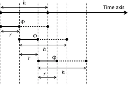
Figure 3.1 shows how the RHA works. The train schedule of t days is divided into three planning horizons of the same size, where each planning horizon only contains train events in the period h. Following the time axis, two consecutive stages start at T and T + r,
Fig. 3.1. Example of RHA illustrations and the notations
respectively, where T is the beginning of the earlier planning horizon. The overlap is the amount of time corresponding to the period (h − r,h). Assume that φ is the end of a roll period, (φ−) is a time attribute less than the end of roll period, and (φ+) is a time attribute greater than the end of roll period. When the whole time horizon is divided into shorter ones, the input of each planning horizon in the RHA needs to contain all information of the corresponding part in original data, in addition to relevant information from the previous period.
3.2. Data & Constraints
In this section, we provide the details of the input given by CN for the LRP with the assumption that the LAP solutions are taken from the railroad or by using the method introduced in Ortiz-Astorquiza et al. (2019). Besides the information used in LRP, we also present how to create the input for the RHA.
Locomotives Data: The basic information of each locomotive contains: ID, type, horsepower, and weight. At the beginning of the week, the locomotives’ status and loca-tion are given. If the locomotive is pulling the train, light traveling or deadheading passing
the beginning of the week, its location is unknown. The locations are determined for lo-comotives grounded in the yards or maintained in the shops. We are also given the set of
critical locomotives due to maintenance in the current week. For each critical locomotive,
we are provided a type of maintenance request determining how long this locomotive will be maintained and the maintenance deadline.
From the second iteration of the RHA to the last one, the information about locomotives’ status and location at the beginning of the planning horizon needs to be taken from the result of the previous iteration. The stations where locomotives are located and locomotives’ status will be updated based on their last activities starting before the end of the roll period (see Section 4.3.4). Furthermore, the critical locomotives can be redefined by comparing their maintenance deadline with the end of the planning horizon. If critical locomotives’ deadlines are greater than the end of the planning horizon, they are changed to “temporary
regular locomotives”, which have no maintenance request. By this change, the railroad not
only avoids maintaining critical locomotives too early before the deadlines but also decreases the number of leased locomotives.
Train Data: The train data contains scheduled trains within a weekly information on each train. For each train in the schedule, we are given basic information such as ID, its departure time and arrival time, its origin and destination station, tonnage, horsepower per tonnage factor. Additionally, we know the set of stations in the route of each train and the distance between each pair of stations. The output of the LAP is also given a set of train-to-train connections that must be satisfied during the week. The train-train-to-train connection is a combination of two trains sharing the same consist and the destination station of the first train is the origin station of the second one. Furthermore, from the result of the LAP, the type and the number of locomotives per type required to pull each train is specified as an input of the operational level.
When implementing the RHA for solving the LRP, we have to extract a part of the
train schedule and train-to-train connections fitting each planning horizon. All trains
departing during the planning horizon and all train-to-train connections containing both trains in this period are taken from the original schedule. The train-to-train connec-tions including the second train out of this period will be considered later (see Section 4.3.1). Station Data: Besides the basic information as ID, name, distance to each other station in the railroad network, each station requires a number of locomotives of each type by the end of the week in order to preserve the power demand at the beginning of the next week.
We are also given a set of stations providing maintenance service. Each station in this subset, called shop, can maintain an exact number, called capacity, of locomotives at the same time. When implementing RHA, the capacity of the shops must be updated at the beginning of each planning horizon based on the data of locomotives. We are also given the set of stations which can connect to each other for light traveling. The locomotives cannot light travel from or to the stations, which are out of this subset.
Cost Data: Several cost parameters used at the LRP are specified by the operational cost data in real-life, such as ownership cost, fuel consumption, track maintenance, locomo-tive crew cost, maintaining cost of critical locomolocomo-tives, and the fixed cost per light travel. The ownership cost presents the weekly spending of owning a locomotive, even if it is not used. The fuel consumption depends on the locomotive type, train fueling consumption rate, and traveling distance. The track maintenance is affected by the locomotive’s weight and the distance it travels. The locomotive crew cost presents human resources spent on operating a locomotive, depending on how long and how far it is traveled by the crew. The maintenance cost is associated with the time required to maintain a critical locomotive, affected by the locomotive’s type. The fixed cost per light travel is added to each light arc not only to perform how expensive when re-positioning a locomotive on that arc but also to distinguish a light travel to a deadhead.
In Miranda et al. (2020), the leasing cost is implicitly being charged on the arcs leased locomotives traverse. Note that in all arcs, the authors charge an ownership cost, which
is the amount to pay for having the locomotive. In the case of a leased locomotive,
the model will own it for the entire planning horizon, so they have to pay the cost of having it from time 0 (i.e., the beginning of the week) to the end of the last operation
assigned to it. When a locomotive flows through some arcs of the graph, a cost that
already includes a small “portion” for owning it during the current planning horizon is
paid. Therefore, even if the authors set the fixed leasing cost to zero, the model tries
to use the least possible number of leased locomotives to save on the ownership cost. In practice, we observe that to reduce the number of leased locomotives in the RHA, the leasing cost should be greater than zero, and its value depends on the length of the planning horizon. Decisions: In Ortiz-Astorquiza et al. (2019), the authors not only consider determining train consists, locomotives repositioning over the network, and train-to-train connections but also take into account the operation mode of each train. The operation mode of a train is defined based on the position of locomotives pulling it. If all locomotives travel together
at the head of a train, the train operates in conventional mode. If locomotives are inter-spersed throughout the length of a train, the train operates under distributed power mode. Additionally, the authors also consider several side-constraints and company’s preferences in order to satisfy the requirement arising in practice.
Based on the result of the LAP, decisions made by the LRP ensure that the different side-constraints and company’s preferences are met. Consequently, they do not need to be considered again at the operational level. For instance, if the result of the LAP decides to operate a train under distributed power, a consist is chosen considering locomotives types that are appropriately equipped to do so. Then, the LRP assigns locomotives units of the selected types to this train in order to satisfy distributed power. To sum up, the sequence of trains each locomotive should operate is determined, while considering locomotive maintenance and a balance flow of locomotives through the space-time network so as to satisfy a given train schedule at a minimum cost.
Objective: The LRP ensures that all scheduled trains and train-to-train connections must be served on time and assigned precisely consists provided by the LAP. Besides, critical locomotives should be maintained as much as possible without exceeding the capacities of shop stations. The problem also aims to minimize the number of deadheads, light travels, and leased locomotives while keeping the network balance. The objective function contains the cost of actively pulling scheduled trains, which is modeled as a function of track maintenance, fueling consumption and ownership costs; the cost of deadheads, which is a function of track maintenance and ownership costs; the cost of light travels, which is considered as a function of track maintenance, ownership, fuel consumption and crew costs; the cost of idling (ownership cost) locomotives at the stations, and the cost of moving critical locomotives through shops, which is calculated as a function of maintenance and the ownership costs.
To use the RHA to solve the LRP, we have to update activities of locomotives when switching from a small planning horizon to the next one. We also deal with all conflicts caused by maintenance requirements and train-to-train connections mentioned in Chapter 4. Constraints: At the operational level, the LRP considers each critical locomotive and groups of regular locomotives to determine their route over the current week. Therefore, the LRP faces both constraints for individual locomotives and the ones for groups of locomotives. Besides minimizing the total of costs mentioned in the previous section, the LRP must satisfy all following constraints:
- Preserving combinations of locomotives in train-to-train connections. - Sending critical locomotives to the shop without exceeding shop capacities.
- Limiting the number of locomotives, both active and deadhead, attached to a train. - Imposing a limit on the distance of each light travel.
- Guaranteeing supply of locomotives at the station at the end of each planning horizon to satisfy the next schedule.
- Obeying the light traveling rule that the locomotives only light travel between a given set of stations.
Chapter 4
Model and Solution Method
In Section 4.1, we present the two-layer space-time network provided by Miranda et al. (2020). The network, which allows us to manage and separate the flow of regular and critical locomotives, is described in Section 4.1.1 and Section 4.1.2. Although the network describes the problem over the short planning horizon, it does not take into account the train-to-train connections wherein two trains do not operate in the same period of time. A new type of arcs is introduced in the Section 4.3.1 in order to solve that issue. The IP model of Miranda et al. (2020) is introduced in Section 4.2, while Section 4.3.2 presents how we modify the IP model when adding new arcs to the network. The RHA framework is implemented in Section 4.3.3. In this section, we study some conflicts arising when dividing the whole planning horizon into smaller ones. Several constraints must be slightly modified to cope with those conflicts. Therefore, a new IP model, which is used in the RHA framework, is presented. Finally, Section 4.3.4 considers the way to update the information of locomotives when switching from a planning horizon to the next one in the RHA.
4.1. The Existing Space-time Network
We describe the two-layer space-time network introduced in Miranda et al. (2020) to describe the physical railroad over time. Let G = {N ,A} be the graph where N is the set of nodes presenting the events at the stations and A is the set of arcs presenting activities of locomotives, such as pulling trains, grounding at the stations, going to the shops for maintenance, deadheading or light traveling. Each node is defined by type (source node, sink node, departure node, arrival node, outpost node), time, and place.
The primary purpose of the two-layer space-time network is to deal with the maintenance operation of critical locomotives. When deciding to send a locomotive to the shop, we must provide a way to maximize locomotive utilization, to meet the maintenance appointment, and to avoid exceeding the shop’s capacity. Because critical locomotives might be attached to a train that takes them far away from shop locations or locomotives have to stand in
line at the shop for a spot, or they have to be sent to other shops with available capacities for being served, CN allows critical locomotives to be maintained after their maintenance deadline. In this situation, the locomotives are called overdue and cannot be used for pulling trains or light traveling requiring locomotives’ power. The overdue locomotives have to wait at the shop until spots are available for them or are sent to other shops by using deadheads. In the graph, they are sent to the top layer to do these actions to separate their flow and the flow of non-overdue locomotives.
While the bottom layer contains all arc types, such as train arcs, train-to-train arcs, deadhead arcs, light travel arcs, shop arcs, and ground arcs, the top layer does not include train arcs, train-to-train arcs, and light travel arcs. Only the critical locomotives that have not missed their deadline and the regular locomotives flow in the bottom layer. An overdue locomotive missing the maintenance appointment will be sent to the top layer right after
finishing the last activity crossing the deadline. In practice, only legacy train arcs are
allowed to pass the critical locomotives’ maintenance deadline in the bottom layer.
4.1.1. Bottom Layer
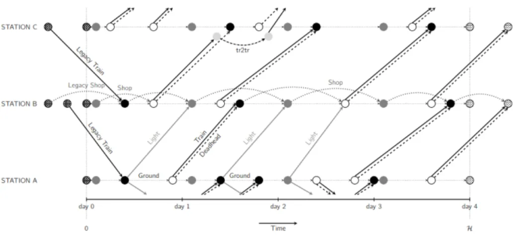
Fig. 4.1. Example of the bottom layer in a space-time network with 3 stations. Source: Miranda et al. (2020)
Figure 4.1 presents an example of the bottom layer in the space-time network with three
stations. Let Nb and Ab be the set of nodes and arcs in the bottom layer. We denote by
Nb
d (white nodes in Figure 4.1), Nab (black nodes in Figure 4.1), Nob (dark grey nodes in
Figure 4.1), Nb
sr (hatched nodes in Figure 4.1), Nsib (dotted nodes in Figure 4.1) the set of
departure nodes, arrival nodes, outpost nodes, source nodes, and sink nodes in the bottom
layer, respectively. A train arc in the set of train arcs Ab
departure node and an arrival node. Each departure node contains the origin station of the train and the time attribute given by the train’s departure time minus the amount of time required to build consist. Similarly, each arrival node represents the train’s destination and the time attribute given by the train’s arrival time plus the time required to bust consist.
At the beginning of the planning horizon, each station is presented by a source node with
a time attribute set to 0. We partition the set Nb
sr into a set of initial nodes Nib acting as
sources of available locomotives at the associated stations and a set of nodes Nb
sr\Nib related
to legacy arcs. Similarly, each station is also represented by a sink node with a time attribute
set to the end of the planning horizon. Let Nb
f and Nsib\Nfb be set of final nodes acting as
the sinks of available locomotives at the end of the planning horizon and the set of nodes associated with actions that cross the end of the planning horizon. In order to ensure that there exists at least one shop or light travel opportunity, outpost nodes are created at each
station at the beginning of each day. From these nodes in the set No = Nob ∪ Not, we can
decide to move locomotives to the shops, or light travel to other stations, or stay grounding. From now on, we assume that nodes at each station are sorted chronologically by their time attribute, and no pair of nodes at the same station has the same time attribute.
The set Ab is partitioned into small subsets: train arcs Ab
t (solid black arcs in Figure 4.1),
train-to-train arcs Ab
t2t (dashdotted arcs in Figure 4.1), deadhead arcs Abdh (dashed arcs in
Figure 4.1), light travel arcs Ab
l (solid gray arcs in Figure 4.1), ground arcs Abg (dotted black
arcs in Figure 4.1), and legacy arcs Ab
leg (solid black arcs for legacy train arcs and dotted
gray arcs for legacy shop arcs in Figure 4.1). As aforementioned, a train arc representing a scheduled train connects a departure node and an arrival node. Along the route of the trains, there exist some intermediate stations where the trains can pick up and release locomotives
on their trips. The deadhead arcs in the set Ab
dh are created to connect the origin stations of
the trains and the intermediate stations, or pairs of intermediate stations, or the intermediate stations to the destinations of the trains. The locomotives traversing deadhead arcs do not provide motive power. For RHA, if deadhead arcs cross the end of the roll period, they will be updated as a legacy train arcs (see Section 4.3.4).
Besides deadhead arcs, using light travel arcs in set Abl is also an effective way of
reposi-tioning locomotives across the railroad. As mentioned in Section 3.2, only a small subset of stations is available for locomotives to light travel among its elements. This is based on the fact that the railroad does not expect locomotives to do light traveling with a long distance. It is an expensive operation consuming track capacity and does not generate any revenue because the locomotives travel by themselves without pulling trains or being attached to railcars. The way to update the status of light travel arcs passing the end of the roll period
is similar to the one used for deadhead arcs. In this thesis, we implement the idea used to generate light arcs, as mentioned in Miranda et al. (2020).
At the tactical level, one of the essential aspects to consider when solving the LAP is train-to-train connections. To deal with that, at the operational level, each train-to-train arc in set Ab
t2t is generated to connect the arrival node corresponding to the first train and
the departure node corresponding to the second train. The flow of locomotives must be preserved along the path: the first train arc - train-to-train arc - the second train arc. From now on, let the first train arc and the second train arc present two trains belonging to a train-to-train connection. Each train-to-train arc is attached a label equal to the index of the second train in this connection in order to distinguish it between the set of all train-to-train arcs.
Shop arcs, Ab
sh, are created based on scheduled maintenance operations for critical
loco-motives. The flow of a critical locomotive on a shop arc presents its visit to a shop, where a specific inspection is carried out. The frequency, length, and cost of maintenance depend on types of a maintenance request, namely, standard, semi − yearly, yearly, and quadrennial. Although the railroad aims to serve critical locomotives before their deadline, they allow serving critical locomotives after their deadlines because of the reason mentioned at the be-ginning of this section. The way to generate the shop arcs is presented in detail in Miranda et al. (2020).
Ground arc, Ab
g, presents locomotives idling at the stations. These locomotives can be
waiting for light travel opportunities, standing in the line for spots in shops, or be available at given stations. We should note that nodes at each station are sorted chronologically by their time attribute. Ground arcs are created between each pair of consecutive nodes, starting from the initial node until the final node is reached.
Finally, we consider the set of legacy arcs Ableg presenting unfinished activities starting
from the previous planning horizon and finishing within the current one. This set is
parti-tioned into Abt− and Absh−. The tails of all legacy arcs are always sink nodes, whose time
attributes are always negative. The head node of a legacy shop arc is set as the first node at the shop station with a time attribute greater than or equal to the end of the inspection.
4.1.2. Top Layer & Connecting Layers
The top layer is built by making a copy of elements of the bottom layer except for train
arcs, train-to-train arcs, and light travel arcs. Let Nt
a, Ndt, Not, Nsrt, and Nsit be sets of
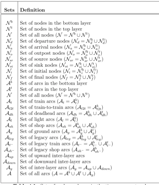
Sets Definition
Nb Set of nodes in the bottom layer
Nt Set of nodes in the top layer
N Set of all nodes (N = Nb∪ Nt)
Nd Set of departure nodes (Nd= Ndb ∪ Ndt)
Na Set of arrival nodes (Na = Nab∪ Nat)
No Set of outpost nodes (No = Nob∪ Not)
Nsr Set of source nodes (Nsr = Nsrb ∪ Nsrt)
Nsi Set of sink nodes (Nsi = Nsib ∪ Nsit)
Ni Set of initial nodes (Ni = Nib∪ Nit)
Nf Set of final nodes (Nf = Nfb∪ Nft)
Ab Set of arcs in the bottom layer
At Set of arcs in the top layer
N Set of all nodes (N = Nb∪ Nt)
At Set of train arcs (At = Abt)
At2t Set of train-to-train arcs (At2t= Abt2t)
Adh Set of deadhead arcs (Adh= Abdh∪ Atdh)
Al Set of light arcs (Al = Abl)
Ash Set of shop arcs (Ash = Absh∪ Atsh)
Ag Set of ground arcs (Ag = Abg∪ Atg)
Aleg Set of legacy arcs (Aleg = Ableg∪ Atleg)
At− Set of legacy train arcs (At− = Ab
t−∪ Att−)
Ash− Set of legacy shop arcs (Ash− = Ab
sh−)
Aup Set of upward inter-layer arcs
Adown Set of downward inter-layer arcs
Ay Set of inter-layer arcs (Ay = Aup∪ Adown)
A Set of all arcs (A = Ab∪ At∪ A
y)
Table 4.1. Sets of nodes and arcs in the time-space network
respectively. Likewise, let Atdh, Atg, Atsh, and Atleg be set of deadhead arcs, ground arcs, shop arcs, and legacy arcs in the top layer.
We also introduce set Ay as the set of the arcs connecting two layers. These arcs, called
inter-layer arcs in Miranda et al. (2020), are used to send the overdue locomotives to the top
layer and return them to the bottom layer for operation after servicing. In the RHA, when there are transitions from planning horizons to others, critical locomotives might be overdue by the end of each roll period. They would be placed on the top layer at the beginning of the upcoming planning horizon. However, it is not essential to make a copy of all legacy arcs in
the bottom layer when building the top one. For example, we can remove legacy shop arcs from the top layer because the locomotives traversing legacy shop arcs can be considered as “nearly” regular ones. By doing this, we do not need to add downward arcs created to move locomotives from the top layer to the bottom layer after finishing their inspections.
In the case of starting and finishing the locomotive’s maintenance within the current planning horizon, we add a downward arc whose tail corresponds to the head of the associated shop arc in the top layer and the head in the bottom layer with identical type, place and time attributes. Conversely, an upward arc is created to connect a tail node in the bottom layer and a head node in the top layer. While the tail of the arc associates with the head node of the last event at the station, the head node is a copy of the tail with the same type, location, and time attribute but in the top layer.
4.2. The Existing Mathematical Formulation
Variables Definition
rkl Number of regular locomotives of type k that traverses arc l
cvl Equals 1 if the critical locomotive v traverses arc l, 0 otherwise
uki Number of leased locomotives of type k supplied by source i
Table 4.2. Decision variables in mathematical formulation
In this section, we provide a mathematical model built upon the space-time network in the previous section. The model introduced in Miranda et al. (2020) is formulated as an IP problem and repeatedly used in the RHA. The model solves the integer multi-commodity flow problem with side constraints to determine which regular and critical locomotives flow on the arcs of the graph. The problem faced by CN considers thousands of locomotives and trains per week. It is hence not possible to consider each locomotive as one commodity of the graph. The regular locomotives are grouped into types similarly in the LAP to decrease the number of variables in the mathematical model, while the critical locomotives are still treated individually. Because of this reduction, the problem is solved to optimality within an acceptable computing time. According to Miranda et al. (2020), it is essential to apply a flow decomposition algorithm introduced by Ahuja et al. (1993) to extract paths for individual regular locomotives while the route of each critical locomotive is presented by the network flow of the commodity associated with it.
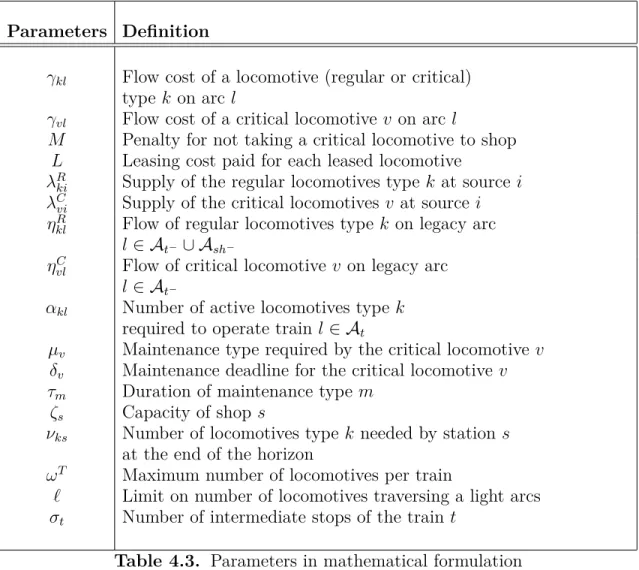
The formulation proposed in Miranda et al. (2020) is presented as follows with all sets, parameters, and variables as summarized in the Tables 4.1-4.4.
Objective function: minX k∈K X l∈At γkl(rkl+ X v∈VC k cvl) + X k∈K X l∈Adh γkl(rkl+ X v∈VC k cvl) + X k∈K X l∈Al γkl(rkl+ X v∈VC k cvl) + X k∈K X l∈Ag γkl(rkl+ X v∈VC k cvl) + X k∈K X l∈At2t γkl(rkl+ X v∈VC k cvl) + X v∈VC X l∈Ash(v) γvlcvl + M X v∈VC (1 − X l∈Ash(v) cvl) + L X k∈K X i∈Nib uki (4.2.1) subject to: rkl= ηklR ∀k ∈ K, ∀l ∈ A b t−∪ Absh− (4.2.2) cvl = ηCvl ∀v ∈ V C , ∀l ∈ At− (4.2.3) X l∈Ok[i] rkl = λRki+ uki ∀k ∈ K, ∀i ∈ Nib (4.2.4) X l∈Ov[i] cvl = λCvi ∀v ∈ VC, ∀i ∈ Ni (4.2.5) X i∈Nb si X l∈Ik[i] rkl = X i∈Nb sr X l∈Ok[i] rkl ∀k ∈ K (4.2.6) X i∈Nsi X l∈Iv[i] cvl = 1 ∀v ∈ VC (4.2.7) X l∈Ik[i] rkl= X l∈Ok[i] rkl ∀k ∈ K, ∀i ∈ Ndb∪ N b a ∪ N b o (4.2.8) X l∈Iv[i] cvl = X l∈Ov[i] cvl ∀v ∈ VC, ∀i ∈ Nd∪ Na∪ No (4.2.9) X l∈Ash(v) cvl ≤ 1 ∀v ∈ VC (4.2.10)