An Iterative Regularized Method for Segmentation with Applications to Statistics

(1)

HAL Id: tel-02473848

https://hal.archives-ouvertes.fr/tel-02473848

Submitted on 11 Feb 2020

HAL is a multi-disciplinary open access archive for the deposit and dissemination of sci-entific research documents, whether they are pub-lished or not. The documents may come from teaching and research institutions in France or abroad, or from public or private research centers.

L’archive ouverte pluridisciplinaire HAL, est destinée au dépôt et à la diffusion de documents scientifiques de niveau recherche, publiés ou non, émanant des établissements d’enseignement et de recherche français ou étrangers, des laboratoires publics ou privés.

Applications to Statistics

Vivien Goepp

To cite this version:

Vivien Goepp. An Iterative Regularized Method for Segmentation with Applications to Statistics. Computation [stat.CO]. Université de Paris / Université Paris Descartes (Paris 5), 2019. English. �tel-02473848�

(2)

Laboratoire MAP5 UMR CNRS 8145

École doctorale 386 : Sciences Mathématiques de Paris Centre

THÈSE

Pour obtenir le grade de DOCTEUR EN MATHÉMATIQUES

Spécialité : Mathématiques appliquées

Présentée par

V

IVIEN

G

OEPP

A

N ITERATIVE REGULARIZED METHOD FOR

SEGMENTATION WITH APPLICATIONS TO STATISTICS

Sous la direction d’OLIVIERBOUAZIZet GRÉGORYNUEL.

Soutenue publiquement le 27 septembre 2019 devant un jury composé de

Olivier BOUAZIZ Université Paris Descartes Directeur de thèse

Julien CHIQUET Agro ParisTech Rapporteur

Chantal GUIHENNEUC Université Paris Descartes Examinatrice Hélène JACQMIN-GADAA Université de Bordeaux Présidente du jury Catherine LEGRAND Université Catholique de Louvain Rapporteure

Grégory NUEL Sorbonne Université Directeur de thèse

Jean-Christophe THALABARD Université Paris-Descartes Examinateur

(3)

(4)

This thesis deals with the development of regularized methods using penalized maximum likelihood estimation. More specifically, I use a sparsity-inducing iterative method called adaptive ridge. The latter is competitive compared to other approaches, namely in terms of ease of implementation and computational cost. My work consists in the application of this method to a wide range of problems: survival analysis, spline regression, and spatial segmentation. Applications in several problematics show that the adaptive ridge’s good performance in selection, great ease of implementation and low computational cost can make it a good starting point in penalization-base variable selection.

In survival analysis, data are often collected by following a cohort, in which case the events are widely spread through time and the sample is suspected to present heterogeneity. I first focus on developing a method for the inference of the incidence, which allows to detect heterogeneity with respect to the date of birth (or cohort). A closely related problem is the study of the evolution of the inference as a joint function of the age, the date of birth (cohort), and the calendar time (period). Epidemiologists have long resorted to the age-period-cohort model or its submodels. The latter as-sume linear effects of each variable, which is deemed too simplistic to estimate potentially important features of the incidence. In this framework, I develop a model allowing for the joint estimation of two variables’ effects and of their interaction.

Spline regression is known to be a competitive method for non-parametric regression. However the estimated spline depends highly on the initial choice of knots and choosing the best knots is a computationally hard problem. I propose an approach for the estimation of the best knots jointly with the spline function. By initiating a large number of knots and successively removing the least relevant ones, my method makes a slightly restrictive hypothesis to remove much of the computa-tional burden.

In spatial statistics, the spatial domain is often divided into “units” and data are gathered at the unit level. The spatial effect is estimated on each unit and its representation is subject to the arbitrary of the unit division, which makes its interpretation difficult. This can be resolved by regularization, which reduces the variance and increases the interpretability. I present a model for segmentation of spatial data based on the adjacency structure of the units.

(5)

(6)

Cette thèse porte sur l’élaboration de méthodes régularisées utilisant l’estimation par maximum de vraisemblance pénalisée. Plus précisément, j’utilise une méthode parsimonieuse itérative, appelée adaptive ridge. Cette dernière est compétitive par rapport à d’autres approches, notamment en ter-mes de facilité de mise en œuvre et de temps de calcul. Mon travail consiste à appliquer cette méth-ode à un large éventail de problèmes : l’analyse de survie, la régression par splines et la segmentation spatiale. Ces applications dans différentes problématiques montrent que la bonne performance de l’adaptive ridge en sélection, sa grande facilité de mise en œuvre et son faible coût de calcul peuvent en faire un bon point de départ dans les méthodes de sélection de variable par pénalisation.

En analyse de la survie, les données sont souvent recueillies en suivant une cohorte, auquel cas les événements sont largement répartis dans le temps et l’échantillon peut présenter une hétérogénéité. Je me concentre d’abord sur le développement d’une méthode d’estimation de l’incidence qui per-met de détecter l’hétérogénéité par rapport à la date de naissance (ou cohorte). Un problème proche est l’étude de l’évolution de l’inférence en fonction de l’âge, de la date de naissance (cohort) et de la date calendaire (period). Les épidémiologistes ont longtemps eu recours au modèle age-period-cohort ou à ses sous-modèles. Ces dernières supposent des effets linéaires de chaque variable, ce qui est jugé trop simpliste pour estimer des caractéristiques potentiellement importantes de l’incidence. Dans ce cadre, j’élabore un modèle estimant cojointement l’effet de deux variables et de leur inter-action.

La régression par splines est connue pour être une méthode performante de régression non paramétrique. Cependant, la spline estimée dépend fortement du choix initial des nœuds et le choix des meilleurs nœuds est un problème difficile en pratique. Je propose une approche perme-ttant l’estimation des meilleurs nœuds conjointement avec la fonction spline. En initiant un grand nombre de nœuds et en supprimant successivement les moins pertinents, ma méthode fait une hy-pothèse légèrement restrictive pour diminuer grandement le temps de calcul.

En statistiques spatiales, le domaine spatial est souvent divisé en "unités" et les données sont recueillies au niveau des unités. L’effet spatial est estimé sur chaque unité et sa représentation est soumise à l’arbitraire de la division de l’unité, ce qui rend son interprétation difficile. Ceci peut être résolu par la régularisation, ce qui réduit la variance et augmente l’interprétabilité. Je présente un modèle de segmentation des données spatiales basé sur la structure d’adjacence des unités.

(7)

(8)

Plan of this thesis

This thesis is organized as follows:

Chapter 1 introduces, compares, and discusses the main statistical approaches to model selection.

A great emphasis is laid on penalized likelihood methods. First, I detail the most famous methods of penalized maximum likelihood estimate: the lasso, the elastic-net, and further refinements. I de-velop on the use of these penalties in the linear model. Secondly, I touch on two of the methods of model selection which are not based on penalization: best subset selection and stepwise selection. In the third section, I introduce the Majorize-Minimization (MM) optimization scheme, which, applied to penalized likelihoods, yields two important iterative penalized methods: the Local Linear Approx-imation (also termed adaptive lasso) and the Local Quadratic ApproxApprox-imation. I then introduce the iteratively defined penalized method used throughout this work: the adaptive ridge. Finally, I de-velop on the statistical methods which enforce an a priori structure on a parameter.

Chapter 2 deals with the application of the adaptive ridge to the context of hazard estimation in

survival analysis. After an introduction on the topic, and an illustration of the method to a one-dimensional case, we detail how the fused adaptive ridge allows for a new method of regularized es-timation of the bi-dimensional hazard rate, with detection of breakpoints. Even though this methods applies to a wide array of problems, we illustrate it through the angle of age-period-cohort analysis.

Chapter 3 deals with the same problem than Chapter 1, but through the context age-period-cohort

analysis. We first introduce the topic of age-period-cohort analysis, as well as the use and drawbacks of the age-period-cohort model. Then, we develop on the “Age-Cohort-Interaction ” model, which builds on the works of the previous chapter. This model can be viewed as a generalization of the age-period-cohort analysis, which does not suffer from its defects, at the added cost of computation time.

Chapter 4 deals with a different application of the adaptive ridge. In this part, we apply this method

to the problem of finding the best knots to support a regression spline. This problem has long been deemed computationally intractable. We show that provided some simplifying assumptions, our new spline regression method can select the best knots as well as the regression spline in a fast fashion. Before developing on our method, we introduce the topic of spline regression and present the main tools and issues in this topic.

Chapter 5 deals with the applications of the adaptive ridge to regularization of spatially-correlated

data. When the statistical problem has a spatial structure that is given in already chosen zones, the problem of regularization becomes challenging. We introduce a method for regularization along a graph, with an application to inference for medical data.

The works of Chapters 2 and 4 has lead to two preprints currently under revision. These two chapters consist of these preprints, reproduced as is and preceded by introductory talks on their respective matters. These two papers are given in Sections 2.2 ad 4.2, with respective supplementary materials given in Sections 2.3 and 4.3 respectively. These papers define their own notations, which

(9)

are for the most part consistent with the rest of the manuscript. Except for these sections, the present document forms a consistent manuscript, even if the Chapters were divided so as to be able to be read separately.

(10)

Scientific communications

Scientific papers

• Bidimensional estimation of the hazard rate [Submitted]1 • Age-Cohort-Interaction model [In progress]

• Spline regression [Submitted]2 • Spatial regularization [In progress]

Conferences

Contributed Talks

• L0 Regularization for the estimation of piecewise constant hazard, SAM Conference 2017. • Regularized Hazard Estimation for age-period-cohort Analysis, International Workshop on

Ap-plied Probability 2018.

• Estimating interactions effects in the age-cohort model, Research group “Statistiques et santé”

2018.

Seminars

• Some applications of the adaptive ridge to survival analysis, Meeting of the LPSM Biology Group, April 2019.

• Estimation régularisée du risque pour l’analyse age-period-cohort, MAP5 Seminar of Statistics, 2017.

• Heterogeneity in Survival Analysis, Rencontre des Jeunes Statisticiens, 2019.

Posters

• Regularized Hazard Estimation for age-period-cohort analysis, Statistical Methods for

Post-Genomic Data 2018.

• Regularized Hazard Estimation for age-period-cohort Analysis, International Biometric

Con-ference 2018.

• Interaction Effects in Age-Period-Cohort Analysis, Statistical Methods for Post-Genomic Data

2019.

1_{https://hal.archives-ouvertes.fr/hal-01662197v3} 2_{https://hal.archives-ouvertes.fr/hal-01853459}

(11)

Software

• Packagehazreg, available on github3. • Packageaspline, available on github4. • Packagegraphseg, available on github5.

3_{https://github.com/goepp/hazreg} 4_{https://github.com/goepp/aspline} 5_{https://github.com/goepp/graphseg}

(12)

Notations and Definitions

Definitions

• The Lq norm of a vector u is noted kukq. The L2norm is also abbreviated kuk.

• E [X ] and V[X ] denote the respective expectation and variance of the random variable X . • Tr denotes the trace.

• →ddenotes the convergence in distribution.

• AT denotes the transpose of the matrix A.

• min+{u} denotes the minimum taken only over the positive values of the vector u • (x)₊denotes the positive part of x, that is max (x, 0).

• diag{ui}iis the diagonal matrix whose non-zero entries are u1, . . . , un.

• N (.,.) denotes the (possibly multivariate) normal distribution. The two arguments are the expectancy and variance.

• #A denotes the cardinal of the set A.

• When f is a function and x an element from its domain, f (x−) and f ¡x+_{¢ denote the}

lim-its lim_{t →x}f (t ) in the cases t < x and t > x, respectively.

Notations

• Vectors and matrices are noted in bold. When necessary, vectors are identified with column matrices.

• n is the sample size

• i ∈ {1,...,n} is the index of the individuals • p is the number of covariates

• j ∈©1,..., pª is the index of the covariates

• In the context of penalized likelihood methods,λ ∈ R is the penalty constant; in the context of survival analysisλ : R 7→ R+is the hazard rate.

• β is the parameter to be estimated

• I refers to the identity matrix, whose dimension depend on the context. • ` = −logL is the negative log-likelihood and L is the likelihood.

• I use the symbol “,” when the equality serves as a definition. ix

(13)

Abbreviations

• MM: Majorize-Minimization optimization • NLL: negative log-likelihood

• LQA: Local Quadratic Approximation • LLA: Local Linear Approximation • AIC: Akaike Information Criterion • BIC: Bayesian Information Criterion • OLS: Ordinary Least Squares (estimate) • MLE: Maximum Likelihood Estimate • PCH: Piecewise Constant Hazard (model) • LARS: Least Angle Regression

Conflicts in notation between chapters

We have tried to use coherent and non-conflicting notations for the mathematical objects defined in this thesis. However, for the sake of consistency with the conventions of the field, we made the choice to keep conventional notations for known quantities. The instantaneous hazard rate for instance, is notedλ(t) (as a function of t) as is standard in survival analysis and in the study of stochastic pro-cesses. In other parts of the manuscript, we also used the variableλ to denote the penalty constant in penalized maximum likelihood methods.

These notational conflicts have been kept to ease the understanding of the manuscript. They occur between different chapters but not inside each chapter. We stress that the potential uncertainty is removed when the context is taken into consideration.

(14)

Introduction

This thesis deals with the application of penalized methods to different statistical problems. These works all have in common the use of a penalized maximum likelihood method– called the “adaptive ridge” – which performs model selection. The latter comes from a long line of historically, practically, and theoretically important regularization methods, which date back to the very beginning of com-putational statistics. These methods are at the intersection of different fields: statistics, optimization, and computer science.

It is therefore necessary to introduce the most important of these methods in order to (i) highlight the principle of penalized estimation methods, (ii) put the adaptive ridge in the context of the other model selection methods, and (iii) compare the adaptive ridge with the competing methods. This introduction serves this purpose.

Variable selection methods have been developed since the 1970’s, with the use of the stepwise selection and the ridge regression in the context of linear regression. But their use and fame have exploded only in the 1990’s and early 2000’s, with the development of penalized regression method, and in the first place of the lasso, introduced in the field of statistics by Tibshirani (1996) and in signal processing by Chen et al. (2001) under the name “basis pursuit”. These methods have been introduced for linear regression, but their principle applies to any statistical model whose likelihood is computable and practical to maximize. Penalized regression methods consist in adding a term in the negative log-likelihood (NLL) to minimize. This term enforces the estimate to be close to an a

priori shape or distribution. Certain penalty terms have been found to induce the desired properties

of the estimate: the resulting estimate is both better quantitatively, i.e. it has better estimation per-formance, and qualitatively, i.e. it infers models which are more relevant and easier to interpret, than standard estimates. These methods sparked a revolution in the field of computational statistics: the added penalty term increases the complexity of the computation by a low margin and the benefits are huge in many practical applications.

A whole array of these penalized methods have then been developed and improved upon, with penalties ever more refined and adapted to the problem at hand. However, the initial application of penalized estimation with variable selection is the linear model, and its extension to non-Gaussian errors, the generalized linear model. It seemed that in this case, the goal to find easy- and fast-to-compute methods that are performant both theoretically and practically, has been met. Two other major fields of applications of penalized methods have emerged around this period: high throughput data and wavelet analysis. The former became widely popular in the last decade due to the onset of next-generation sequencing technologies. Since many genes are studied at once, we are in a case where p À n, usually by a factor ∼ 100. The problem posed by this high-dimensional setting was seldom met in usual regression settings, and led to the development of penalized regression methods for what is called high-dimensional statistics. The latter comes from the development of wavelets bases and their applications to all fields of signal processing. Wavelets are families of functions that form an orthogonal family of L2(R), are located in both the time and frequency domains, and are all the scaled and shifted versions of one another. These properties make it the tool of choice for

(19)

representing signals (i.e. audio signals, images, videos, etc.) efficiently. Indeed, the wavelet bases allow for sparse representation of signals, with major applications to denoising, compression, and compressed sensing. In these problems, the signal sparsity is enforced using a penalized approach. This has sparked the development of penalized likelihood approaches that are specifically fit to the topology of the signal. Note that the leap forward made in that domain around the year 2010 was also enabled by the progress in convex optimization (Boyd and Vandenberghe, 2004). We refer to Mallat (2009) for more details on the wavelet analysis and to Bach (2011) for more details on the application of penalized methods to wavelet analysis.

This introduction is organized as follows. The first part draws a panorama of the main penal-ized methods for model selection, with comparisons, explanations, and insights. The second part deals with subset selection, the main model selection method that does not used a penalized ap-proach. The third part puts the iterative penalized methods in the theoretical framework of Majorize-Minimization (MM) optimization and compares the main iterative penalized methods amongst which is the adaptive ridge. The last section presents modifications of the penalty terms which enforces the estimate to have a certain sparsity structure, which is more general than being sparse. We arrive at the fused adaptive ridge, which is used in Chapters 2 and 3.

(20)

Contents 1.1 Regularized estimation . . . . 4 1.1.1 Ridge regression . . . 5 1.1.2 Lasso estimation . . . 7 1.1.3 Elastic-net . . . 12 1.1.4 Bridge regression . . . 12 1.1.5 Berhu . . . 13

1.1.6 Penalized likelihood methods as a Bayesian prior . . . 13

1.1.7 Non-concave penalties . . . 15 1.1.7.1 Hard-thresholding . . . 17 1.1.7.2 SCAD . . . 18 1.1.7.3 Logarithmic penalty . . . 18 1.1.7.4 Available implementations . . . 19 1.2 Subset selection . . . 19

1.2.1 Best subset selection . . . 19

1.2.2 Stepwise Selection . . . 20

1.3 Iterative penalized methods . . . 21

1.3.1 MM optimization . . . 21

1.3.2 MM optimization applied to non-concave penalties . . . 22

1.3.2.1 Local Quadratic Approximation . . . 23

1.3.2.2 Local Linear Approximation . . . 24

1.3.3 Adaptive Ridge . . . 25

1.3.3.1 Relation to similar procedures . . . 27

1.3.3.2 Numerical performance . . . 28

1.4 Structured variable selection . . . 28

1.4.1 Group lasso . . . 28

1.4.2 Overlapping groups . . . 30

1.4.3 Hierarchical structured sparsity . . . 31

1.4.4 Fused lasso and total variation . . . 32

1.4.5 Fused Adaptive Ridge . . . 34

(21)

1.1 Regularized estimation

Linear regression. Consider the linear regression setting

y = X β + ε, (1.1)

where y is the n × 1-sized response variable, X =¡xi , j¢ is the n × p-sized design matrix, β is the p × 1

parameter vector of linear effects, andε is the p × 1 vector of random errors. The columns of X are called the covariates and are noted xj. We consider the case of deterministic design, that is, X is

deterministic.

Linear regression is sometimes written

ˆy = ˆβ0+ X1βˆ1+ · · · + Xpβˆp,

which includes the estimation of an interceptβ0, adding a row of 1s in the design matrix X . Since

the maximum likelihood estimate ofβ0is ¯y =_n1Pn_{i =1}yi, we will instead consider the model (1.1) and

always assume that the response variable is centered: ¯y = 0.

It is also necessary that the covariates be scaled, both for the numerical stability of the computa-tions and to be able to compare the effects of each covariate. For instance if the unit of xjis changed

from meters to millimeters, ˆβjis multiplied by 1000. Hence the effect of that covariate will be

artifi-cially inflated and it will always be selected by a model selection method. Thus, the covariates have to be scaled for their effects to be comparable. Note that there is an equivalence between fitting the parameters on the unscaled covariates and fitting them on the scaled covariates and applying the corresponding scaling to each parameter. Therefore, without loss of generality, we will assume that

n X i =1 xi j= 0 and n X i =1 x2_{i j}= 1, 1 ≤ j ≤ p.

The ordinary least squares (OLS) is

ˆ

βols,arg min

β ky − X βk

2

2=¡XTX

¢−1

XTy. (1.2)

If not stated otherwise, we assume the two classical following assumptions to hold.

Assumption 1. yi= xiβ∗+εi, whereεiare independent and identically distributed random variables

of mean 0 and varianceσ2, andβ∗ is the real value ofβ that we estimate. Note that unless stated otherwise, the errors are not assumed to be normally distributed.

Assumption 2. The matrix_n1XTX → C , where C is positive definite.

Penalized likelihood. In the forthcoming sections we will discuss penalized regression methods, in

which the estimator is defined as the minimizer of the least squares residuals with an added penalty term. In the linear model, when the residuals are normally distributed, the least squares residuals °

°y − X β

° °

2

2 is (proportional to) the negative log-likelihood`¡β¢ of the model. The regularization –

and variable selection – methods present in this introduction have been developed in the setting of linear regression, with the case of normal residuals as an important specific case. In all generality, they can apply to any parametric model that we want to regularize. In this introduction, the notation

`¡β¢ refers to the negative log-likelihood in the linear model or in any unspecified parametric model.

In applications and illustrations however, we will mostly use the linear model to illustrate the effect of penalized estimation.

(22)

• Robust regression, in which the negative log-likelihood writes

`¡β¢ =Xn

i =1

ρ(yi− xiβ) (1.3)

whereρ is a function giving little importance to large values of the residuals. For instance, whenρ(x) = |x|, the model becomes the least absolute deviation, a robust alternative to the linear regression. When ρ is a ρ-function (as defined in Huber et al., 1964), the model is a robust version of the linear model. See Maronna et al. (2006) for a thorough explanation of robust regression.

• The generalized linear model the response variable has a distribution in the exponential family, where the density of y_i (in its canonical form, see McCullagh, 1984, Section 2.2.2) writes

f (y) = exp¡

θ∗

iT (y) − A(θ∗i)) + B(y)¢ ,

where A and B are known deterministic functions andθ_i∗is the true unknown parameter to be estimated. In the generalized linear model, we estimate the density’s parameter vectorθ∗by a function of the linear effect xiβ, and we have E [Y ] = g−1¡Xβ¢ where g is a link function.

Usu-ally we take the canonical link function given by the distribution of y : g−1= A. The negative log-likelihood (nll) writes

`¡β¢ = −Xn

i =1

log f¡g ¡xiβ¢, yi¢ , (1.4)

where f is the distribution of y . For example, if y is Poisson distributed, the canonical link function is the log function and the nll writes

− n X i =1 © yixiβ − exp(xiβ) − log(yi!)ª . 1.1.1 Ridge regression

The OLS estimate is unbiased and has minimal variance amongst all unbiased estimates. However, when the covariates xj are highly correlated, XTX becomes close to singular, i.e. when its largest

eigenvalue gets close to zero, the variance of the OLS diverges to infinity. In this case, a biased modi-fication of the OLS estimate is necessary to control the variance of the estimate. The ridge regression, defined below, is the most famous of such modifications – owing first to its simplicity. It was intro-duced in the context of linear regression and we use this specific case to illustrate its principle and effect, but it extends naturally to any other model. It is obtained by adding a regularizing term to the nll, in the way defined below.

Hoerl and Kennard (1970) introduced the ridge estimator. It is defined as the solution to min

β ky − X βk

2

2+ λkβk22, (1.5)

whereλ > 0 is a trade-off hyper-parameter to be chosen. Problem (1.5) has the explicit solution

ˆ

βridge=¡XTX + λI¢−1

XTy. (1.6)

Equation 1.6 can be seen as a relaxation of the matrix XTX . When the covariates are too

corre-lated, the columns of X are close to being linearly dependent, and XTX tends to be singular.

Equiv-alently, this means that the lowest eigenvalue of XTX tends to zero. Ifλ1is the lowest eigenvalue

of XTX , the lowest eigenvalue of XTX + λI is λ1+ λ. Equation 1.6 can be seen as a modification of

(23)

● β ^ols ● β ^ridge IIy−XβII2 −1 0 1 2 −1 0 1 2 β1 β2

Figure 1.1: Visualization of the ridge estimate as the projection of the OLS onto an L2norm ball. The

ellipses are level curves of the quadratic form ky −X βk2₂. The projection onto the circle of radius t = 1 has the effect of shrinking the estimate’s coordinates together.

Projection on an L2ball. Problem (1.5) is the Lagrangian dual of the problem

min

β ky − X βk

2

2 s.t. kβk22≤ t (1.7)

for t > 0. The two problems have been shown (Boyd and Vandenberghe, 2004, B.1) to have strong duality, that is, for everyλ > 0, there exists a t > 0 such that the solution of (1.7) is also the solution of (1.5), and conversely. The decreasing one-to-one relation betweenλ and t depends on the data.

The equivalent constrained optimization problem helps understand the effect of the penalty in-cluded in ridge regression. Figure 1.1 illustrates the shrinkage of ˆβ due to the projection onto the L2

norm ball. We recall that in a normed vector space, for a chosen norm, the ball of radius r > 0 and of center c is the set of elements at a distance r or less to c, i.e. the set {x|kx −ck ≤ r }. In this manuscript, we will only consider centered balls, that is, balls of center 0. Balls of radius 1 are called unit balls.

Ridge regression in orthogonal design. Consider the case of orthogonal design, that is, when the

design matrix is orthogonal: XTX = I . Notice that in this case, the quadratic terms ky − X βk2=

yTy − 2yTXβ + βTβ and kXTy − βk2= yTX XTy − 2yTXβ + βTβ differ only by a constant. Then the

linear regression boils down to minimizing kz − βk2, where z = XTy is the transformed data. The

ridge problem (1.5) rewrites

min

β kz − βk

2

+ λkβk.

This particular case is important because it is the case in which the covariates are uncorrelated, and the estimation is done component by component. Also, the last equation can be interpreted as find-ing the closest vector to the data z with a small L2norm. This result can also be seen directly through

the simplifications in (1.2) and (1.6).

In this case, then, we have ˆβols= XTy and

ˆ

βridge= ˆ

βols

1 + λ.

Consequently, in orthogonal design, the ridge estimate simply shrinks every coordinate of the OLS towards 0 by the same factor.

Minimization of the MSE. Define the mean square error as

MSEols= E

h

k ˆβols− β∗k22

(24)

Defineλ1≥ · · · ≥ λp > 0 as the eigenvalues of XTX . Recall that the OLS is unbiased and from the

equality ˆβols− β∗= (XTX )−1_XT_{ε, we obtain}

MSEols= σ2Tr{¡XTX¢−1} = σ2 p X i =1 1 λi . (1.8)

This MSE takes problematically large values whenλ1is small.

The ridge estimate aims at reducing the MSE to a value lower than (1.8). The ridge estimate reduces the variance of the estimate, at the price of an non-zero bias. More precisely, the MSE of the ridge estimate decomposes as follows. Consider the singular value decomposition of X :

X = U DVT, (1.9)

where U and V are n ×p and p ×p orthogonal matrices respectively, such that UTU = VTV = Ip, and

D is a diagonal matrix whose entries d1≥ · · · ≥ dp≥ 0 are the singular values of X . From the equality

XTX = V D2VT, we can see that the d2_js are the eigenvalues of XTX . By plugging (1.9) into (1.6), we

get MSE(λ) = E[k ˆβ − β∗k2] = λ2β∗T(XTX )−2β∗+ E£ εX (XT X + λI )−2XTε¤ = λ2β∗TV D−4VTβ∗+ σ2 p X j =1 d2_j (d2_j+ λ)2. (1.10)

In the last equation, the first term is the bias of the ridge estimate, the second term is its variance. Since d MSE dλ (λ) ¯ ¯ ¯ ¯_λ=0₊< 0,

there exists a value ofλ such that the ridge estimate has a smaller MSE than the OLS. 1.1.2 Lasso estimation

Why select variables. In many practical situations, the statistician does not know what covariates

has an influence on the response variable or does not want to make such an assumption a priori. A solution is to add all possible variables and find a regression procedure which simultaneously selects the relevant covariates and estimates their effect. This is the framework of regression with variable selection.

Lasso as a relaxation of the L0norm. Define the L0“norm” kxk0= #{i |xi6= 0} as the number of

non-zero elements of a vector. This quantity is not a norm, because forα 6= 0, kαxk06= |α|kxk. We still

refer to it as a norm since it can be seen as the limit of the Lq norm when q → 0.

The L0penalized likelihood approach offers to minimize

ky − X βk22+ λkβk0. (1.11)

The minimizer of (1.11) represents a trade-off : it has both to be close to the minimum of the squared residuals and to have few non-zero coordinates. Consequently this estimate will only select the most relevant covariates in the model and estimate their effect.

Unfortunately, to minimize the L0norm is NP-hard (Natarajan, 1995), which implies that there is

no known algorithm that can solve an L0norm-constrained problem in a polynomial time complexity

with respect to p. Consequently, this problem has to be solved by trying all the possibilities, which has exponential time complexity in p. This is unfeasible in practice for p ' 50 or larger.

(25)

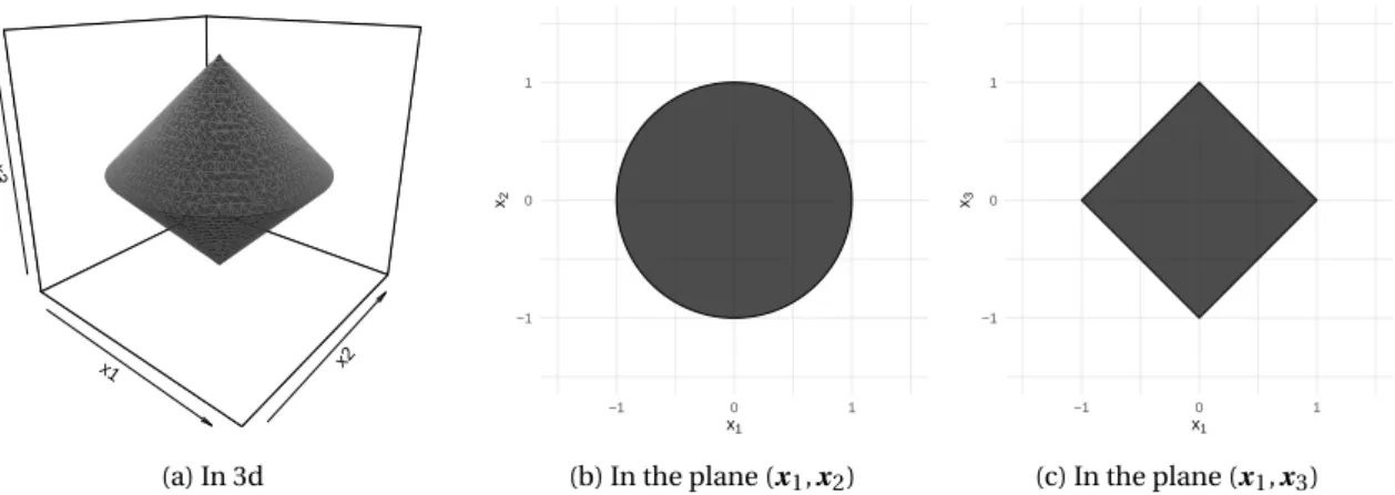
−1.0 −0.5 0.0 0.5 1.0 −1.0 −0.5 0.0 0.5 1.0 β1 β2 Lq Norms q=0.5 q=1 q=2

Figure 1.2: Illustration of Lqunit balls for different values of q.

Tibshirani (1996) introduced the lasso estimator defined by ˆ

βlasso,arg min

β ky − X βk

2

2+ λkβk1 (1.12)

whereλ > 0 is a hyper-parameter which tunes the trade-off between goodness of fit and regulariza-tion. The choice ofλ is not touched on in this chapter. Lasso uses the L1norm which can be seen as

a relaxation of the L0norm.

The L1norm has been used for many decades to recover sparse vectors. In signal processing, a

signal y is expressed as a combination of functions forming a dictionaryφ. Since φ is over-complete, it has more columns than rows, and the coefficient vector x of the decomposition of the signal in the dictionary is not uniquely determined by the problem y = φx. However one assumes that y has a sparse representation in the dictionary. By enforcing a sparsity constraint over x, a compressed representation of the signal y is obtained. Using the L1penalized problem to recover a signal is called

basis pursuit. This method was developed by Chen et al. (2001); it was further analyzed by Donoho

and Huo (2001) and Elad and Bruckstein (2001).

Using the Lagrange multipliers, the lasso estimator can be defined as the projection of the OLS onto the L1ball of radius t :

ˆ

βlasso= arg min

β ky − X βk

2

2 s.t. kβk1≤ t , (1.13)

where t > 0 has a decreasing one-to-one relation with λ. Figure 1.2, which represents Lq unit balls

for different values of q, illustrates why the L1 norm induces sparsity. When q > 1, the Lq ball is

smooth and the projection onto the ball does not set any coordinate to zero. When q ≤ 1, the Lq

ball has singularities at the axes and the projection onto the ball can set some coordinates to zero. Moreover for q ≥ 1, Lq norms are convex, which makes computational minimization way easier. The

L1norm naturally comes out as the only easily minimizable penalty which enables variable selection,

amongst all Lq norm penalties.

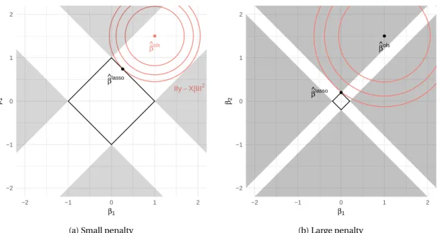
L1norm and sparsity. As previously explained, the projection onto an L1ball can set some

coordi-nates to zero. This phenomenon is illustrated in Figure 1.3 with p = 2. The grey areas represent the half-cones from which a projection on the L1ball sets one coordinate to zero. Consequently, when

ˆ

βolshas a coordinate of small value, its projection maps it to zero. The lasso has the effect of select-ing the covariates with a non-negligible effect on y . As illustrated in the figure, asλ increases the

(26)

● β ^ols ● β ^lasso IIy−XβII2 −2 −1 0 1 2 −2 −1 0 1 2 β1 β2

(a) Small penalty

● β ^ols ● β^lasso −2 −1 0 1 2 −2 −1 0 1 2 β1 β2 (b) Large penalty

Figure 1.3: Illustration of the lasso estimation under orthogonal design. Projection onto two L1norm

balls of radius t . As t decreases, the OLS will most probably end up in a greyed area and the lasso estimate will become sparse.

radius of the ball decreases and the grey area takes up a larger proportion of the parameter space. Consequently, the lasso will tend to set many covariates to zero as the penalty increases.

Lasso in orthogonal design: the soft-thresholding operator. In orthogonal design (see previous

Section), the lasso problem reduces to the component-wise problem ˆβlasso_j = arg minβjf (βj) where

f (βj) =1₂( ˆβols_j − βj)2+ λ|βj| and where ˆβ

ols

= XTy is the OLS estimate in orthogonal design. Since f

is the sum of two functions, who minima are in ˆβols_j and 0 respectively, its minimum is located either at 0 or atβols_j . By considering the two cases |βols_j | ≤ λ and |βols_j | ≤ λ separately, we get that the lasso solution has the explicit solution given by

ˆ

βlasso= S( ˆβols),sgn( ˆβols)³¯¯ ¯βˆ ols¯ ¯ ¯ − λ ´ +, (1.14)

where the function S is called the soft-thresholding function, and where the latter formula is to be considered component by component. This function is equal to zero over the interval [−λ,λ], which means that in orthogonal design, the lasso sets small value of the data to zero.

We refer to Section 1.1.7 for a graphical representation of the soft-thresholding operator and a discussion of its properties.

Computation of the lasso solution. Nevertheless, since the L1norm is not differentiable at the

min-imum, the computation of the lasso estimation is not straightforward. Two algorithms for solving the lasso have gained popularity since its development.

The Least Angle Regression (LARS) algorithm has been proposed by Efron et al. (2004) and offers to compute the whole regularization path1. It initiates with no covariates in the model and sequen-tially adds the covariate that has the maximum correlation with the residuals. The estimate is in-creased linearly in the direction of equal correlation between all active covariates (hence the names

1_{The regularization path of a regularized model is the path of solutions ˆ}_{β(λ) represented as a function of λ. This path}

(27)

least angle). Once a new covariate has the same correlation with the residuals as the current

covari-ate, it is added to the set of active covariates and becomes the current covariate. This method is explained in more details in the Appendix.

Another approach is the coordinate descent, a simple optimization method that is particularly fit to solving the lasso. This method is explained here.

The coordinate descent was initially proposed for the lasso by Fu (1998) under the name of

shoot-ing algorithm. It was generalized to other related penalties by Friedman et al. (2007). The method

solves the lasso problem for a fixedλ.

The algorithm starts with an initial guess ˆβ(0)and minimizes the penalized residuals with respect to each component in a fixed cyclical order until convergence. For 1 ≤ k ≤ p, we denote by βk the

k-th component ofβ. The minimization of (1.12) with respect to βk writes

min βk n X i =1 ³ ˜ y_i(k)− xi ,kβk ´2 + λ|βk| (1.15)

where ˜y_i(k),yi−P_{j 6=k}xi jβj. The solution to this problem is simply the soft-thresholding operator

applied to the modified output:

β∗ k= Ã¯ ¯ ¯ ¯ ¯ n X i =1 ˜ y_i(k)xi k ¯ ¯ ¯ ¯ ¯ − λ ! + sgn Ã _n X i =1 ˜ y(k)_i xi k ! (1.16)

Hence the coordinate descent algorithm for the lasso is simple, easy to implement and fast to com-pute. However, contrarily to LARS, it does not compute the solution path for all penalties; we fix a grid of penalties and compute the coordinate descent for each penalty. To speed up the computation, the initial value in the coordinate descent is taken as the minimum found for the previous penalty. This computational trick is often referred to as warm start. The coordinate descent procedure with one penalty is given in Algorithm 1.

Algorithm 1 Coordinate descent with one penalty 1: function COORDINATE-DESCENT(y , X ,λ)

2: β ← ¡Xˆ TX¢−1

X y

3: k ← 1

4: while not converge do 5: y˜_i(k)← yi−P_{j 6=k}xi jβˆj 6: βˆk← S ³ Pn i =1y˜ (k) i xi k,λ ´ 7: k ←¡k mod p¢ + 1 8: end while 9: end function

In the lasso regression, the function to minimize is the sum of the residuals, which is convex differentiable, and the L1norm, which writes as the sum of univariate convex functions. The rational

behind the use of coordinate descent to solve the lasso problem is the following property.

Property 1. Consider a function f :Rp→ R which writes f ¡

β¢ = g ¡β¢+Pp_{j =1}hj¡βj¢ where g is convex

differentiable and the hi, 1 ≤ i ≤ p are convex. Assume that β∗is a minimum of f along all coordinates,

that is: ∀i ∈©1,..., pª,∀a ∈ R, f ¡β∗_{+ ae}

i¢ ≥ f ¡β∗¢ where ej is the jt hbasis vector. Thenβ∗is a global

minimum.

Proof. Letβ∗be a minimum of f along all coordinates. For anyβ:

f¡ β¢ − f ¡β∗¢ = g¡β¢ − g ¡β∗¢ + p X j =1 ³ hj¡βj¢ − hj ³ β∗ j ´´ ≥ p X j =1 µ∂g ∂βj ¡ β∗¢³ βj− β∗j ´ + hj¡βj¢ − hj ³ β∗ j ´¶

(28)

The inequality comes from the convexity and differentiability of g . Since f is maximal along all coor-dinates, every term in the sum is positive. This completes the proof.

This property gives an incentive to use the coordinate descent when the function to minimize has the aforementioned form. This is the case for the lasso penalized regression as well as for any lasso problem where the likelihood of the model is log-concave. This property alone does not guarantee the coordinate descent converges to the global optimum. When g is strictly convex, the coordinate descent has been proven to converge (Tseng, 1988).

Theoretical properties of the lasso. In this section we consider the asymptotic performances of the

lasso. Since this selection method performs selection and estimation, we need to define asymptotic properties for both. The definitions and properties present in this section are found in Zou (2006).

LetAn= { j : ˆβj6= 0} be the selected covariates and A∗= { j : β∗_j6= 0} the true non-zero covariates.

The cardinal ofA∗, i.e. the number of true non-zero covariates, is noted p0.

Definition 1. An estimate ˆβ is said to be consistent in selection if limnP(An= A∗) = 1.

For simplicity, we assume without loss of generality thatA∗= {1, . . . , p0}. Let

C =·C_C11 C12

21 C22

¸

, (1.17)

where C11is a p0× p0matrix. Let ˆβ_A∗ (resp. β∗_A∗) be the first p0elements of the estimate ˆβ (resp. β∗_{). If an estimate is consistent in selection, the support}_A∗_{will be known with large probability for}

n large enough. The question arises of the estimation quality of ˆβ_A∗.

Definition 2. The estimate ˆβ is said to be vn-consistent in estimation if vn( ˆβ_A∗−β∗_A∗) →dN (0,C11).

Note that C11is the variance matrix of the estimate knowing the right model, i.e. knowingA∗.

An estimate which is both consistent in selection andpn-consistent in estimation is said to have

the oracle properties: it performs as well as the maximum likelihood estimate would if we knew the true covariate indices. Consequently, the oracle properties is the best we can ask for in a variable selection method, in terms of prediction accuracy. This means that when an estimate has the oracle properties, it is always more advantageous to use it instead of the OLS.

These considerations have to be moderated by the fact that (i) in practice n is not always very large (ii) the conditions aboutλ are related to its asymptotic speed.

Zou (2006) proved the following property.

Property 2. The lasso estimate is not necessarily consistent in selection. More precisely, ifλn= O¡pn¢,

lim supnP(An= A ) ≤ c < 1, where the constant c depends on the true model.

A small modification of the lasso has been proven to enjoy the oracle properties. This estimate is presented hereafter.

The adaptive lasso. Zou (2006) introduced a slight modification of the lasso with a weighted L1

norm: ˆ βal,arg min β ky − X βk 2 + λn p X j =1 wj|βj|. (1.18)

The weights are defined as wj= 1/| ˆβj|γ, where ˆβ is any consistent estimate of β (for instance the

OLS) and whereγ > 0 is a hyper-parameter to be chosen. The weights have the effect to penalize more coordinates which have a small estimate. Due to this rescaling, the adaptive lasso is proven to have the oracle properties whenλn/pn → 0 and λnn(γ−1)/2→ ∞. Moreover, the adaptive lasso

(29)

1.1.3 Elastic-net

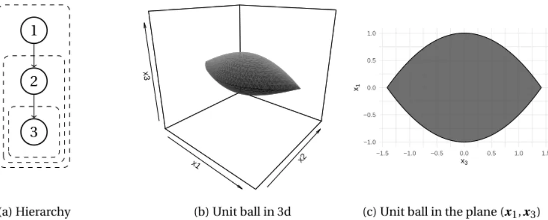
The elastic-net penalty was introduced by ?:

λ¡αkβk2

2+ (1 − α) kβk1¢ (1.19)

whereα ∈ [0,1] is an hyper-parameter to be fixed. The elastic-net penalty defines a norm that is a compromise between the L1 and the L2 norm: asα varies, the elastic-net estimate varies

continu-ously between the lasso and the ridge estimates. Forα = 0 it becomes the lasso penalty and for α = 1 it becomes the ridge penalty.

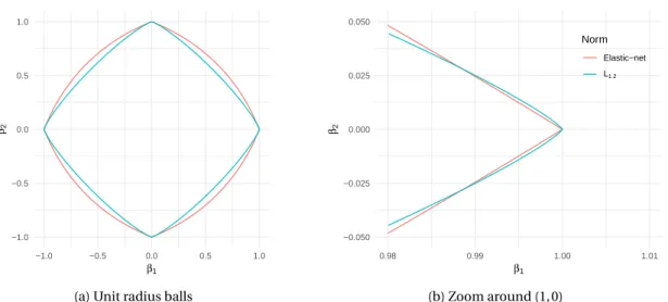
Contrarily to the Lq norm (1 ≤ q ≤ 2), the elastic-net penalty is non-differentiable, as illustrated

in Figure 1.4. Consequently, the elastic-net always performs selection (forα 6= 1) like the lasso and shrinkage like the ridge (which reduces the MSE). Comparatively, the Lq norm (1 < q < 2) does not

perform model selection and is of little interest. We emphasize that it is thanks to its singularity at zero that the elastic-net performs variable selection. In fact, this property is central to all sparsity-inducing penalties, as will be discussed in more details in Section 1.1.7. As discussed hereafter, the elastic-net enjoys the desirable properties from both estimates.

The thresholding function of the elastic-net under orthogonal design is

ˆ βen i = (| ˆβols_i | − λ1/2)+ 1 + λ2 sgn{ ˆβols_i }. (1.20)

This thresholding function has the same behavior as the soft thresholding for small values of ˆβols_i and the same behavior as the ridge thresholding for large values of ˆβols_i . An illustration is given in Figure 1.7 withλ1= 2 and λ2= 1.

The elastic net is also more stable in selection than the lasso. More precisely, if several covariates are very correlated, the lasso will arbitrarily select one covariate and discard the others. This is proven (?) not to be the case for the elastic-net: the difference¯¯β_i− β_j

¯

¯is bounded by 1 − corr{x_i, x_j}, so that highly correlated covariate effects have close to equal estimates. This property is known as the

grouping effect: the elastic net selects important covariates in group.

Moreover, in the p À n scenario, lasso does not perform well in selection because it cannot select more than n covariates. The elastic-net overcomes this obstacles and, even with smallα, can select any number of covariates.

Finally, the elastic-net estimate writes also as the minimizer of

βTµXTX + λ2I 1 + λ2 ¶ β − 2XT y + λ1 ° °β°°₁, (1.21)

hence it is computed as a lasso estimate with a modified design matrix.

The LARS algorithm can be adapted to estimate the elastic-net. Recall that LARS computes the whole regularization path. Thus the LARS algorithm is called on a grid of values ofλ2and the selected

value is the one which minimizes the (ten-fold) cross-validation error. The computational cost of this procedure is K times more than that of a lasso fit, where K is the length of the grid ofλ2.

1.1.4 Bridge regression

Bridge regression is based on the Lqpenalty:

ˆ

βbridge,arg min

β `¡β¢ + λ p X j =1 ¯ ¯β_j ¯ ¯γ (1.22)

whereγ > 0 is a parameter to be fixed. Bridge regression was first introduced by Frank and Friedman (1993) as a generalization of the ridge (γ = 2) and the lasso (γ = 1) and was later studied by Fu (1998), who compared it with the lasso. For 0 < q ≤ 1 the Lq penalty is singular around zero and the bridge

(30)

−1.0 −0.5 0.0 0.5 1.0 −1.0 −0.5 0.0 0.5 1.0 β1 β2

(a) Unit radius balls

−0.050 −0.025 0.000 0.025 0.050 0.98 0.99 1.00 1.01 β1 β2 Norm Elastic−net L1.2 (b) Zoom around (1, 0)

Figure 1.4: Illustration of why the elastic net induces sparsity and not the Lq norm (1 < q < 2). Unit

radius balls of the elastic-net norm (α = 0.2) and the L1.2norm.

regression performs variable selection. This property is illustrated in Figure 1.2 which represents unit balls of Lqnorms for different values of q.

Asymptotic properties of the bridge regression has been studied by Knight and Fu (2000) in both casesγ ≤ 1 and γ > 1.

Fu (1998) proposed an algorithm based on the Newton-Raphson procedure to compute the bridge estimate whenγ > 1. However, when 0 < γ < 1, the penalty is not convex and its minimization is com-putationally challenging.

The bridge penalty is part of a general family of sparsity inducing penalties called non-concave penalties These are defined in the next section. The oracle properties of the bridge estimate and the algorithms available to compute it are given in this section.

1.1.5 Berhu

The Berhu penalty was introduced by Owen (2006):

p_λ(|θ|) = ( |θ| |θ| ≤ λ θ2_+λ2 2λ |θ| > λ (1.23)

It is equal to the absolute value around zero and is quadratic away from zero. Consequently it is sometimes referred to as inverse Huber function (Huber et al., 1964).

The presence of the singularity of the penalty at zero makes it a variable selection method. The Berhu penalty replaces the absolute value penalty by a quadratic penalty for large values in order to benefit from the properties of the ridge regression: the grouping effect, and an increased accuracy in estimation. The Berhu penalty can be seen as mixing the L1and L2penalties; in this regards it is very

similar to the elastic-net.

1.1.6 Penalized likelihood methods as a Bayesian prior

Let the variableM denote the model. Recall that in the Bayesian framework, the data are generated from a model which is also assumed to be random. The distribution of the model is an a priori information that we must provide. The goal of Bayesian inference is to infer the posterior likelihood P(M |data). From the Bayes formula:

P(M |data) =P(data|M )π(M )

(31)

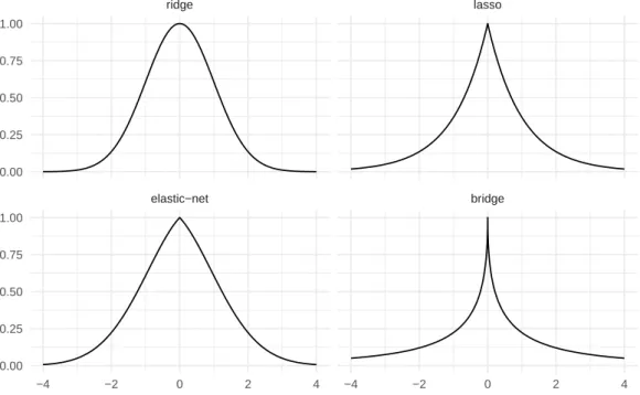
elastic−net bridge ridge lasso −4 −2 0 2 4 −4 −2 0 2 4 0.00 0.25 0.50 0.75 1.00 0.00 0.25 0.50 0.75 1.00

Figure 1.5: Bayesian priors on the parameter with the Ridge, Lasso, Elastic-net (α = 0.5), and Bridge (q = 0.5) penalties.

whereπ(M ) is the prior distribution of the model, which includes a priori information about the model distribution.

Here, the symbol for probability must be understood in the sense of density. The prior on the data does not intervene in the minimization of the integrated negative log-likelihood. The first prob-ability in the right-hand side of (1.24) is the likelihood (of the data). In this case, the modelM is the parameterβ from which the data is generated. Then, Bayesian inference is made by minimizing:

−2 log P¡β|data¢ = 2`¡β¢ − 2logπ(β), (1.25) where we recall that`(β) is the negative log-likelihood (of the data conditionally on the model). Equation 1.25 is very similar to penalized maximum likelihood estimation. Notice that Equations (1.25) and (1.5) are the same on the condition that

−2 log π¡

β¢ = λkβk2_.

Consequently, the ridge penalty can be seen as a Bayesian inference with a normal prior distribution on the parameter: β ∼ N ¡0,λ2¢. The hyper-parameterλ is the standard deviation of the centered

normal prior on the parameter. More generally, the Lqnorm penalty corresponds to the prior

π(β) = exp Ã −λkβk q q 2 ! .

The lasso regression corresponds to a prior on the parameter with a Laplace distribution. These priors are represented in Figure 1.5 in the univariate case. Likewise, the elastic-net corresponds to the prior π¡β¢ ∝ exp Ã −λαkβk 2 2+ (1 − α)kβ1k 2 ! ,

(32)

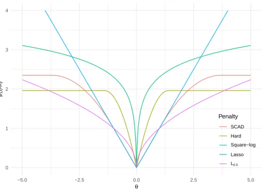
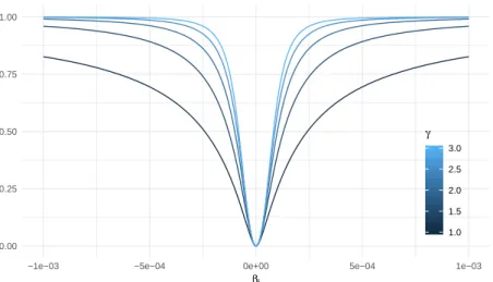
0 1 2 3 4 −5.0 −2.5 0.0 2.5 5.0 θ pλ (l θ l) Penalty SCAD Hard Square−log Lasso L0.5

Figure 1.6: Several non-concave penalties with different values ofλ. 1.1.7 Non-concave penalties

Forword. In this section, we will define a family of penalties that enforce variable selection. As is

explained hereafter, these penalties have the minimal set of properties to enforce variable selection. They include many of the previously mentioned variable selection penalties: the lasso, the bridge, and the Berhu (other non-concave penalties are also introduced in this section). As such, the tools used to compare non-concave penalties are of importance when comparing variable selection meth-ods. Non-concave penalized estimates are defined as the minimizers of

`¡β¢ + p X j =1 p_λ¡¯ ¯β_j ¯ ¯ ¢ (1.26)

where p is a non-concave function, or non-concave penalty, in the following sense.

Definition 3 (Non-concave function). A real-valued function p_λ(|θ|) defined on R is said to be

non-concave if it is (i) even onR with p_λ(0) = 0 (ii) non-decreasing and concave on (0,∞) (iii) differentiable

overR∗.

The differentiability condition can be relaxed to piecewise differentiability without without loss of generality. Since it is not a restrictive assumption in practice, we will assume differentiability for the sake of the presentation. We emphasize the fact that in this work, the term “non-concave” is not used to say that a function is not concave.

In the cases where p_λ(|βj|) is proportional to λ, we will denote pλ(|.|) byλp(|.|) and drop the

indexλ. One may also want to penalize some variables more than others, because of some a priori knowledge about their importance. This is done by setting a different penalty for each coefficient. For the sake of the presentation, we will assume that all the components ofβ are penalized the same. The estimates defined by (1.26), where p_λis a non-concave penalty, will be called non-concave estimates. Many important sparse estimates write as non-concave estimates, which makes (1.26) a good framework to analyze and compare sparsity-inducing penalized likelihood methods. Using the definition of non-concave penalty, we can (i) give conditions on the penalty for the corresponding

(33)

SCAD Ridge Elastic−net

Hard Soft Adaptive ridge

−4 −2 0 2 4 −4 −2 0 2 4 −4 −2 0 2 4 −4 −2 0 2 4 −4 −2 0 2 4

(34)

estimate to be sparse, (ii) give theoretical results shared by non-concave sparse estimates, (iii) com-pare the behavior and performance of sparsity-inducing estimates by comparing their corresponding penalty functions.

The lasso and the bridge (0 < q < 1) are both non-concave estimates ; this follows directly from (1.12) and (1.22) respectively. In the following sections we define two important non-concave penal-ties: the hard-thresholding and the smoothly clipped absolute deviation (SCAD). Figure 1.6 rep-resents several non-concave penalties. Since non-concave penalties are concave and decreasing on (0, ∞), they verify p0(0+) > 0. Since they are even functions, we also have p0(0−) < 0. Thus by definition, they are not differentiable at 0. This property is proven (?) to be a sufficient condition for a penalty to perform variable selection. Thus all non-concave penalties such that p0_λ(0+) > 0 perform variable selection.

Figure 1.6 illustrates the shapes of several non-concave penalties. The sharper the penalty, the better it approximates the L0norm, which is the desired penalty. However, sharp penalties are harder

to minimize, which makes the estimation procedure more computationally intensive. First, penalties like the SCAD and hard-thresholding, which are constant away from zero, are hard to minimize. The lasso is an outstanding non-concave penalty: it is minimally non-concave, since it is linear on (0, ∞), which is the least concave function. Moreover, the derivative of the L1penalty is constant on (−∞,0)

and (0, ∞) and thus its minimization cannot be performed using classic optimization methods. Fi-nally, note that empirically, the sharper the spike around zero, the “stronger” the estimates will be enforced to be sparse.

Figure 1.7 represents the thresholding functions of some non-concave penalties under the case of orthogonal design: ˆβj= f ( ˆβols_j ) = f (XTy). Asymptotically the variables with a non-zero effect on

y will have an OLS estimate far away from zero and the variables with no effect on y will be around

zero. Consequently, the penalty

(i) Performs variable selection only if the thresholding function is identically equal to zero around a neighborhood of zero;

(ii) Estimates the non-zero effect without bias only if the thresholding function is close to the iden-tity function (dotted lines on the figure) for large values of the data.

(iii) Is stable in selection if the thresholding function is continuous. (By stable we mean that the selected model is not highly sensitive to small variations in the data.)

The convergence properties of the non-concave penalties was studied by ?. Under mild regularity conditions onλn and pλthe non-concave penalties have the oracle properties. The only restrictive

condition is that

lim sup

n→∞ lim supθ→0 p

0

λn(θ)/λn> 0. (1.27)

The minimization of non-concave functions is a computationally difficult task. Derivative-based optimization methods are not efficient in this context, because (i) the derivative of the penalty is not always continuous and (ii) the second order derivative p_λ00(|θ|) takes infinitely small values. Specific optimization methods have to be used to derive numerical estimation procedures that are stable and fast to compute. These methods are introduce in the framework of MM optimization, in Section 1.3.1.

1.1.7.1 Hard-thresholding

Consider the L0penalty

p_λ(|θ|) = λ21θ6=0, (1.28)

also called the entropy penalty.

Note that in orthogonal design, the penalized least squares is¡ yi− βi¢2+ λ21βi6=0, and since kxk0

(35)

is taken at 0 whenλ2< y_i2. Thus, the thresholding function of the L0penalty is the so-called hard

thresholding rule (Figure 1.7):

ˆ

βhard

= β1|β|<λ. (1.29)

This thresholding only clips the values below the thresholdλ to zero, and leaves the other values unmodified. As discussed, this penalty makes the computation of the estimation NP-hard.

Let us now consider the penalty function

p_λ(|θ|) = λ2− (|θ| − λ)21|θ|<λ. (1.30)

Surprisingly, under orthogonal design, this penalty also gives the hard thresholding rule (see An-toniadis, 1997; Fan, 1997). Since it is a much simpler quantity to minimize, this penalty is used when we want to have an unbiased variable selection method. This penalty is also referred to as hard thresholding penalty; it is represented in Figure 1.6.

The discontinuity in the hard thresholding makes the model selection unstable. The next penalty offers to remedy this problem, while still having an unbiased estimate of the parameters.

1.1.7.2 SCAD

The smoothly clipped absolute deviation (SCAD) penalty was introduced by Fan (1997) and analyzed by ?. It is defined by p0_λ(¯¯β¯¯_j) = λI ¡ βj≤ λ¢ + λ ¡aλ − βj¢₊ (a − 1)λ I ¡ βj> λ¢ , (1.31)

for some a > 2 and for βj > 0. This penalty is linear over [0, λ], parabolic over [λ, aλ], and

con-stant over [aλ,∞). Therefore it behaves like the lasso for small values of the data and like the hard-thresholding penalty for large values of the data. Under orthogonal design, the SCAD has the follow-ing thresholdfollow-ing function (see Figure 1.7):

ˆ βj=        sgn¡ βj¢ ³_¯ ¯β¯¯_j− λ ´ + when ¯ ¯β_j ¯ ¯< 2λ ©(a − 1)βj− sgn¡βj¢ aλª/(a − 2) when 2λ < ¯¯βj

¯ ¯≤ aλ βj when ¯ ¯β_j ¯ ¯> aλ (1.32)

This thresholding rule equals that of the lasso for¯¯β_j ¯

¯< λ and equals the hard thresholding for ¯ ¯β_j

¯ ¯>

aλ.

In addition toλ, the parameter a also needs to be determined. We can use cross-validation over a two-dimensional grid, but the computational cost can be deterrent. ? performed simulations under orthonormal design with a prior distributionβj∼iidN (0,aλ) and estimated the L2riskE[k ˆβ−β∗k2].

They proposed to take the value a = 3.7 and noted that the risk does not vary a lot for different values of a.

Note that the SCAD is the only non-concave penalty which is not proportional toλ. This has no influence on the minimization of (1.26) for a fixed value ofλ. However, this can make it more complicated to minimize (1.26) for a sequence of values ofλ. This difference can make the added computational cost of the SCAD deterrent. We refer to Zou and Li (2008) for more details.

1.1.7.3 Logarithmic penalty

In order to recover highly sparse estimates, non-concave penalties are required to have a “sharp” spike at zero, or in other words, to have a derivative that vanishes away from zero. We have discussed that penalties which are constant away from zero are harder to minimize. An obvious and simple choice is then to use the logarithmic function as a penalty:θ 7→ log(|θ|). Since the logarithm equals −∞ at zero, this function does not comply as a penalty function. To remedy this issue, we cap the log function away from −∞ in the following manner: define the “log penalty”