HAL Id: tel-01676953
https://hal.archives-ouvertes.fr/tel-01676953v2
Submitted on 6 Feb 2019
HAL is a multi-disciplinary open access
archive for the deposit and dissemination of sci-entific research documents, whether they are pub-lished or not. The documents may come from teaching and research institutions in France or abroad, or from public or private research centers.
L’archive ouverte pluridisciplinaire HAL, est destinée au dépôt et à la diffusion de documents scientifiques de niveau recherche, publiés ou non, émanant des établissements d’enseignement et de recherche français ou étrangers, des laboratoires publics ou privés.
To cite this version:
Amina Doumane. On the infinitary proof theory of logics with fixed points. Logic in Computer Science [cs.LO]. Université Sorbonne Paris Cité, 2017. English. �NNT : 2017USPCC123�. �tel-01676953v2�
Ecole Doctorale 386 — Sciences Mathématiques de Paris
Centre
Laboratoire IRIF, Equipe PPS
On the infinitary proof theory of
logics with fixed points
par
Amina Doumane
Thèse de doctorat en informatique fondamentale
Dirigée par Pierre-Louis Curien, David Baelde et Alexis Saurin
Présentée et soutenue publiquement à Paris Diderot le 27 Juin 2017
David Baelde
Co-directeur de thèse
Arnaud Carayol
Examinateur
Pierre-Louis Curien
Directeur de thèse
Martin Hofmann
Rapporteur
Delia Kesner
Examinateur
Luke Ong
Rapporteur
Alexis Saurin
Co-directeur de thèse
Igor Walukiewicz
Président du jury
Logique et informatique La logique, et plus spécifiquement la théorie de la démonstra-tion, a été particulièrement utile en informatique, en particulier en langages de programma-tion et en vérificaprogramma-tion formelle.
D’une part, la théorie de la démonstration a profondément révolutionné le domaine des langages de programmation via les deux paradigmes de calcul suivants: la programmation fonctionnelle et la programmation logique. En programmation fonctionnelle, pour garan-tir que les programmes terminent, il est usuel de considérer des langages typés. Dans ces langages, les programmes correspondent aux preuves, les types aux formules logiques et l’exécution à l’élimination des coupures. Cette dernière propriété est au cœur de cette cor-respondance, appelée l’isomorphisme de Curry-Howard. En programmation logique, un pro-gramme est un ensemble de formules logiques et un calcul consiste à décider si une formule, appelée requête, est une conséquence logique du programme. Le paradigme de calcul est donc la recherche de preuve. Pour que celle-ci soit efficace, le système de preuve sous-jacent doit vérifier les deux propriétés fondamentales que sont l’admissibilité de la coupure et la focalisation. Les deux propriété logiques fondamentales qui assurent le lien entre logique et langages de programmation sont donc l’élimination des coupures et la focalisation. D’autre part, en vérification formelle, la logique est utilisé comme un outil pour décrire les système et leurs propriétés. Même si le model-checking est le paradigme dominant en vérification, une approche, dite preuve-théorique, commence a regagner de l’intérêt. Elle consiste à décrire à la fois le système et la propriété à vérifier par des formules S et P , puis vérifier que le système satisfait la propriété consiste à vérifier si la formule S → F est prouvable. L’intérêt de cette approche est que la preuve résultante de S → F peut être utilisée comme un certificat, qui peut être indépendamment communiqué et vérifié.
Logiques à points fixes L’extension des logiques avec des points fixes est particulière-ment intéressante en informatique. En programmation, les points fixes permettent un traite-ment direct, générique et intuitif des types de données (co-)inductifs comme les entiers na-turels, listes, stream, etc. En vérification, une des logiques les plus utilisée est le mu-calcul, qui est une logique modale avec points fixes. Il est donc naturel de s’intéresser à la théorie de la démonstration des logiques à points fixes. Systèmes de preuves pour les logiques à points fixes Il existe deux grandes familles de systèmes de preuves pour les logiques à points fixes: les systèmes de preuves finitaires et les systèmes de preuves infinitaires.
• Dans les Systèmes de preuve finitaires, les règles pour les points fixes reflètent les principe de (co-)induction. Ces systèmes de preuve, quoique très largement utilisés, représentent plusieurs inconvénients. Le premier est que la règle de coupure est in-évitable, par conséquent ces systèmes ne sont pas adaptés à la recherche de preuve.
Un autre inconvénient est que leur contenu calculatoire n’est souvent pas explicite et il est en général difficile de deviner ce qu’une preuve calcule, de savoir si deux preuves calculent la même fonction, etc.
• Dans les systèmes de preuves infinitaires, les règles pour les points fixes sont de simples règles de “déroulages”, mais les preuves peuvent avoir une profondeur infinie. Ils sont plus adaptés à la recherche de preuve, et les règles de déroulage ayant un comportement calculatoire facile à analyser, le contenu calculatoire des preuves infinitaires est souvent explicite.
Même si les systèmes infinitaires existent depuis longtemps, ils ont été utilisés principalement comme des outils techniques et n’ont pas été considérés comme de vrai systèmes de preuves. Ceci est dû à un manque de résultats fondamentaux (élimination des coupures, focalisation) qui nous empêche de les voir comme tel. L’objectif de cette thèse est de pallier à cette lacune dans l’état de l’art, en développant la théorie de la démonstration infinitaire pour les logiques a points fixes, avec deux domaines d’application en vue: les langages de programmation avec types de données (co-)inductifs et la vérification des systèmes réactifs.
Contributions de la thèse Cette thèse peut être résumée comme suit: Les logiques à points fixes peuvent être équipées de systèmes preuve infinitaires qui ont un réel statut preuve-théorique et peuvent être appliquées à d’autres domaines comme la vérification formelle.
Naturellement, cette thèse est divisée en deux parties. Dans la première, on argumente le fait que les preuves infinitaires ont effectivement un réel statut preuve-théorique, en montrant qu’ils admettent les propriétés d’élimination des coupures et de focalisation. Dans la deuxième partie, on utilise nos développements sur les preuves infinitaires pour monter de manière constructive la complétude du mu-calcul linéaire relativement à l’axiomatisation de Kozen. Ces deux parties sont précédées par une partie introductive qui expose 1) nos choix de design, 2) un peu de background sur les systèmes de preuves pour les points fixes et 3) un outil technique qui sera très utile tout au long de la thèse: un résultat de traduction entre les systèmes finitaires et infinitaires.
Partie I: Étude preuve-théorique des logiques à points fixes Comme d’habitude, étudier les propriétés preuves théoriques dans un cadre linéaire permet de s’abstraire de beaucoup de bruit et de se focaliser sur les vrai difficultés. Aussi nous avons décidé d’établir les propriétés d’élimination des coupures et de focalisation dans le cadre de la logique linéaire additive multiplicative. Dans le Chapitre 3, nous utilisons une nouvelle technique de preuve pour établir élimination des coupures pour notre système infinitaire. A la fin du Chapitre 3, on indique comment étendre ce résultat pour la logique linéaire classique et la logique classique. Dans le Chapitre 4, nous établissons la propriété de focalisation en analysant les phénomènes qui apparaissent dans le cadre infinitaires comparé au cadre finitaire. Le Chapitre 5 est dédié à un autre problème: élucider le contenu calculatoire des preuves fini-taires. Pour ce faire, on muni la logique linéaire multiplicative additive avec une sémantique dénotationnelle, pour laquelle on montre un résultat de complétude partiel. Chemin faisant, on montre la décidabilité et la complétude de l’inclusion sémantique.
Partie II: Complétude constructive pour le mu-calcul linéaire Dans son papier fondateur, Kozen en a proposé une axiomatisation pour le mu-calcul, dont la complétude a été montré 13 ans plus tard par Kaivola dans le cas linéaire et par Walukiewicz dans le cas branchant. Ces preuves de complétude sont basées sur des arguments complexes et non constructifs, qui ne donnent aucun moyen de construire une preuve pour une formule valide. La problématique de constructivité devient centrale lorsqu’on considère les preuves comme des certificats pour les outils de vérification formelle. Nous proposons une nou-velle preuve de complétude pour le mu-calcul linéaire qui est constructive, càd qui construit une preuve pour toute formule valide. Pour ce faire, nous décomposons ce problème dif-ficile en plusieurs sous-problèmes en utilisant la correspondance entre le mu-calcul et les automates. Plus précisément, on relève les transformations d’automates comme la déter-minisation et l’élimination de l’alternance au niveau de la logique. Pour résoudre chacun des sous-problèmes, on fait une recherche de preuve dans un système infinitaire, puis on transforme chaque preuve infinitaire obtenue en une preuve dans l’axiomatisation de Kozen en utilisant notre résultat de transformation de la partie introductive.
The subject of this thesis is the proof theory of logics with fixed points, such as the µ-calculus, linear-logic with fixed points, etc. These logics are usually equipped with finitary deductive systems that rely on Park’s rules for induction. other proof systems for these logics exist, which rely on infinitary proofs, but they are much less developped. This thesis contributes to reduce this deficiency by developing the infinitary proof-theory of logics with fixed points, with two domains of application in mind: programming languages with (co)inductive data types and verification of reactive systems.
This thesis contains three parts. In the first part, we recall the two main approaches to the proof theory for logics with fixed points: the finitary and the infinitary one, then we show their relationships. In the second part, we argue that infinitary proofs have a true proof-theoretical status by showing that the multiplicative additive linear-logic with fixed points admits focalization and cut-elimination. In the third part, we apply our proof-theoretical investigations to obtain a constructive proof of completeness for the linear-time µ-calculus w.r.t. Kozen’s axiomatization.
Contents 7
Introduction 11
1 Background on proof theory 25
1.1 Syntax, semantics and proof systems . . . 25
1.2 Propositional classical logic . . . 26
1.2.1 LKformulas . . . 26
1.2.2 Semantics of LK formulas . . . 26
1.2.3 The proof systems LK, LKrev and LKos . . . 27
1.3 Linear Logic . . . 31
1.3.1 MALLformulas . . . 32
1.3.2 The proof system MALL . . . 33
1.3.3 LL formulas . . . 33
1.3.4 The proof system LL . . . 34
1.3.5 Semantics of MALL and LL formulas . . . 34
1.4 Linear temporal logic . . . 35
1.4.1 LTL formulas . . . 36
1.4.2 Semantics of LTL formulas . . . 36
1.4.3 Proof systems for LTL . . . 37
1.5 On the shape of sequents . . . 37
1.5.1 Review on the shape of sequents . . . 37
1.5.2 Sequents as sets of formula occurrences . . . 39
2 Fixed-points in proof theory 43 2.1 Fixed points theorems . . . 43
2.2 Formulas with fixed points . . . 46
2.3 On the notion of subformula . . . 47
2.3.1 The usual notion of subformula . . . 47
2.3.2 Fischer-Ladner subformulas . . . 49
2.3.3 Comparing FL-subformulas . . . 51
2.4 Proof systems for logics with fixed points . . . 55
2.4.1 Finitary proof system . . . 56
2.4.2 Infinitary proof system . . . 60
2.4.3 Circular proof system . . . 63
2.4.4 From finitary to circular proofs . . . 70
2.4.5 From circular to finitary proofs . . . 73
I Linear logic with least and greatest fixed points
85
3 Cut-elimination for µMALL∞ 87 3.1 Reduction rules . . . 883.1.1 The multicut rule . . . 89
3.1.2 Reduction rules . . . 90
3.1.3 Reduction sequences . . . 92
3.1.4 Statement of the cut-elimination theorem and proof sketch . . . 94
3.2 Extracting proofs from reduction paths . . . 94
3.3 Truncated truth semantics . . . 98
3.3.1 Truncated semantics . . . 98
3.3.2 Soundness w.r.t. truncated semantics . . . 99
3.4 Productivity of the cut-elimination process . . . 103
3.5 Preservation of validity by cut-elimination . . . 103
3.6 Examples . . . 105
3.7 Extensions of the cut-elimination result . . . 107
3.7.1 Treatment of atoms . . . 107
3.7.2 Extension to µLLω, µLKω and µLK⊙ω . . . 107
4 Focalization of µMALL∞ proofs 109 4.1 Polarity of connectives . . . 111
4.2 Reversibility of negative inferences . . . 112
4.3 Focalization of positives . . . 114
4.4 Productivity and validity of the focalization process . . . 118
4.5 Example . . . 119
5 Ludics for linear logic with fixed points 121 5.1 Polarized linear logic with fixed points . . . 122
5.1.1 Formulas . . . 122
5.1.2 The proof system µMALLP . . . 122
5.2 Computational ludics . . . 126
5.2.1 Designs . . . 126
5.2.2 Cut-elimination and Orthogonality . . . 128
5.2.3 Behaviours, Sets of Designs . . . 129
5.2.4 Designs as Strategies . . . 130
5.3 Interpretation of µMALLP in Ludics . . . 130
5.3.1 Interpretation of Formulas . . . 130
5.3.2 Interpretation of µMALLP Proofs . . . 132
5.3.3 Soundness and Invariance by Cut Elimination . . . 134
5.4 On Completeness . . . 137
5.4.1 Essentially finite designs . . . 137
II Constructive completeness for the linear-time
µ-calculus
145
6 The completeness problem for the linear-time µ-calculus 147
7 The linear-time µ-calculus 153
7.1 Syntax and semantics . . . 154
7.2 Proof systems for the linear-time µ-calculus . . . 155
8 Automata over infinite words 159 8.1 Alternating and (non-)deterministic automata . . . 159
8.1.1 Alternating automata . . . 160
8.1.2 Non-deterministic automata . . . 163
8.1.3 Deterministic automata . . . 164
8.2 Comparing ω-automata . . . 165
9 Alternating parity automata and the µ-calculus 169 9.1 Operational semantics . . . 169
9.2 From APW automata to formulas . . . 171
9.2.1 The encoding . . . 172
9.2.2 Fischer-Ladner subformulas of the encoding . . . 176
9.3 From formulas to APW automata . . . 178
9.4 A formula and the encoding of its automaton are equivalent in µLK⊙ . . . . 181
10 Alternation elimination and parity simplification 185 10.1 From APW to NPW . . . 185
10.1.1 Non-determinization . . . 185
10.1.2 Non-determinization in the logic . . . 187
10.2 From NPW to NBW . . . 189
10.2.1 Parity simplification . . . 189
10.2.2 Parity simplification in the logic . . . 189
11 Büchi inclusions in µLK⊙ 193 11.1 Power-set construction in the logic . . . 194
11.2 Parity automata inclusions in µLK⊙ω . . . 196
11.3 Büchi automata inclusions in µLK⊙ . . . 204
11.3.1 Weakly deterministic formulas . . . 205
11.3.2 Büchi inclusions . . . 207
12 Constructive completeness 211 12.1 Picking up all the pieces . . . 211
12.2 Discussion . . . 213
Conclusion 217
“On the unusual effectiveness of logic in computer
science”
Even if logic has its roots in Ancient Greece with Aristotle’s work, formal logic, as we know it, was born in the early 20th century to confront the crisis in the foundations of mathematics, brought about by the paradoxes of set theory. In his famous program, Hilbert was intending to show that mathematics are consistent and decidable by formalizing them. The works on logic of the time [Gö31, Tar35, Chu36, Tur36] showed that most of Hilbert’s goals were impossible to achieve. Since then, mathematics and logic have followed their own paths. Nowadays, logic is considered as a mature and independent research area, with many fields of application. The most striking example of such an application is certainly computer science, which was heavily influenced by logic’s development. We discuss in the following two areas of computer science where logic is particularly successful: programing languages which were influenced by the proof theoretical side of logic and formal verification which benefited most from its model theoretical one.
Logic and programming languages. Proof theory impacted strongly the domain of programming languages through the two following paradigms of computation: functional programming and logic programming.
• Functional programming and the Curry-Howard approach. The prototype of a functional programming language is λ-calculus introduced by Church [Chu32,Bar84]. A well-designed functional programming language is a language where programs should be safe by construction. Safe means that the program does not raise an error during its execution, due for instance to a function called with too few arguments or with arguments with the wrong types. A way to ensure this safety property is to consider type-based programming languages, in which well-typed programs “cannot go wrong” as summarized by Milner’s slogan. Type systems have an intriguing similarity with proof systems. Much more than a mere coincidence, this similarity is a general fact known as the Curry-Howard correspondence. This correspondence exhibits an isomorphism between a number of programming languages and various proof systems. Let us briefly review the three main styles in which proof systems come:
– Hilbert-style systems are given by a set of axioms reflecting the properties of the logical connectives. One can derive from these axioms new theorems using the
modus ponens rule:
A ⇒ B A
(modus ponens)
B
– Natural deduction was introduced by Gentzen in 1935, and it is the formalism that reproduces most faithfully the mathematical reasoning (hence the attribute “Natural”). It is not axiomatic in the sense that the properties of the connectives are not reflected by axioms, but instead by means of inferences rules. Inference rules for connectives can either introduce a connective or eliminate it. A proof is a tree of formulas, where each node is justified by an introduction or elimination rule and each leaf is called a “hypothesis”. Some leaves of the tree are discharged, meaning that they are not to be considered as hypothesis. If all leaves are dis-charged, then the conclusion holds without hypothesis. We call cut a pattern formed by an introduction rule for a connective followed immediately by an elim-ination rule for this connective. Cuts are somehow detours in the proof. To show that cuts can be eliminated from natural deduction proofs, Gentzen introduced another formalism of proofs: sequent calculus.
– Sequent calculus is based on the notion of sequent which generalizes that of formula: a sequent has the form Γ ⊢ ∆ where Γ and ∆ are two lists of formulas, and it can be understood as “the conjunction of the elements of Γ implies the disjunction of the elements of ∆” (the symbol ⊢ can be thought of as an impli-cation). The inference rules for connectives can either introduce a connective on the right or on the left of the sequent; and a proof is a tree of sequents built using inference rules. In sequent calculus, the cut is not a pattern of rules, as in natural deduction, but it is a proper rule of the system:
∆1 ⊢ Γ1, A A, ∆2 ⊢ Γ2
(Cut)
∆1, ∆2 ⊢ Γ1, Γ2
Gentzen showed that cuts can be eliminated from sequent calculus proofs using an effective procedure. Prawitz showed the same result for natural deduction proofs.
These results are the heart of the Curry-Howard correspondence, the latter being not simply a mapping between proofs and programs, and between formulas and types, but also, and more importantly, an isomorphism between the cut-elimination procedure (or any other form of proof normalization) and the execution of programs.
The first instance of this correspondence was discovered by Curry, who established in 1958 an isomorphism between Hilbert style proof systems and combinatorial logic, here the use of modus ponens corresponds to the application of combinators. Later, in 1969, Howard pointed out the correspondence between minimal logic in natural deduction and simply-typed lambda calculus [How80]. Since then, the Curry-Howard correspondence has been extended to other frameworks, either by enriching the logic (for instance, Girard and Reynolds [Gir72,Rey74] discovered a correspondence between second-order logic and polymorpism, and Griffin [Gri90] discovered that Felleisen’s control operator C [FFKD87] can be typed with ¬¬A ⇒ A, which was a stepping stone for the Curry-Howard extension to classical logic); or by exploring other formalisms
of proofs (for instance by considering a Curry-Howard correspondence for sequent calculus [CH00]).
Over time, the meaning of the Curry-Howard correspondence has evolved from the simple observation of an isomorphism between an existing proof system and an existing programming language, to something more “productive”. Indeed, one can either start from a typed programming language and extract its isomorphic proof system which may have an interesting logical meaning. Conversely, one could start from a known proof system and try to understand its computational content in order to design its corresponding programming language, this is for instance how a number of calculi were born [Par92, CH00, MM09].
Curry-Howard was also productive in renewing questions related to the semantics of logic, putting an emphasis on the semantics of proofs, in contrast to tranditional thruth or provability semantics. In this sense, linear logic [Gir87] arose from Girard’s study of the denotational semantics of system F.
• Logic programming. This paradigm of computation orginated directly from logical considerations. Here, a program is a set of logical formulas, and a computation is performed by deciding whether a formula, called a query, is a logical consequence of the program or not.
The most popular example of a logic programming language is Prolog [SS86]. Its formulas are described using first-order Horn clauses, and its execution proceeds as follows: to decide whether a query is a consequence of the program, it adds its nega-tion the program, and searches for a proof of false. This proof-search uses the SLD resolution technique [VEK76], which amounts to search for a clause that allows to con-clude immediately the goal (initially this goal is false), in which case the proof-search continues with the hypothesis of this clause as goals, etc.
In [MNPS91], Miller et al. characterize, in a generic way, what a Logic Programming language is. This is done through the notion of uniform proofs. A uniform proof is one that can be found by a goal-directed search. This generic vision of a logic program-ming language allowed to reformulate existing languages (such as Prolog) in proof-theoretical terms. It allowed also to design new languages such as λ-Prolog [MN12], by going from first-order Horn clauses to higher-order hereditary Harrop formulas. This idea of uniform proofs had another fundamental consequence: when trying to extend it to linear logic, Andreoli came across focalization [And92]. While reversible connectives (that is, the connectives that can be applied without risking the loss of provability) are known to behave well in proof-search, the focalization result shows that non-reversible connectives have also good properties. This result has had sev-eral applications in both logic (it is at the heart of polarized linear logic [Lau02], and ludics [Gir01, Ter11]) and programming languages much beyond logic program-ming (it gave new insights on our understanding of evaluation order of programprogram-ming languages [DJS97], CPS translations, and pattern matching [CM10, Zei09]).
Formal verification. In programming languages, logic is a tool internal to the computa-tion paradigm: typing rules are the building blocks to construct (safe) funccomputa-tional programs and formulas are the building blocks of logic programs. In formal verification, logic is used as
an external tool to describe existing computer systems, and make formal statements about them.
One of the most successful approaches to verification is model checking [CE81]. In this approach, the system is described by a mathematical structure M and the property to check about it is represented by a formula ϕ in a certain logic. Then checking whether the system satisfies the property amounts to check whether M is a model of ϕ, that is M |= ϕ. In this approach, the choice of the logical language is very crucial. On the one hand, it should be expressive enough to describe complex behaviours of the system. On the other hand, the problem of deciding whether a model satisfies a formula should be decidable, and preferably with a reasonable complexity. Temporal logics [Pnu77] are one of the more widely used specification languages in this sense, and Linear Temporal logic (LTL) and Computation tree logic (CTL*) are cases in point.
The temporal modalities of LTL are ⊙ (in the next moment of time) G (always) and F (eventually); formulas are built using these temporal modalities combined with proposi-tional connectives and atomic propositions. For instance, the LTL formula FGϕ means that “eventually, ϕ will always holds”. The models of LTL formulas are linear structures. We can extend this interpretation to branching structures, by setting M |= ϕ if for every path p of M, we have that p |= ϕ. Thus, there is an implicit universal quantification on paths in LTL formulas. The logic CTL* allows both universal and existential quantification, through the path quantifier ∀ (in all paths) and ∃ (for some path); CTL* formulas are build using these path quantifiers combined with LTL connectives. For instance, the CTL* formula ∃Gϕ means that “There is a branch of the model where ϕ always holds”. The use of CTL* and LTL goes beyond the academic frame, and finds a considerable industrial success throught tools such as SMV and VIS, FormalCheck, etc, with many applications in major software companies (IBM, Intel, Microsoft, etc).
There is another approach to verification that lives in the shadow of the mainstream model-checking paradigm, which we call the proof-theoretic approach, following Walu-kiewicz [Wal94]. It consists in modeling both the system and the property to check by two formulas ϕS and ϕP respectively, then checking whether the system meets the property is
re-duced to checking the provability of ϕP → ϕP. This approach was the prevailing paradigm
of verification at the time of the introduction of formal verification [MP81]. However, it ran out of steam for two reasons: first the complexity of the provability problem is way less optimal than that of the satisfiability problem, second the new logical languages intro-duced since then simply do not admit (well-behaved) proof systems. Recently, new issues about certification have emerged, renewing the interest on the proof-theoretical approach to verification. Indeed, if the model-checking technique outputs a binary answer to the verification problem (either M |= ϕ or not), the proof-theoretical one outputs a proof (of the formula ϕP → ϕS) which can be used as a certificate, which can be communicated and
independently verified [Sha08].
Proof certificates [Mil11] are particularly promising: they are expressed in a well-established language (that of proofs), their production can be (partially at least) mechanized through theorem provers, and they are compositional by essence (via the cut rule).
To sum up:
Logic, and more specifically proof-theory, has been very useful in programming lan-guages and in formal verification.
Fixed point logics in computer science
As discussed earlier, logic has strong links with different areas of computer science. It was therefore natural to try to extend these links to a wide range of logics. Among the most interesting and fruitful extensions, logics with fixed points are a case in point. These logics contain two special connectives: the connective µ and its dual ν. A formula of the form µX.F (resp. νX.F ) can be understood as the “least (resp. greatest) fixed points of the operator X 7→ F (X)”. In the following, we review the use of fixed points logics in the domains of programming languages and formal verification.
Fixed point logics in functional programming. Least and greatest fixed points allow to treat in a direct, generic and intuitive way data (natural numbers, lists, etc) and co-data (streams, infinite trees, etc). The least fixed point operator µ allows to define finite data types such as natural numbers, lists, finite trees, etc. For instance, in linear logic with fixed point, the type of natural numbers can be represented by Nat := µX.1 ⊕ X, and every natural number n can be represented by the proof n inductively defined as follows:
0 = (1) ⊢ 1 (⊕1) ⊢ 1 ⊕ Nat (µ) ⊢ Nat n + 1 = n ⊢ nat (⊕2) ⊢ 1 ⊕ Nat (µ) ⊢ Nat
The type of lists of natural numbers can be represented by List = µX.1 ⊕ (Nat ⊗ X), and every list l can be represented by the proof l inductively defined as follows:
ε = (1) ⊢ 1 (⊕1) ⊢ 1 ⊕ (Nat ⊗ List) (µ) ⊢ List n :: l = n ⊢ Nat l ⊢ List ⊢ Nat ⊗ List (⊕2) ⊢ 1 ⊕ (Nat ⊗ List) (µ) ⊢ List
Dually, the greatest fixed point operator allow to define infinite data types (called co-data), such as streams, infinite trees, etc. For instance, the type of infinite streams of integers can be represented in linear logic with fixed points by Stream := νX.Nat ⊗ X, and every stream n0 :: n1 :: n2. . . can be represented by the following “proof”:
n0 ⊢ Nat n1 ⊢ Nat .. . ⊢ Stream (⊗) ⊢ Nat ⊗ Stream (ν) ⊢ Stream (⊗) ⊢ Nat ⊗ Stream (ν) ⊢ Stream
Treating data and co-data in programming languages as fixed points is not the only possibil-ity. They can either be introduced as constants of the language, as this is the case in System T for instance [GTL89]. This has the drawback of being limited, since we can only use the (co)data that are already provided by the syntax, and cannot declare new ones when needed. Another possibility is to use second-order, which subsumes fixed points (See [Mat99] for an embedding of fixed points in second-order). This has the drawback of being non-intuitive and algorithmically non-optimal. For instance, encoding natural numbers in system F yields Church numbers, for which a linear amount of time is required to compute the predecessor, while this can be performed in constant time in logics with fixed points [Mat99].
Fixed points in formal verification. In terms of specifications, least fixed points corre-spond to terminating behaviour, and are used to capture properties asserting that something will happen, such as liveness and progress. Greatest fixed points correspond to infinite be-haviours, and are used to capture properties asserting that something happens infinitely often, such as safety or invariance. The most popular examples of temporal logics with fixed points are the linear-time and the branching-time µ-calculi [Koz83], which can be seen respectively as the extension of LTL and CTL* with least and greatest fixed points. The use of the linear-time and the branching time µ-calculi in formal verification has been fruitful for three reasons:
• They are well-balanced between expressiveness and complexity. Compared to their second-order counterparts S1S (monadic second-order logic with one successor, which is equi-expressive to the linear-time µ-calculus) and S2S (monadic second-order logic with two successors, which is equi-expressive to the branching-time µ-calculus), the linear-time and the branching-time µ-calculi have better algorithmic properties. For instance, satisfiability of the linear-time µ-calculus is PSPACE-complete, and it is EXPTIME-complete for the branching-time µ-calculus, while it is non-elementary for S1S and S2S.
• If the balance between expressiveness and complexity is the crucial property for the model-checking paradigm, axiomatizability is the crucial one for the proof-theoretic paradigm. The µ-calculus was equipped with a very natural axiomatization since its in-troduction by Kozen. This axiomatization was shown to be complete for the branching-time µ-calculus by Walukiewicz [Wal95] and for the linear-branching-time by Kaivola [Kai95].
• There is a fruitful relationship between the µ-calculus and automata theory, at the core of which lies the equivalence between linear-time µ-calculus formulas and alternating parity automata over words (APW), and between branching-time µ-calculus formulas and alternating parity automata over trees (APT). In fact, most of the deep results on the µ-calculus have been (can be) obtained using automata theory. Among these results, the exact complexity of the satisfiability problem [EJ91,Mad94], the strictness of the fixed point alternation hierarchy in the branching-time case [Bra98], the fact that this hierarchy collapses at level 0 in the linear-time case [Lan05], the correspon-dence with monadic second order logic [Mad94], all build on the corresponcorrespon-dence with automata theory.
To sum up:
Logics with fixed points are widely used in the areas of programming languages and of systems verification.
In this thesis, we focus on the proof-theoretical aspects of logics with fixed points. In a proof-theoretical study, we are not only interested by provability (what are the statements that can be established by a given proof system) but also, and more importantly, by the structure of proofs and their interaction. This includes establishing results such as cut-elimination and focalization. We review in the next section the state of the art for the proof theory for logics with fixed points.
Proof systems for logics with fixed points
There are two main families of proof systems with fixed points: finitary proof systems with explicit rules of (co)induction and infinitary proof systems.
Finitary proof systems. In these proof systems, the induction principle is reflected by an explicit rule, called Park’s rule. Let us recall that the induction principle is based on the characterization of the least fixed point of an operator X 7→ F (X), µX.F , as its least pre-fixed point. This means that:
i) µX.F is a pre-fixed point, that is F (µX.F ) ≤ µX.F .
ii) µX.F is smaller than any other pre-fixed point S of F , that is:
F (S) ≤ S ⇒ µX.F ≤ S.
These two points yield respectively the following two rules for the µ connective: ∆ ⊢ F [µX.F/X], Γ (µr) ∆ ⊢ µX.F , Γ F [S/X] ⊢ S (µl) µX.F ⊢ S
Dually, the coinduction principle, based on the characterization of the greatest fixed point of an operator as its greatest post-fixed point, yields the following two rules:
S ⊢ F [S/X] (νr) S ⊢ νX.F ∆, F [νX.F/X] ⊢ Γ (νl) ∆, νX.F ⊢ Γ
The problem of these rules is that, in general, the cut rule is not admissible in the proof systems using them. To fix that, the following variant of the rules (µl) and (νr), containing
a “hidden cut”, are usually used instead: Γ ⊢ S, ∆ S ⊢ F [S/X] (ν) Γ ⊢ νX.F , ∆ F [S/X] ⊢ S Γ, S ⊢ ∆ (µr) Γ, µX.F ⊢ ∆
Using this precise formulation of the fixed points rules, the admissibility of the cut-rule, and more importantly the cut-elimination property have been shown in several frameworks:
Martin-Löf has shown cut-elimination for an intuitionistic natural deduction system with iterated inductive definitions in the framework of dependent types [ML71]. McDowell and Miller have shown cut-elimination for an intuitionistic sequent calculus system with higher-order quantification and definitions [MM00], then Momigliano and Tiu extended it to the logic Linc [TM12]. Brotherston and Simpson showed the admissibility of the cut rule in the setting of first-order classical logic with inductive definitions [BS07]. In all these re-sults, the syntax of fixed point formulas allows only for purely inductive or coinductive definitions, no interleaving between fixed points of distinct nature being allowed. The first result of cut-elimination in a setting where the use of fixed points is not restricted is due to Mendler, who shows strong normalization for second-order lambda calculus with co-inductive types [Men91]. Baelde shows cut-elimination and focalization for the logic µMALL (linear logic with least and greatest fixed points) [Bae12a].
The fact that the cut rule is unavoidable (either in an explicit or a hidden way), is co-herent with the fact that, to show a statement with induction, one should usually generalize it. But this means that proof systems with explicit rules of induction are fundamentally not suited to proof-search, and that there is very little we can do to fix that. Another drawback of proofs using explicit induction is that their computational meaning is usually not explicit. Consider for instance linear logic with fixed points, equipped with explicit induction rules. We have seen that we can express in that framework the type of lists of natural numbers and the type of infinite streams of natural numbers. We can then define a proof (shown below) that concatenates a list and a stream into a stream, by recursing over the list with the invariant Stream ⊸ Stream.
. . . ,(Ax)
1 ⊢ Stream ⊸ Stream
. . . ,(Ax)
Nat, Stream ⊸ Stream, Stream ⊢ Nat⊗Stream Nat, Stream ⊸ Stream, Stream ⊢ Stream
(⊗),(⊸)
Nat⊗(Stream ⊸ Stream) ⊢ Stream ⊸ Stream
(⊕)
1⊕(Nat⊗(Stream ⊸ Stream)) ⊢ Stream ⊸ Stream
(µ)
List⊢ Stream ⊸ Stream
It is not trivial to convince oneself that this proof does compute the concatenation function. More generally, it is hard to tell what such proofs compute, when two proofs compute the same function, etc.
Infinitary proof systems. These systems are obtained by using, instead of the Park’s rules (νr) and (µl), the following unfolding rules:
Γ ⊢ F [νX.F/X], ∆ (νr) Γ ⊢ νX.F , ∆ Γ, F [µX.F ] ⊢ ∆ (µl) Γ, µX.F ⊢ ∆
and allowing infinite derivation trees, called pre-proofs. Clearly, these rules do not reflect the difference in nature between µ and ν. More importantly, these pre-proofs are unsound, since one can derive the empty sequent as follows:
.. . (µr) ⊢ µX.X (µr) ⊢ µX.X .. . (µl) µX.X ⊢ (µl) µX.X ⊢ (Cut) ⊢
To get a proof system which is sound, we declare a pre-proof to be a proof if and only if it satisfies the validity condition. This condition says, roughly speaking, that in every infinite branch there should be either a least fixed point unfolded infinitely often in the left or a greatest fixed unfolded infinitely often in the right.
There is a natural restriction to infinitary proofs given by regular proofs, that is, proofs that have only finitely many sub-trees. These proofs are called circular proofs, since they can be represented as finite trees with loops. This restricted cyclic proof system is more suited for a computer science use, as its proofs can be finitely represented and manipulated. Infinitary and circular proof systems have existed for a long time, but in the shadows, and more as technical tools than as proper proof systems. Indeed, their infinitary nature makes them suitable intermediary objects between the syntax and the semantics, so that we usually find them in completeness proofs. This is the case, for instance, with the µ-calculus refutations of Niwinski and Walukiewicz [NW96], which are used as an intermediary proof system in Walukiewicz’s proof of completeness of the µ-calculus with respect to Kozen’s axiomatization [Wal95].
In the last decades, infinitary proof systems have started to come out from the shadows and have begun to be considered as proper proofs. For instance, Dam and Gurov [DG02] pro-pose a complete infinitary proof system for the µ-calculus with explicit approximations. Dax et al. proposed a complete infinitary proof system for the linear-time µ-calculus [DHL06]. Santocanale introduced a circular proof system for the purely additive linear logic with fixed points [San02]. Brotherston came up with an infinitary and a circular proof system for first order classical logic with inductive definitions. This increasing interest in infinitary proofs is due to two facts. On the one hand, they are very suited to proof search, as there is no invariant to guess in their formulation, contrarily to Park’s rules. This has been exploited by the theorem prover QuodLibet [AKSW03], which uses the mathematical reasoning cor-responding to infinite proofs: the infinite descent. This has also been exploited by Dax et al. to give an optimal algorithm to check validity for the linear-time µ-calculus formulas, using their complete infinitary proof system [DHL06]. On the other hand, by the Curry-Howard correspondence, new reasoning methods bring new ways of programming. The use of infinitary proofs, in particular circular ones, represents a promising new method of writing (co)inductive programs, allowing to get rid of the cumbersome (co)inductive rules. Another interesting feature of the infinitary proofs is that their computational meaning is more explicit compared to finitary proof systems. For instance, it is clear that the following circular proof computes the concatenation of a list and a stream:
(1), (Ax)
1, Stream ⊢ Stream
(Ax)
Nat⊢ Nat
(⋆)
List, Stream ⊢ Stream
(⊗), (Ax)
Nat, List, Stream ⊢ Nat⊗Stream
(⊗), (ν)
Nat⊗List, Stream ⊢ Stream
(⊕)
1⊕(Nat⊗List), Stream ⊢ Stream
(µ)
List, Stream ⊢ Stream (⋆)
(⊸)
List⊢ Stream ⊸ Stream
Despite their compelling interest, few proof-theoretical investigations have been done about infinitary proof theory. For instance, we do not know if the cut-elimination and
focal-ization results hold for the infinitary proof systems mentioned before. The only exception to that is Fortier and Santocanale’s work [FS13], in which cut-elimination is established for the infinitary proof system for the purely additive fragment of linear logic with fixed points.
To sum up:
There are two main families of proof systems for logics with fixed points: finitary proof systems with an explicit rule of (co)induction and infinitary proof systems. While the first family has received much attention from the scientific community and is now very well understood, much less work has been done to develop the second one from a proof-theoretical viewpoint.
The aim of this thesis is to contribute to reduce this deficiency by developing the infini-tary proof theory of fixed point logics, with two domains of application in mind: program-ming languages with (co)inductive data types and verification of reactive systems.
Our work
Our thesis can be summarized by the following sentence:
Our thesis:
Logics with fixed points can be equipped with infinitary proof systems having a true proof-theoretical status which can be fruitfully applied to other domains such as formal verification.
Naturally, this thesis is split in two parts. One where we argue that infinitary proof systems have indeed a real proof-theoretical status, by focusing on the cut-elimination and focalization properties. In the other part, we show an application of our proof-theoretical investigations on infinitary proofs, by showing in a constructive way, and using our develop-ments on infinitary proofs, a completeness proof for the linear-time µ-calculus with respect to Kozen’s axiomatization. Before developing these two parts containing our main contri-butions, we start by an introductory part, where we expose 1) our design choices, 2) some background on proof systems and fixed-points logics and 3) a technical tool which will be very useful all along the thesis: a translation results between finitary and circular proofs.
Part 0: Design choices, background and technical tools
Design choices. As we aim at a proof-theoretical investigation of our logics with fixed points, we choose to work with the formalism of sequent calculus which is the most suited to analyze the structure of proofs and to establish technical results such as cut-elimination. There are many variants of sequent calculus, which differ mainly by the way sequents are presented: sequents as sets of formulas, as multisets of formulas, as lists of formulas or as occurrences of formulas. These last two formulations are the most widely used when we aim at a computational interpretation of proofs, we made therefore the choice to use formulas occurrences. Although this could seem insignificant, this choice had surprising consequences.
The most striking one is a translation result from circular proofs to finitary ones, which relies heavily on this precise formulation of sequents.
An invaluable technical tool: the translation procedure. Usually it is not difficult to go from proofs with explicit induction rules (we call them simply finitary proofs) to circular ones: the induction principle is reflected by a cycle. The converse is a hard problem, that has been conjectured by Brotherstone and Simpson in the framework of first order logic with inductive definitions [BS07]. We do not have a full translation result from circular proofs to finitary ones, but we provide a sufficient condition on circular proofs, that allows to translate them into finitary ones. The translation procedure we describe relies on the presentation of sequents as sets of formula occurrences. It is surprising how such a presentation, inspired from proofs-as-programs considerations, has brought new insights on this difficult problem.
Here is a raodmap for this introductory part:
• Chapter 1: We recall the logics that we will be interested in along the thesis (the propositional classical logic LK, the linear logics MALL and LL, the linear temporal logic LTL and its fragment that contains only the next operator that we call LK⊙). We recall the semantics and proof systems for each of these logics.
• Chapter 2: First, we give some background on lattice theory and the fundamental fixed point theorems of the literature. Second, we show how to extend the syntax of a logic with least and greatest fixed points, and study some properties of the resulting formulas.
Then we show the two standard approaches, discussed earlier, to incorporate fixed points to a proof system S (which can be any of the proof systems of Chapter 1):
– The first one consists in adding Park’s rules, and the obtained proof system is denoted µS. For instance, the extension of the multiplication additive linear logic MALL with fixed points is denoted µMALL.
– The second approach consists in adding to S the unfolding rules for fixed points and allowing infinite derivations. The obtained proof system is denoted µS∞.
Then we introduce the circular proof system µSω, whose proofs are finite graphs.
This system can be seen as a fragment of µS∞ since its proofs are in
correspon-dence with the regular µS∞ proofs. For instance, µMALL∞ and µMALLω denote
respectively the infinitary and the circular proof systems for MALL extended with fixed points.
Finally, we study the relationship between the finitary proof system µS and the circular one µSω. For that, we show that:
– Every finitary proof can be translated into a circular one.
– Conversely, we show that if a circular proof satisfies a property that we call the translatability criterion, then it can be translated into a finitary proof. This translation result will be used, as a crucial step, twice in the thesis.
Part I: Proof-theoretical study of infinitary proofs
Our goal is to study the proof-theoretical aspects of infinitary proofs, by showing in par-ticular the two main results of cut-elimination and focalization. As usual, studying proof-theoretical properties in a linear framework allows to get away from the noise introduced by the other logics, and focus on the real difficulties. That is why we concentrate on µMALL∞,
the infinitary proof system for linear logic with fixed points, showing that it admits both cut-elimination and focalization.
As mentioned before, the only known cut-elimination result in an infinitary setting is due to Fortier and Santocanale in the restricted setting of purely additive linear logic. The topological argument they use does not scale to richer settings such as µMALL∞, and we
had to develop new proof techniques to deal with the multiplicative connective. We hint on how to extend this result to richer logics such as µLL∞, and µLK∞ for instance, the full
development is left to a future work.
Focalization has never been addressed in an infinitary setting. We show it in the frame-work of µMALL∞, stressing out the phenomena that arise in the infinitary setting compared
to the finitary one.
We dedicated the rest of the part to another problem: elucidating the computational meaning of proofs in the finitary proof system with explicite induction. As discussed earlier, the computational meaning of proof systems with explicit induction rules is usually not clear. For instance, it is hard to tell what such proofs compute, when two proofs compute the same function, etc. Addressing this issue requires to step back from the finite, syntactic proof system under consideration and to start considering its semantics. In the rest of the part, we investigate the semantics of the finitary proof system µMALL.
As our domain of interpretation of proofs, we consider ludics [Gir01] which can be re-garded as a variant of game semantics, where the basic objects are well-behaved strategies, called designs. Girard introduced ludics with the aim of bringing closer together syntax and semantics in the study of proofs and proved a full completeness result with respect to proofs of a polarized variant of MALL. Extending this interpretation to all of linear logic, including exponentials, has been challenging and required to deal with non-determinism [BF11]. As we shall see, accounting for least and greatest fixed points is much easier, and can essentially be done in Girard’s original framework. Still, we shall work in Terui’s reformulation of ludics, computational ludics [Ter11], since it is more convenient to work with and slightly more general, for instance the objects of computational ludics may contain cut while Girard’s original designs are cut-free: this happens to be very handy when working with greatest fixed point.
We provide µMALL with a denotational semantics, interpreting proofs by designs and formulas by particular sets of designs called behaviours. Then we prove a completeness result for the class of “essentially finite designs”, which are those designs performing a finite computation followed by a copycat. On the way to completeness, we establish decidability and completeness of semantic inclusion.
• Chapter 3: We show that µMALL∞admits the cut elimination property. We show this result using an unusual semantical argument. We discuss the extension of this result to the proof systems µLL, µLK and µLK⊙.
• Chapter 4: We show that µMALL∞ admits the focalization property.
• Chapter 5: We give a denotational semantics for µMALL in Ludics. We investigate the problem of completeness, and give a partial result by going through an infinitary proof system and using the translation result from Chapter 2.
Part II: Constructive completeness for the linear-time
µ-calculus
We give a new proof of completeness for the linear-time µ-calculus with respect to Kozen’s axiomatization (µLK⊙ is the sequent calculus style of this axiomatization). Our proof has the advantage of being constructive. This means that if a formula is valid, we show how to build in an effective way a µLK⊙ proof of it. Earlier proofs of completeness were not constructive in the sense that they show that a valid formula must have a proof, but they do not specify a way to obtain it. Indeed, their arguments rely on proofs by contradiction, and it is known to be difficult, when not impossible, to extract constructive and algorithmic content from proofs by contradiction.
To get this constructive completeness result, we generalize an idea that has being used in earlier proofs of completeness [Wal95,Kai95], which consists in introducing a sub-class C1
of the class of µ-calculus formulas C0, and establishing the following two results:
1) For every valid formula ϕ0 in C0, there is a valid formula ϕ2 in C1 such that ϕ1 ⊢ ϕ0
is provable in µLK⊙.
2) Every valid formula of C1 is provable. This is the completeness result restricted to C1.
Completeness is proved by combining 1) and 2) via a cut rule:
2) ⊢ ϕ2 1) ϕ2 ⊢ ϕ1 (Cut) ⊢ ϕ1
Our idea is to introduce, instead of one intermediary class, several intermediary classes. To design these classes, we will take advantage of the correspondence between the linear-time µ-calculus formulas and alternating parity automata over words (APW). More precisely, we can encode every APW A by a µ-calculus formula [A]. The image of APW by this encoding gives us our first class C1. We introduce the other classes in the same way:
• The class C2 is the image of non-deterministic parity automata (NPW).
• The class C3 is the image of non-deterministic Büchi automata (NBW).
• The class C4 is the image of deterministic Büchi automata (DBW).
Since we have DBW ⊆ NBW ⊆ NP W ⊆ AP W we have also that C4 ⊆ C3 ⊆ C2 ⊆ C1. To
• For every 3 < i ≤ 0, if ϕi is a valid formula in Ci, then there is a valid formula ϕi+1in
Ci+1 such that ϕi+1 ⊢ ϕi is provable in µLK⊙.
• Every valid formula in C4 is provable.
Using these results, and provided that they are proved in a constructive way, we obtain a constructive completeness proof for the linear-time µ-calculus.
Let us mention that these equivalences are well-known in the automata side, since they correspond respectively to alternation elimination, parity simplification and determinization results. Our goal is to lift them to the provability level. To do so, we go through the circular proof system µLK⊙ω: we perform first a proof-search in µLK⊙ω, then we transform in an
effective way the obtained circular proof into a µLK⊙ one, using our translation procedure from Chapter 2. This yields a constructive proof for the full linear-time µ-calculus.
Here is a roadmap of Part II:
• Chapter 6: We discuss and analyze earlier proofs of completeness for the linear-time and the branching-time µ-calculus. Then we give the roadmap for our proof of com-pleteness for the linear-time case.
• Chapter 7: We recall the syntax and semantics for the linear-time µ-calculus. Then we reintroduce, for clarity, the proof system µLK which is the target of the completeness proof, and µLK⊙ω, the intermediary proof system.
• Chapter 8: We give some background on automata over infinite words, and recall the different classes of automata that we shall work with.
• Chapter 9: We recall the correspondence between the linear-time µ-calculus formulas and alternating parity automata over words (APW). Then we show that this equiva-lence can be lifted to the level of provability.
• Chapter 10: we recall the correspondence between APW and NPW, and the one between NPW and NBW. Then we show that these equivalences can also be lifted to the provability level.
• Chapter 11: We show that Büchi language inclusions are provable in µLK⊙.
• Chapter 12: Building on the results obtained in Chapters 9-11, we show our construc-tive completeness result.
We end up this thesis by a concluding Chapter 12.2, in which we expose the perspectives of our work.
Background on proof theory
In this chapter, we recall the syntax, the semantics and the sequent calculus for the different logics that we will study in the course of this thesis: classical logic, linear logic and linear temporal logic.
In Chapter 2, our goal will be to extend, in a generic way, a logic and its proof systems with least and greatest fixed points. With this in mind, we will try to present uniformly the aforementioned logics. This means in particular that some notions which are not strictly necessary for the rest of the thesis will be nevertheless introduced.
We have chosen to work with sequent calculus for its elegance, and since it is an excellent framework to study the structure of proofs. There are many presentations of sequents in the litterature: sequents as sets of formulas, as lists of formulas, as multisets of formulas, etc. We have chosen to introduce first our proof systems (Sections 1.2, 1.3 and 1.4) with the formalism of sequents as lists. In Section 1.5, we discuss and compare the different presentations of sequents that exist in the litterature. The one that meets the most our future needs is the presentation of sequents as sets of formula occurrences, we introduce it in details in 1.5.2 and show how to interpret the proof systems introduced earlier with this specific presentation of sequents.
1.1
Syntax, semantics and proof systems
The syntax of a logic can be described by a signature which is a set of symbols coming with their arities. Formulas are built inductively using these symbols.
Definition 1.1. A signature L is a pair (S, ar) of a set of symbols S and a function ar : S → ω that assigns to every symbol an integer called its arity.
The set of formulas (ϕ, ψ, . . . ) over the signature L, denoted FL, is defined inductively
as follows:
ϕ = s(ϕ1, . . . , ϕn) where s ∈ S and ar(s) = n.
Formulas are sequences of symbols without a particular meaning. To give them a mean-ing, many approaches exist, but we only consider the two following in this thesis.
The first one is a semantical approach. It is based on a set U of mathematical structures called models, and a relation |=⊆ U × FL which links models to formulas, we usually write
M |= ϕ, and say that ϕ is true in the model M. When a formula is true in every model, we say that it is valid.
The second approach is syntactic. It associates the meaning of formulas with the roles that they can play in inferences rules. Inference rules come in different styles, but we will focus only in the sequent calculus presentation. The specificity of sequent calculus is to generalize the notion of formula into a richer notion which is that of a sequent.
Definition 1.2. Asequent is given by two lists of formulas Γ and ∆ and is denoted Γ ⊢ ∆.
A sequent Γ ⊢ ∆ can be understood as follows: the conjunction of the formulas of Γ implies the disjunction of the formulas of ∆.
Depending on use, sequents may be defined in a different way. We discuss this later in Section 1.5.
A proof system in sequent calculus is given by a set of inference rules. The latter are the building blocks of sequent calculus proofs, which are the well formed trees obtained using inference rules.
Since we are carrying out a proof-theoretical study of logics in this thesis, we will focus in this chapter on the proof systems for the logics we are interested in and simply recall their semantics.
1.2
Propositional classical logic
1.2.1
LK formulas
The formulas of propositional classical logic are given by the following syntax:
Definition 1.3. Let P = {p, q, . . . } be a set of atoms. LK formulas are given by:
ϕ, ψ ::= p | p⊥ | ⊥ | ⊤ | ϕ ∨ ψ | ϕ ∧ ψ
In other words, the signature of propositional classical logic is LLK = (SLK, arLK) where
SLK= {p, p⊥, ∨, ∧ | p ∈ P} and:
arLK(∨) = arLK(∧) = 2, arLK(⊤) = arLK(⊥) = 0, ∀p ∈ P, arLK(p) = arLK(p⊥) = 0.
The signature of a logic being trivially inferable from the syntax of its formulas, we will not explicitly show it for the upcoming logics.
Definition 1.4. Negation is the involution on LK formulas written ϕ⊥ and satisfying:
(ϕ ∨ ψ)⊥= ψ⊥∧ ϕ⊥ ⊤⊥ = ⊥ (p)⊥ = p⊥
1.2.2
Semantics of
LK formulas
Let ({t, f}, ∨, ∧, ¬} be the boolean lattice, whose top is t, whose bottom is f, and ∨, ∧ and ¬ are respectively the usual join, meet and complement operations. We interpret LK formulas in this boolean lattice as follows:
Definition 1.5. A model is a subset M ⊆ P of atoms. Theinterpretation kϕkM of an
LKformula ϕ under a model M is a boolean defined by induction on ϕ as follows: kϕ ∨ ψkM = kϕkM∨ kψkM k⊤kM = t
kϕ ∧ ψkM = kϕkM∧ kψkM k⊥kM = f
kp⊥kM = ¬kpkM kpkM = t if p ∈ M
= f otherwise
We say that a formula ϕ is true in a model M and we write M |= ϕ if kϕkM = t. A
formula is said to bevalid if for every model M, we have ϕ |= M.
We generalize the notion of validity to a sequent as follows: we say that asequent Γ ⊢ ∆ is valid if the formula (∧Γ)⊥∨ (∨∆) is.
1.2.3
The proof systems
LK, LK
revand
LK
osDefinition 1.6. LKis the proof system whose rules are shown in Figure 1.1.
The rules of LK can be classified into three categories: the logical rules, which are the rules decomposing the top-level connective of a formula in their conclusion sequent, the identity rules, which are the axiom and cut rules, these rules aim at recognizing two formulas as being identical, and ensure that the deductive relation is reflexive and transitive. Finally, the structural rules, which are contraction, weakening and exchange, and which restructure the sequent.
Admissibility of the cut rule. One of the most fundamental properties of LK is the admissibility of the cut rule, which means that the sequents which are provable in LK can be also proved without using the cut rule.
Theorem 1.1 (Gentzen [Gen35]). A sequent Γ ⊢ ∆ is provable in LK if and only if it is provable in the system LK without the cut rule.
An immediate consequence of this result is the coherence of LK. Indeed, if for a formula F , both F and F⊥ where provable, then the empty sequent would be also provable by combing the proofs of F and F⊥ via a cut. Since the empty sequent has no cut free proof,
this contradicts Theorem 1.1.
Corollary 1.1. In LK we cannot prove both a formula and its negation.
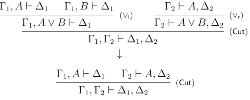
The proof of the admissibility of the cut rule, due to Gentzen, shows more than that: not only the classical sequent calculus with and without the cut rule prove the same theorems, but on top of that, we can transform, via an effective procedure, every proof in the calculus with the cut rule into a proof of the same conclusion without cuts. This procedure is described by a set of rewriting rules, which can be found for example in [Gen35]. Figure 1.2 shows the example of the (∨l) − (∧r) rewriting rule. This discovery is at the heart of what
we call the Curry-Howard correspondence: the proof of a formula ϕ can be seen as a program of type ϕ, the cut elimination steps can be seen as the execution steps of this program and the cut-free proof obtained after cut elimination corresponds to the result of the program.
Identity rules (Ax) ϕ ⊢ ϕ ⊢ ϕ, ϕ⊥ (Ax) ϕ, ϕ⊥⊢ (Ax) Γ1 ⊢ ϕ, ∆1 Γ2 ⊢ ϕ⊥, ∆2 (Cut) Γ1, Γ2 ⊢ ∆1, ∆2 Γ1, ϕ ⊢ ∆1 Γ2, ϕ⊥ ⊢ ∆2 (Cut) Γ1, Γ2 ⊢ ∆1, ∆2 Γ1 ⊢ ϕ, ∆1 Γ2, ϕ ⊢ ∆2 (Cut) Γ1, Γ2 ⊢ ∆1, ∆2 Γ1, ϕ ⊢ ∆1 Γ2 ⊢ ϕ, ∆2 (Cut) Γ1, Γ2 ⊢ ∆1, ∆2 Structural rules Γ ⊢ ∆ (Wr) Γ ⊢ ϕ, ∆ Γ ⊢ ϕ, ϕ, ∆ (Cr) Γ ⊢ ϕ, ∆ Γ ⊢ ∆1, ψ, ϕ, ∆2 (Exr) Γ ⊢ ∆1, ϕ, ψ, ∆2 Γ ⊢ ∆ (Wl) Γ, ϕ ⊢ ∆ Γ, ϕ, ϕ ⊢ ∆ (Cl) Γ, ϕ ⊢ ∆ Γ1, ψ, ϕ, Γ2 ⊢ ∆ (Exl) Γ1, ϕ, ψ, Γ2 ⊢ ∆ Logical rules Γ1 ⊢ ϕ, ∆1 Γ2 ⊢ ψ, ∆2 (∧r) Γ1, Γ2 ⊢ ϕ ∧ ψ, ∆1, ∆2 Γ ⊢ ϕ, ∆ Γ ⊢ ψ, ∆ (∧r) Γ ⊢ ϕ ∧ ψ, ∆ Γ, ϕ, ψ ⊢ ∆ (∧l) Γ, ϕ ∧ ψ ⊢ ∆ Γ1, ϕ ⊢ ∆1 Γ2, ψ ⊢ ∆2 (∨l) Γ1, Γ2, ϕ ∨ ψ ⊢ ∆1, ∆2 Γ, ϕ ⊢ ∆ Γ, ψ ⊢ ∆ (∨l) Γ, ϕ ∨ ψ ⊢ ∆ Γ ⊢ ϕ, ψ, ∆ (∨r) Γ ⊢ ϕ ∨ ψ, ∆ Γ ⊢ ϕi, ∆ (∨r) Γ ⊢ ϕ1∨ ϕ2, ∆ Γ, ϕi ⊢ ∆ (∧l) Γ, ϕ1∧ ϕ2 ⊢ ∆ Γ ⊢ ∆ (⊤l) Γ, ⊤ ⊢ ∆ (⊤r) Γ ⊢ ⊤, ∆ ⊢ ⊤ (⊤r) (⊥l) ⊥ ⊢ Γ, ⊥ ⊢ ∆ (⊥l) Γ ⊢ ∆ (⊥r) Γ ⊢ ⊥, ∆
Figure 1.1: Inference rules for LK.
Reversible and non-reversible Rules. We can classify the rules of LK in two categoris: the reversible and the non-reversible ones. A rule isreversible means that if its conclusion is provable, so are its premisses. For example, the following right rule of disjunction is reversible:
Γ ⊢ ϕ, ψ, ∆
(∨r)
Γ1, A ⊢ ∆1 Γ1, B ⊢ ∆1 (∨l) Γ1, A ∨ B ⊢ ∆1 Γ2 ⊢ A, ∆2 (∨r) Γ2 ⊢ A ∨ B, ∆2 (Cut) Γ1, Γ2 ⊢ ∆1, ∆2 ↓ Γ1, A ⊢ ∆1 Γ2 ⊢ A, ∆2 (Cut) Γ1, Γ2 ⊢ ∆1, ∆2
Figure 1.2: The (∨l) − (∧r) cut-elimination rule
Indeed, we can derive its premisse from its conclusion using the following derivation:
(Ax) Γ ⊢ ϕ⊥, ϕ (Exr),(Wr) Γ ⊢ ϕ⊥, ϕ, ψ, ∆ (Ax) Γ ⊢ ψ⊥, ψ (Exr),(Wr) Γ ⊢ ψ⊥, ϕ, ψ, ∆ (∧r) Γ ⊢ ϕ⊥∧ ψ⊥, ϕ, ψ, ∆ Γ ⊢ ϕ ∨ ψ, ∆ (Cut) Γ ⊢ ϕ, ψ, ∆
An example of a non-reversible rule is the following right rule of disjunction: Γ ⊢ ϕi, ∆
(∨r)
Γ ⊢ ϕ1∨ ϕ2, ∆
Indeed, the sequent ⊤ ⊢ ⊤ ∨ ⊥ is provable in LK, but applying the last rule (∨r), choosing
the right disjunct, leads to the sequent ⊤ ⊢ ⊥ which is not provable.
The same holds for the following right conjunction rules, where the first is reversible and the second is not:
Γ ⊢ ϕ, ∆ Γ ⊢ ψ, ∆ (∧r) Γ ⊢ ϕ ∧ ψ, ∆ Γ1 ⊢ ϕ, ∆1 Γ2 ⊢ ψ, ∆2 (∧r) Γ1, Γ2 ⊢ ϕ ∧ ψ, ∆1, ∆2
Despite this, the reversible and non-reversible versions of all the rules are inter-derivable. For instance, if the reversible version of the (∨r) is available, we can derive the non-reversible
version as follows: Γ ⊢ ϕ2, ∆ (Wr) Γ ⊢ ϕ1, ϕ2, ∆ (∨r) Γ ⊢ ϕ1∨ ϕ2, ∆ Γ ⊢ ϕ1, ∆ (Wr) Γ ⊢ ϕ2, ϕ1, ∆ (Exr) Γ ⊢ ϕ1, ϕ2, ∆ (∨r) Γ ⊢ ϕ1∨ ϕ2, ∆
Thus, if we are only concerned with provability, and if we are not interested in proofs themselves and their interaction (this will be the case for example in Part II of this thesis), it is preferable to work with a sub-system of LK, which has exactly the same expressive power as LK (that is, it proves the same sequents), but which is more suited for proof search, we call it LKrev. In this system, contraction and weakening are integrated to the rules, thus
they do not appear explicitly in the system. The cut rule being admissible, it disappears also, and we keep only the logical reversible rules.
Identity rules (Ax) Γ, ϕ ⊢ ϕ, ∆ Γ ⊢ ϕ, ϕ⊥, ∆ (Ax) Γ, ϕ, ϕ⊥⊢ ∆ (Ax) Structural rules Γ1, ψ, ϕ, Γ2 ⊢ ∆ (Exl) Γ1, ϕ, ψ, Γ2 ⊢ ∆ Γ ⊢ ∆1, ψ, ϕ, ∆2 (Exr) Γ ⊢ ∆1, ϕ, ψ, ∆2 Logical rules Γ, ϕ ⊢ ∆ Γ, ψ ⊢ ∆ (∨l) Γ, ϕ ∨ ψ ⊢ ∆ Γ ⊢ ϕ, ∆ Γ ⊢ ψ, ∆ (∧r) Γ ⊢ ϕ ∧ ψ, ∆ Γ ⊢ ϕ, ψ, ∆ (∨r) Γ ⊢ ϕ ∨ ψ, ∆ Γ, ϕ, ψ ⊢ ∆ (∧l) Γ, ϕ ∧ ψ ⊢ ∆ Γ ⊢ ∆ (⊤l) Γ, ⊤ ⊢ ∆ (⊤r) Γ ⊢ ⊤, ∆ (⊥l) Γ, ⊥ ⊢ ∆ Γ ⊢ ∆ (⊥r) Γ ⊢ ⊥, ∆
Figure 1.3: Inference rules for LKrev.
Definition 1.7. LKrev is the proof system whose rules are shown in Figure 1.3.
We can give yet another presentation of the proof system LK, this time restricting the shape of sequents. In this presentation, we allow only sequents of the form ε ⊢ Γ, where ε is the empty list, which we write simply as ⊢ Γ, and adapt the LK rules accordingly. We call the obtained proof system LKos, for one-sided LK.
Definition 1.8. LKos is the proof system whose rules are shown in Figure 1.4.
This system is equivalent to LK in the sense that if ⊢ Γ is provable in LKos then it is also
provable in LK. Conversely, if Γ ⊢ ∆ is provable in LK, then ⊢ Γ⊥, ∆ is provable in LK. The
advantage of LKos is that is has half as many rules as LK.
The proof systems for propositional classical logic presentend above are all sound and complete, this means that:
Theorem 1.2. A sequent is valid if and only if it is provable in LK (resp. LKrev, resp.
LKos).
Lafont’s critical pair. The cut elimination procedure for LK is non-deterministic in a strong sense: a proof may be reduced to two different proofs which are completely different, we say that it is non-confluent. An example of such situation is given by the following derivation, called Lafont’s critical pair. This proof will reduce either to π1 or π2 depending
Identity rules (Ax) ⊢ ϕ, ϕ⊥ ⊢ ϕ ⊥, ∆ 1 ⊢ ϕ, ∆2 (Cut) ⊢ ∆1, ∆2 Structural rules ⊢ ∆ (W) ⊢ ϕ, ∆ ⊢ ϕ, ϕ, ∆ (C) ⊢ ϕ, ∆ ⊢ ∆1, ψ, ϕ, ∆2 (Ex) ⊢ ∆1, ϕ, ψ, ∆2 Logical rules ⊢ ϕi, ∆ (∨) ⊢ ϕ1∨ ϕ2, ∆ ⊢ ϕ, ∆ ⊢ ψ, ∆ (∧) ⊢ ϕ ∧ ψ, ∆ ⊢ ϕ, ψ, ∆ (∨) ⊢ ϕ ∨ ψ, ∆ ⊢ ϕ, ∆1 ⊢ ψ, ∆2 (∧) ⊢ ϕ ∧ ψ, ∆1, ∆2 (⊤) ⊢ ⊤, ∆ ⊢ ⊤ (⊤) ⊢ ∆ (⊥) ⊢ ⊥, ∆
Figure 1.4: Inference rules for LKos.
on the direction we choose to reduce cuts.
π1 ⊢ Γ (W) ⊢ Γ, Γ (C) ⊢ Γ ⋆ ← π1 ⊢ Γ (W) ⊢ ϕ⊥, Γ π2 ⊢ Γ (W) ⊢ ϕ, Γ (Cut) ⊢ Γ, Γ (C) ⊢ Γ →⋆ π2 ⊢ Γ (W) ⊢ Γ, Γ (C) ⊢ Γ
If we think about cut elimination as a computational process transforming a proof into a result, this last observation is problematic since it means that a computation does not give a unique result. One way to get rid of such critical pairs and to retrieve more determinism is to control the use of structural rules. This is one of the innovations of linear logic, which we introduce in the next section.
1.3
Linear Logic
In LKos, some rules require identical contexts in all their premises, which they supperpose
in the conclusion sequent, we call them additive rules. This is the case of the following rules for instance:
⊢ ϕ, ∆ ⊢ ψ, ∆ (∧) ⊢ ϕ ∧ ψ, ∆ ⊢ ϕi, ∆ (∨) ⊢ ϕ1∨ ϕ2, ∆