This work is supported by the CNPq - FNRS, the Belgian Science Policy (IAP P6/21) and the Walloon Region.
The Perturbation Finite Element Method for Magnetic Modeling of a
Loudspeaker
M. V. Ferreira da Luz1, P. Dular2, R. V. Sabariego2 and P. Kuo-Peng1 1
GRUCAD/EEL/UFSC, Po. Box 476, 88040-970, Florianópolis, Santa Catarina, Brazil. 2
Dept. of Electrical Engineering and Computer Science, F.N.R.S., University of Liège, Belgium. E-mail: mauricio@grucad.ufsc.br
Abstract ⎯ This paper shows that the application of a perturbation finite element method can provide a useful alternative to correct the equivalent magnetic circuits used to model loudspeakers. A ring magnet design of a loudspeaker is modeled by means of an axisymmetric magnetic vector potential formulation. The effects of geometry variations on its performances are analyzed. The perturbation solution allows further adapting and refining the equivalent magnetic circuit model of the loudspeaker to each possible variation. Results will be compared with the classical finite element solution.
I. INTRODUCTION
A loudspeaker is an electromechanical transducer which converts electrical energy to mechanical work in the form of acoustic power [1] [2]. Loudspeakers can be modeled for instance by equivalent magnetic circuits or the finite element method. However, for any variation of geometrical or physical characteristics a new complete finite element (FE) computation must be performed or a new equivalent circuit must be studied.
(a) (b)
(c) Fig. 1. Ring magnet design: 3D image (a) and transversal cut of the loudspeaker magnetic circuit (b). The transversal cut of the loudspeaker
magnetic circuit with low leakage flux design (c).
The perturbation finite element method is an excellent tool to deal with this kind of geometrical variations. Benefits are particularly aimed for allowing different problem-adapted meshes and for computational efficiency due to the reduce size of each sub-problem [3]. In this work a perturbation method is used in the magnetic design of a loudspeaker and the effects of geometry variations on its performance are analyzed. This approach allows to straightforwardly correct the equivalent circuit for each geometry variation performed.
In general, the magnetic circuit of a permanent magnet (PM) loudspeaker has a ring magnet design or a cylinder magnet design. The ring magnet design shown in Fig. 1a and Fig. 1b has the magnet material outside the voice coil, so the magnetic circuit efficiency is much lower, only
35-50% of the total flux is used [2]. However, such a ring design allows a larger magnet area and hence lower remanent magnetic flux density materials can be used.
Ferrite magnet loudspeakers have low circuit efficiency but still give acceptable solutions because of the low cost ferrite magnet. This magnet compensates for two major disadvantages [2]: (i) the soft iron parts for the ferrite ring design are large and expensive; (ii) the high leakage flux is difficult to tolerate in some application environments, e.g. in automotive dashboard locations.
For the ring design, a circuit modification can be made (Fig. 1c) to cancel the leakage flux due to the second ring magnet. This is an effective functional solution, although the savings made are questionable.
II. REFERENCE AND MODIFIED PROBLEMS A. Reference problem and its strong formulation
A magnetostatic problem p is defined in a bounded domain Ωp, with boundary ∂Ωp=Γh,p∪Γb,p, of the two or three-dimensional Euclidean space.
A problem, defined with subscript p = 1, is first considered. Its equations and material relations in Ω1 are:
1 1
curlh = j , divb1=0, b1=μ1h1+br1, (1a-b-c)
with boundary conditions (BCs) and interface conditions (ICs) ,1 1 0 h Γ × = n h , ,1 1 . 0 b Γ = n b , (1d-e) 1 , su 1]1 [n×h γ = j , [n .b1]γ1 =bsu,1, (1f-g)
where h is the magnetic field, b is the magnetic flux density, j is the electric current density, μ is the magnetic permeability and n is the unit normal exterior to Ω. The notation [ . ] = . |γ+ − . |γ- expresses the discontinuity of a quantity through any interface γ (of both sides γ+ and γ−
), which is allowed to be non-zero; the associated surface fields jsu,1 and bsu,1 are usually unknown, i.e., parts of the solution [3]. It is intended to solve successive problems, the solutions of which being added to get the solution of a complete problem. At the first step, a simplified problem p = 1 is solved either analytically or with the FE method. Its solution is called reference or source solution. In both cases, it is based on particular assumptions that aim to simplify its solving but that are to be further corrected. B. Modified problem defining perturbation
A modification of the problem p = 1 leads to a perturbation of its solution. This can result from the change of properties of existing materials or from the addition or suppression of materials, which actually also amounts to
changing some material properties [3]. Both large and small perturbations are considered. The governing equations and relations in other domains Ω2 and Ω3, i.e. successive modified forms of Ω1 (Fig. 2a), and the BCs and ICs, are still on the form (1) with all the involved relative quantities to the new solution and the involved relative boundaries to Ω2 and Ω3. The domain Ω2 considers the perturbation due to the variation of the magnetic circuit in Ω1. The domain Ω3, shown in Fig. 2b, considers the perturbation due to the inclusion of another ferrite PM (PM2) in Ω2. We have chosen to analyze these perturbations separately to quantify their individual effect on the equivalent circuit used to model the loudspeakers.
The solution of the complete problem can be thus decomposed in three parts: the reference solution and two perturbations of this one. These quantities are given by
3 2 1 h h h h= + + , b=b1+b2+b3, (2a-b) 3 2 1 r r r r b b b b = + + , j=j1+ j2+ j3, (2c-d) 3 , 2 , 1 , su su su su j j j j = + + , bsu =bsu,1+bsu,2+bsu,3. (2e-f) Subtracting each equation of (1) from its counterpart in the so-modified problem, the perturbation equations that define the problem p = 2, are
2 2
curlh = j , divb2=0, b2=μ2h2+br2+bs,2, (3a-b-c) ,2 2 0 h Γ × = n h , ,2 2 . 0 b Γ = n b , (3d-e) 2 , su 2] 2 [n×h γ = j , [n .b2]γ2 =bsu,2, (3f-g) and the perturbation equations that define the problem p =
3, are
3
3 j
h =
curl , divb3=0, b3=μ3h3+br3+bs,3, (4a-b-c) 0 3 , 3 = × Γ h h n , . 0 3 , 3Γb = b n , (4d-e) 3 , 3] 3 [n×h γ = jsu , [n .b3]γ3 =bsu,3, (4f-g) where the so-defined volume sources bsu,2 and bsu,3 are
obtained from the reference solution (either analytical or numerical) as 1 1 2 2 , ( )h bs = μ −μ and bs,3=(μ3−μ2)(h1+h2). (5a-b) The perturbation fields are still governed by the Maxwell equations in their classical forms (3a-b) and (4a-b). However, their associated material relations now include the additional sources (3c) and (4c), that only acts in the modified regions.
III. PERTURBATION FINITE ELEMENT METHOD AND APPLICATION
A ring magnet design of the loudspeaker is considered as a test case. The solution domain is an axial cross-section of the axisymmetric geometry (Fig. 2). A reference solution is first calculated (Fig. 2a) with a ferrite PM (PM1) as excitation. In this case, a transformation air layer is used with infinite boundaries around the magnetic circuit to prevent errors due to the truncation of the computational domain. The reference solution serves then as a source for a perturbation problem (Fig. 2b) defined with another
ferrite PM (PM2) as excitation. The complete solution domain is shown in Fig. 2c.
The solutions are transferred from one problem to the other through projections of the source fields between the independent meshes [4]. Solving the perturbation problem instead of the complete one enables to avoid operations already performed in the reference problem.
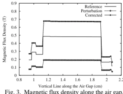
Fig. 3 shows the magnetic flux density along a vertical line in the air gap. It can be observed that with two PM’s the leakage decreases and the magnetic flux density increases in the air gap.
(a) + (b) =
(c)
Fig. 2. The solution domain of a ring magnet design: reference solution (field lines) with PM1 (a), perturbation solution with PM2 and with the
magnetic circuit modified (b), complete (corrected) solution (c).
0 0.1 0.2 0.3 0.4 0.5 0.6 0.7 0.8 0.9 0.8 1 1.2 1.4 1.6 1.8 2 2.2
Magnetic Flux Density (T)
Vertical Line along the Air Gap (cm) Reference Perturbation Corrected
Fig. 3. Magnetic flux density along the air gap.
The perturbation solution allows adapting and refining the equivalent magnetic circuit model of a loudspeaker, pointing out the significance of each variation.
The modifications in the equivalent circuit will be analyzed when adding first an iron part and second a ferrite PM to the loudspeaker structure. Results will be compared with the classical finite element solution.
The definition of the sources of the perturbation problem and the corrections of the equivalent magnetic circuit of loudspeaker will be detailed in the extended paper.
REFERENCES
[1] M. Jufer, Transducteurs électromécaniques, Traité d'Électricité, Vol. IX, Presses Polytechniques Romandes, Lausanne, 1985.
[2] R. J. Parker, Advances in permanent magnetism, John Wiley & Sons, 1989.
[3] P. Dular and R. V. Sabariego, “A perturbation finite element method for modeling moving conductive and magnetic regions without remeshing,” COMPEL International Journal for Computation and
Mathematics in Electrical and Electronic Engineering, vol. 26, no.
3, pp. 700-711, 2007.
[4] P. Dular and R. V. Sabariego, “A perturbation method for computation field distortions due to conductive regions with h-conform magnetodynamic finite element formulations”, IEEE Trans.