• Aucun résultat trouvé

An Efficient Representation Format for Fuzzy Intervals Based on Symmetric Membership Functions

N/A
N/A
Protected

Academic year: 2021

Partager "An Efficient Representation Format for Fuzzy Intervals Based on Symmetric Membership Functions"

Copied!
22
0
0

Texte intégral

(1)

An efficient representation format for fuzzy intervals based on

symmetric membership functions

MANUEL MARIN, University of Li`ege

DAVID DEFOUR, University of Perpignan Via Domitia

FEDERICO MILANO, University College Dublin

This paper addresses the execution cost of arithmetic operations with a focus on fuzzy arithmetic. Thanks to an appropriate representation format for fuzzy intervals, we show that it is possible to halve the number of operations and divide by 2 to 8 the memory requirements compared to conventional solutions. In addition, we demonstrate the benefit of some hardware features encountered in today’s accelerators (GPU) such as static rounding, memory usage, instruction level parallelism (ILP) and thread-level parallelism (TLP). We then describe a library of fuzzy arithmetic operations written in CUDA and C++. The library is evaluated against traditional approaches using compute-bound and memory-bound benchmarks on Nvidia GPUs, with an observed performance gain of 2 to 20.

CCS Concepts: rMathematics of computing → Interval arithmetic; rComputer systems organiza-tion → Multicore architectures;

Additional Key Words and Phrases: Fuzzy intervals, Graphic Processing Units, Midpoint-radius, Lower-upper

ACM Reference Format:

Manuel Marin, David Defour and Federico Milano, 2015. An efficient representation format for fuzzy inter-vals based on symmetric membership functions. ACM Trans. Math. Softw. V, N, Article A (January YYYY), 22 pages.

DOI: http://dx.doi.org/10.1145/0000000.0000000

1. INTRODUCTION

The cost of operations involving fuzzy arithmetic is an order of magnitude higher than classic interval arithmetic which is itself an order of magnitude higher than oper-ations on floating-point numbers. Therefore it is highly desirable to design efficient implementations of fuzzy interval arithmetic. However, interval arithmetic libraries are designed and optimized for interval operations and do not exploit specificity of fuzzy intervals. Similarly fuzzy arithmetic libraries that internally rely on existing interval arithmetic implementations do not exploit hardware specificity. This leads to sub-optimal implementations. In this paper, we consider every layer involved in the design of an efficient fuzzy interval arithmetic implementation.

Fuzzy interval arithmetic is a relevant tool for dealing with uncertainty in numer-ical data [Hanss 2010]. Recent examples of fuzzy arithmetic applications are found in group decision making [Xia et al. 2013; Baleˇzentis and Zeng 2013], medical diag-nosis [C¸ elik and Yamak 2013], reliability analysis [Sriramdas et al. 2014; Shaw and Roy 2013], geology [Park et al. 2012], model validation [Haag et al. 2012], and power systems [Marin et al. 2014]. In the classic approach to interval arithmetic, a region is

Author’s addresses: M. Marin, Montefiore Institute, University of Li`ege; D. Defour, DALI-LIRMM, Univer-sity of Perpignan Via Domitia; F. Milano, School of Electrical and Electronic Engineering, UniverUniver-sity College Dublin.

Permission to make digital or hard copies of all or part of this work for personal or classroom use is granted without fee provided that copies are not made or distributed for profit or commercial advantage and that copies bear this notice and the full citation on the first page. Copyrights for components of this work owned by others than ACM must be honored. Abstracting with credit is permitted. To copy otherwise, or repub-lish, to post on servers or to redistribute to lists, requires prior specific permission and/or a fee. Request permissions from permissions@acm.org.

c

YYYY ACM. 0098-3500/YYYY/01-ARTA $15.00 DOI: http://dx.doi.org/10.1145/0000000.0000000

(2)

defined to which the value of a variable is expected to belong. This allows modelling uncertainty if the information about the bounds is available, e.g., “the speed is between 20 and 50 km/h”. However, if the information is more ambiguous and imprecise, e.g., “the speed is about 30 km/h”, then the classic approach fails and the fuzzy interval approach can be more appropriate [Siler and Buckley 2005].

Fuzzy intervals are characterized by a membership function, which assigns to each number in the real domain a degree of membership within the fuzzy interval. In re-turn, the membership function is characterized by its shape, with some standards such as the trapezoidal form and the Gaussian bell [Cort´es-Carmona et al. 2010; Shaw and Roy 2013]. Fuzzy interval operations are defined in compliance with Zadeh’s exten-sion principle [Zadeh 1975]. This paper considers the α-cut approach, which splits the fuzzy interval by degree of membership into a finite set of ‘crisp’ intervals [Dubois and Prade 1978]. Then, fuzzy arithmetic operations can be carried out by using crisp inter-val arithmetic in any of its representation formats, e.g., lower-upper, midpoint-radius or even lower-diameter [Moore 1966; Neumaier 1990]. Efficient implementations of crisp interval arithmetic are nowadays provided by several software packages [Revol and Rouillier 2001; Br¨onnimann et al. 2006; Goualard 2006]. In addition, one can find dedicated implementations of fuzzy arithmetic in the related literature [Anile et al. 1995; Kolarovic 2013; Gagolewski 2015]. However, one of the main issues with these implementations is that they rely on the lower-upper representation format. As re-sult, applications cannot take advantage of specific information about the membership function, such as symmetry, which can be exploited by other formats, such as midpoint-radius.

This paper presents a novel implementation of fuzzy interval arithmetic that specif-ically considers the case of symmetric membership function. The implementation is tuned to exploit hardware capabilities of Graphics Processing Units (GPUs), while keeping compatibility with traditional CPU architectures. The main contributions of the paper are detailed below:

— Dedicated representation format for symmetric fuzzy intervals. We explore the case of symmetric membership function and propose a novel representation for-mat based on the midpoint-radius approach. Whereas this forfor-mat restricts the spec-trum of fuzzy intervals that can be processed to the symmetric case, we demonstrate that it considerably boosts performance of basic fuzzy applications. This is due to the impact on the the amount of operations and memory required that is divided by min-imum two compared to the lower-upper approach. In addition, we propose a second format based on the midpoint-increment approach, which improves the accuracy of the previous while maintaining or even reducing the number of operations involved. — Fuzzy arithmetic library implementation. We describe the implementation of the above formats and the traditional lower-upper format into a library of fuzzy arith-metic operations, available online at https://github.com/mmarin-upvd/fuzzy-gpu/. Implementation aspects such as static rounding, memory requirements, instruction-level parallelism (ILP) and thread-instruction-level parallelism (TLP) are thoroughly consid-ered. We also evaluate the performance of our library on two classes of applications: compute-bound and memory-bound applications.

The remainder of the paper is organized as follows: in Section 2, the mathematical framework of fuzzy interval arithmetic is presented. Section 3 describes the proposed representation formats for symmetric fuzzy intervals. The implementation of these formats into a fuzzy arithmetic library is detailed in Section 4. Section 5 evaluates performance of the library on GPU. Finally, Section 6 draws conclusions and outlines future work.

(3)

Table I. Notation for fuzzy interval arithmetic and rounding Symbol Definition x Scalar. [x] Interval. [˜x] Fuzzy interval. x Lower bound of [x]. x Upper bound of [x]. ˇ x Midpoint of [x]; kernel of [˜x]. ρx Radius of [x]. µ(·) Membership function. [xi] α-cut of level i of [˜x]. ρx,i Radius of [xi].

δx,i Radius increment associated to [xi]. △(·) Rounding upwards.†

▽(·) Rounding downwards.† (·) Rounding to nearest.† ǫ Relative rounding error.

η Smallest representable (unnormalized) floating-point positive number. †The rounding attribute applies on all the operations included within the parenthe-ses.

2. MATHEMATICAL BACKGROUND

In order to support the discussion of following sections, the basic concepts of inter-val arithmetic and α-cut fuzzy arithmetic are outlined next. Table I summarizes the notation used throughout the remainder of the paper.

2.1. Interval arithmetic

Intervals are defined as convex sets of real numbers. We assume that, given a real number and an interval, the real number either belongs to the interval or not. In this way, each element in the interval is considered equally possible (and each element outside the interval, equally impossible).

2.1.1. Interval representation.Intervals can be represented in several formats, e.g., through lower and upper bounds, midpoint and radius, or lower bound and diameter. This paper considers the first two alternatives, as follows.

Definition2.1 (Lower-upper representation). Let [x] be an interval defined by [x] = {x ∈ R : x ≤ x ≤ x},

where x, x ∈ R, x ≤ x. We write [x] = [x, x].

Definition2.2 (Midpoint-radius representation). Let [x] be an interval defined by [x] = {x ∈ R : |x − ˇx| ≤ ρx},

where ˇx, ρx∈ R, ρx≥ 0. We write [x] = hˇx, ρxi.

2.1.2. Interval operations and rounding.Interval arithmetic operations are defined by extending operations on real numbers to intervals. The basic property of inclusion isotonocityis assumed, as follows.

Definition2.3 (Inclusion isotonicity). Let ◦ be a basic arithmetic operation, i.e., ◦ ∈ {+, −, ·, /}, [x] and [y] intervals. If

x ◦ y ⊆ [x] ◦ [y] , ∀ x ∈ [x] , ∀ y ∈ [y] , then ◦ is said to be inclusion isotone.

(4)

Inclusion isotonicity ensures that no possible values are “left behind” when perform-ing interval operations. To respect this property, interval arithmetic implementations have to cope with floating-point rounding errors.

The IEEE-754 Standard for floating-point computation establishes that the follow-ing three roundfollow-ing attributes must be available: roundfollow-ing upwards (towards infinity), rounding downwards (towards minus infinity), and rounding to nearest [Zuras et al. 2008]. The IEEE-754 Standard also defines the relative rounding error and the small-est representable (unnormalized) floating-point number, the latter being associated with the underflow error [Rump 1999; Higham 2002] (see Table I for notation details). In the lower-upper representation, isotonicity implies rounding downwards when computing the lower bounds, and upwards when computing the upper bounds [Dubois and Prade 1978]. The interval operations for the lower-upper representation are de-fined below.

Definition2.4 (Lower-upper interval operations). Let [x] = [x, x] and [y] = [y, y], where x, x, y, y are floating-point numbers. Let ▽(·) and △(·) be the rounding attributes towards minus infinity and plus infinity, respectively. Then

[x] + [y] = [▽(x + y), △(x + y)], [x] − [y] = [▽(x − y), △(x − y)],

[x] · [y] = [▽(min(xy, xy, xy, xy)), △(max(xy, xy, xy, xy))], 1 [y] =  ▽ 1 y  , △ 1 y  , 0 /∈ [y] .

In the case of the midpoint-radius representation, in addition to adequate rounding, isotonocity requires adding to the radius the error due to midpoint rounding [Rump 1999]. The interval operations for the midpoint-radius representation are defined be-low.

Definition2.5 (Midpoint-radius interval operations). Let [x] = hˇx, ρxi and

[y] = hˇy, ρyi, where ˇx, ρx, ˇy, ρy are floating-point numbers. Let (·) and △(·) be

the rounding attributes to nearest and towards plus infinity, respectively. Let ǫ be the relative rounding error, ǫ′ = 1

2ǫ and η be the smallest representable (unnormalized)

floating-point positive number. Then [x] ± [y] = hz, △(ǫ′|z| + ρ

x+ ρy)i, z = (ˇx ± ˇy), (2a)

[x] · [y] = hz, △(η + ǫ′|z| + (|ˇx| + ρ

x)ρy+ |ˇy|ρx)i, z = (ˇxˇy), (2b)

1 [y] =  z, △  η + ǫ′|z| + −ρy |ˇy|(ρy− |ˇy|  , z =  1 ˇ y  , 0 /∈ [y] . (2c) It is worth noting that both equations (2b) and (2c) introduce a bounded overesti-mation over the lower-upper format definition. In the case of the multiplication, the overestimation is bounded by a factor of 1.5 [Rump 1999].

The impact of rounding on performance depends on the computing architecture. For example, for most CPU architectures, the rounding attribute is a processor ‘mode’, and thus changes in rounding mode cause the entire instruction pipeline to be flushed.

2.1.3. The dependency problem.The so-called dependency problem causes overestima-tion in interval computaoverestima-tions where the same variable occurs more than once. Since all the instances of the same variable are taken independently by the rules of inter-val arithmetic, the radius of the result might be expanded to unrealistic inter-values. For

(5)

example, consider the function, f (x) = x2− 1, where x ∈ [−1, 1]. Then, f (x) ∈ [−1, 0].

However, using interval arithmetic, f ([−1, 1]) = [−1, 1] · [−1, 1] − 1 = [−2, 0].

This can become a major issue to the application of interval arithmetic to real-world problems, especially to non-linear ones. Accordingly, specific measures have to be taken to preserve the relevance of the results.

2.2. Fuzzy interval arithmetic

Fuzzy intervals are defined as fuzzy sets of real numbers. Given a number and a fuzzy interval, the number belongs to the fuzzy interval with a certain degree of member-ship. Elements with a higher degree are considered more possible than elements with lower degrees. This is the main feature that distinguishes fuzzy intervals from regular intervals.

2.2.1. Fuzzy interval representation.Fuzzy intervals are characterized by a membership function. This paper considers continuous membership functions with a single maxi-mum point. The definition of membership function is as follows.

Definition2.6 (Membership function). Let µ(·) : R → [0, 1] be a continuous function. Let x, ˇx, x ∈ R, such that x ≤ ˇx ≤ x, and:

µ(ˇx) = 1, µ(x1) < µ(x2), ∀ x1, x2∈ [x, ˇx], x1< x2,

µ(x1) > µ(x2), ∀ x1, x2∈ [ˇx, x], x1< x2,

µ(x) = 0, ∀ x /∈ [x, x].

Then, µ(·) is called a membership function. In addition, the element ˇx is called kernel and the interval [x, x] is called support.

In other words, the membership function is strictly increasing until reaching its maximum, and then strictly decreasing. The formal definition of fuzzy interval is given below.

Definition2.7 (Fuzzy interval). Let µ(·) be a membership function. Then, the set [˜x] = {(x, µ(x)) : x ∈ R},

is called a fuzzy interval.

According to Definition 2.7, a fuzzy interval is a set of ordered pairs, each composed of a real number and a degree of membership, the latter given by a membership func-tion. Figure 1 shows an example of fuzzy interval.

2.2.2. Fuzzy interval operations: theα-cut approach.Fuzzy interval operations are defined by extending operations on real numbers to fuzzy intervals. In [Zadeh 1975], the au-thor presents a principle to extend computations to fuzzy sets that has become widely accepted. The definition regarding arithmetic operations is given below.

Definition2.8 (Zadeh’s extension principle). Let ◦ ∈ {+, −, ·, /}, and [˜x] , [˜y] , [˜z], fuzzy intervals, such that [˜z] = [˜x] ◦ [˜y]. Let µx, µy, µz, be the membership functions

of each. Then

µz(z) = sup

z=x◦ymin{µx(x), µy(y)}.

In this article we rely on the α-cut approach to implement Zadeh’s principle. This approach consists in splitting the fuzzy intervals into finite sets of crisp intervals char-acterized by given membership degree [Dubois and Prade 1978]. These intervals are called α-cuts. Each uncertainty level, or α-level, is assigned a membership degree,

(6)

x µ(x) ˇ x 1 0.6 0.3

Fig. 1. Fuzzy interval, membership function andα-cuts.

αi ∈ [0, 1], such that α1> . . . > αN, where N is the number of levels. For each level i,

the corresponding α-cut contains all the real numbers having membership degree at least αi. The formal definition of α-cut is the following:

Definition2.9 (α-cut). Let [˜x] be a fuzzy interval with membership function µ(·). Let N ∈ N, i ∈ {1, . . . , N }, and αi ∈ [0, 1]. Then

[xi] = {x ∈ R : µ(x) ≥ αi},

is called an α-cut (of level i) of the fuzzy interval [˜x].

The assumptions made on the membership function (see Definition 2.6) allow the α-cuts to become well-defined intervals, as seen in Fig. 1. Once the α-cuts are obtained for each operand, the α-cut concept defined below may be applied.

Definition2.10 (α-cut concept). Let ◦ ∈ {+, −, ·, /}, and [˜x] , [˜y] , [˜z], fuzzy intervals, such that [˜z] = [˜x] ◦ [˜y]. Let [xi] , [yi] , [zi], be the α-cuts of level i of each. Then

[zi] = [xi] ◦ [yi] .

The above defines a way to perform fuzzy operations, where α-cuts of the result are computed via the corresponding interval operation between α-cuts of the operands. 3. PROPOSED FUZZY ARITHMETIC IMPLEMENTATION

This section presents two novel approaches to implement fuzzy interval arithmetic based on the midpoint-radius format.

3.1. Midpoint-radius format

The shape of the membership function is a crucial aspect in fuzzy modelling [Boukez-zoula et al. 2014]. This section considers a membership function symmetric with re-spect to a vertical axis, which is of particular relevance in several fuzzy arithmetic applications [Chang and Wu 1995; Mendel and Wu 2006]. For symmetric membership functions, all α-cuts are centered on the kernel, which leads to relevant properties that are exploited by the proposed implementation. The definition of a symmetric fuzzy in-terval is given below.

Definition3.1 (Symmetric fuzzy interval). Let [˜x] be a fuzzy interval with member-ship function µ(·) and kernel ˇx. If µ(·) is symmetric around ˇx, i.e.,

(7)

ALGORITHM 1:Symmetric fuzzy multiplication in the midpoint-radius format (see Table I for notation details)

Input: Symmetric fuzzy operands [˜x] and [˜y]. Output: Symmetric fuzzy result [˜z] = [˜x] · [˜y]. kernel: ˇz = (ˇxˇy);

fori in 1, . . . , N do

radius: ρz,i= △(η +12ǫ|ˇz| + (|ˇx| + ρx,i)ρy,i+ |ˇy|ρx,i);

end

then [˜x] is called a symmetric fuzzy interval.

Although symmetry is immaterial for the lower-upper interval representation, it is relevant for the midpoint-radius representation, as it is stated by the following propo-sition.

PROPOSITION 3.2. Let [˜x] be a symmetric fuzzy interval with kernel ˇx. Let N ∈ N, i ∈ {1, . . . , N }, and [xi] = hˇxi, ρx,ii, an α-cut. Then,

x] is symmetric ⇐⇒ ˇxi = ˇx, ∀ i ∈ {1, . . . , N }.

PROOF. See Appendix 6.

The above result can be graphically seen in Fig. 1, where the fuzzy interval is sym-metric. Note how all the α-cuts are centered on the kernel. The property of symmetry is also preserved by basic fuzzy arithmetic operations, as stated by the following theo-rem.

THEOREM 3.3. Let [˜x] and [˜y] be fuzzy intervals, ◦ ∈ {+, −, ·, /}. If [˜x] and [˜y] are symmetric, then[˜z] = [˜x] ◦ [˜y] is also symmetric.

PROOF. See Appendix 6.

Proposition 3.2 and Theorem 3.3 are applied next to propose an efficient representa-tion format for symmetric fuzzy intervals. Fuzzy intervals are stored in two elements: (i) the kernel (or midpoint, common to all α-cuts) and (ii) a set of radii (one per α-cut). Fuzzy operations are also solved in two steps: (i) the computation of the kernel, and (ii) the computation of the individual radius of each α-cut. For the sake of example, Algorithm 1 illustrates the fuzzy multiplication. As shown in Section 5, this format allows saving both bandwidth and execution time when performing fuzzy operations on symmetric fuzzy intervals.

3.2. Midpoint-increment format

Another relevant property of fuzzy intervals is that every α-cut is fully contained within any lower level α-cut [Fortin et al. 2008]. This is an immediate consequence of the membership function being strictly increasing until reaching its maximum, and then strictly decreasing.

PROPOSITION 3.4. Let [˜x] be a fuzzy interval, N ∈ N, i, j ∈ {1, . . . , N }, and [xi] , [xj],

α-cuts. Then

αi > αj =⇒ [xi] ⊂ [xj] .

PROOF. See Appendix 6.

The result above is applied next to propose a representation format for symmet-ric fuzzy intervals. The fuzzy intervals are stored in two elements: (i) the kernel (or midpoint, common to all α-cuts), and (ii) a set of radius increments (one per α-cut).

(8)

ALGORITHM 2:Symmetric fuzzy addition and subtraction in the midpoint-increment format (see Table I for notation details)

Input: Symmetric fuzzy operands [˜x] and [˜y]. Output: Symmetric fuzzy result [˜z] = [˜x] ± [˜y]. kernel: ˇz = (ˇx ± ˇy);

first increment: δz,1= △(12ǫ|ˇz| + δx,1+ δy,1);

fori in 2, . . . , N do

increment: δz,i= △(δx,i+ δy,i);

end

The latter correspond to the difference between the radii of two consecutive α-cuts, as defined below.

Definition3.5 (Radius increments). Let [˜x] be a fuzzy interval, N ∈ N and i ∈ {1, . . . , N }. Let {α1, . . . , αN} ∈ [0, 1], such that α1> . . . > αN. Let [x1] , . . . , [xN], be

α-cuts and ρx,1, . . . , ρx,N, their respective radii. The numbers, δx,1, . . . , δx,N, defined as:

δx,i=ρx,i− ρx,i−1 if 2 ≤ i ≤ N,

ρx,1 if i = 1,

are called radius increments. The set of radius increments can be computed with the iterated difference function (diff ) available in numerical packages such as Matlab or Numpy.

From the above definition, it is transparent that any radius of level i can be com-puted as a sum of increments:

ρx,i= i

X

k=1

δx,k.

The purpose of this format is to increase the accuracy of fuzzy computations. As the increments are, by definition, smaller than the radii, the rounding errors associated with increments computation are also smaller. This concept is further developed in Section 3.3.

Algorithms 2, 3 and 4 show how to compute the addition, subtraction, multiplication and inversion. Note that the number of floating-point operations needed by this format is not increased compared to midpoint-radius. In fact, addition and subtraction require one fewer operation per α-cut than the midpoint-radius. Multiplication and inversion require the same amount of operations per α-cut, provided that the α-cuts are treated sequentially (such that certain computations associated to a given α-level can be re-used in the following level).

In Algorithms 2, 3 and 4, the kernel’s rounding error is added only to the first in-crement, so one operation per α-cut is saved. In the case of the multiplication and inversion, i has to be increased sequentially. Variables t(·) are introduced to serve as accumulators. In the multiplication, these accumulators store the maximum (absolute) value of two α-cuts, one in each operand, one level apart from each other. Only one op-eration is needed to update the accumulator at each α-level. Interestingly, these accu-mulators allow for a quite transparent calculation of the increment. The same amount of operations are needed as in computing the full radius using the midpoint-radius format.

(9)

ALGORITHM 3:Symmetric fuzzy multiplication in the midpoint-increment format (see Table I for notation details)

Input: Symmetric fuzzy operands [˜x] and [˜y]. Output: Symmetric fuzzy result [˜z] = [˜x] · [˜y]. kernel: ˇz = (ˇxˇy);

accumulator in [˜x]: tx,1= △(|ˇx| + δx,i);

accumulator in [˜y]: ty,1= △(|ˇy|);

first inc.: δz,1= △(η + 12ǫ|ˇz| + tx,1δy,1+ ty,1δx,1);

fori in 2, . . . , N do

accumulator in [˜x]: tx,i= △(tx,i−1+ δx,i);

accumulator in [˜y]: ty,i= △(ty,i−1+ δy,i);

increment: δz,i= △(η +12ǫ|ˇz| + tx,iδy,i+ ty,iδx,i);

end

ALGORITHM 4:Symmetric fuzzy inversion in the midpoint-increment format (see Table I for notation details)

Input: Symmetric fuzzy operand [˜y]. Output: Symmetric fuzzy result [˜z] = 1/ [˜y]. kernel: ˇz = (1/ˇy);

accumulator: ty,1= |ˇy|;

first increment: δz,1= △(η +12ǫ|ˇz| + (−δy,1)/(ty,1(δy,1− ty,1));

fori in 2, . . . , N do

accumulator: ty,i= △(ty,i−1− δy,i−1);

increment: δz,i= △(η +12ǫ|ˇz| + (−δy,i)/(ty,i(δy,i− ty,i));

end

3.3. Error analysis

This section compares the accuracy of radius computations in both proposed formats. The main operation involved in this kind of computation is the rounded floating-point addition. The following result, which concerns the error associated to floating-point summation algorithms, is useful for the analysis that is discussed later in this section. THEOREM3.6 (BOUND FOR THE ABSOLUTE SUMMATION ERROR[HIGHAM2002]). Let x1, . . . , xn ∈ R and Sn = P

n

i=1xi. Let ˆSn be an approximation to Sn computed by a summation algorithm, which performs exactlyn − 1 floating-point additions. Let

ˆ

T1, . . . , ˆTn−1, be then − 1 partial sums computed by such algorithm. Then,

En:= Sn− ˆSn ≤ ǫ n−1 X i=1 Tˆi ,

whereǫ is the relative rounding error. PROOF. See [Higham 2002].

Hence, the absolute error introduced by a floating-point summation algorithm is no greater than the relative rounding error, multiplied by the sum of magnitudes of all the intermediate sums.

Theorem 3.6 is used for proving that the midpoint-increment format improves the accuracy of basic fuzzy computations, compared to midpoint-radius. The result pre-sented below is a direct consequence of the increments being smaller in magnitude than the radii.

(10)

THEOREM 3.7. Let ◦ ∈ {+, −, ·, /} and [˜x] , [˜y] , [˜z], be fuzzy intervals, such that [˜z] = [˜x] ◦ [˜y]. Let [zi] be the α-cut of level i of [˜z], and ρz,i, the radius of[zi]. Let E(rad)(·) andE(inc)(·) return the maximum absolute error in the radius and midpoint-increment formats, respectively. Then,

E(inc)(ρz,i) < E(rad)(ρz,i), ∀ i ≥ 2.

PROOF. See Appendix 6.

Theorem 3.7 allows concluding that the gain in accuracy is driven ultimately by the fact that the radius at any α-level is always greater than the one at the previous level. This, in turn, is a consequence of the monotonicity of the membership function. In the midpoint-increment format, the smallest radius is computed first, and then the others by simply adding the increments. In other words, large values are broken down into smaller ones, prior to perform fuzzy computations. As these computations are composed mainly of floating-point additions, the strategy reduces rounding error in absolute value.

It can be shown that the result holds for any summation algorithm chosen to com-pute the increments and the radii, as long as it is the same for both. However, this proof is omitted for sake of brevity. The accuracy gain can also be quantified. It de-pends on several factors, e.g., the considered summation algorithm (i.e., the order of the operations); the ratio of increment to radius at different α-levels; the “precision” of the intervals (i.e., the ratio of midpoint to radius); and the relative rounding error ǫ. 4. GPU IMPLEMENTATION

The proposed midpoint-radius and the traditional lower-upper format are imple-mented into a library of fuzzy arithmetic operations written in CUDA and C++, avail-able online at https://github.com/mmarin-upvd/fuzzy-gpu/. The implementation of the midpoint-increment format is planned as future work.

The library is designed to adapt itself to the underlying architecture, whether this is CPU or GPU. It relies on a rounded arithmetic class which defines basic arithmetic operations in different rounding modes. In the case of CPU, this is implemented by updating the rounding mode before the operation, and reestablishing it afterwards. In the case of GPU, it is achieved by calling the dedicated machine instruction with the specific rounding attribute.

The rounded arithmetic class is used to implement an interval class in the lower-upper format, which is subsequently used to implement a fuzzy interval class in the lower-upper format. The above is the traditional approach. Now, in the case of the midpoint-radius approach, we do not provide the intermediate interval class as we want to exploit the results from Theorem 3.3 in the previous section. This result es-tablishes that midpoint-radius fuzzy intervals are better handled as a whole entity, where the midpoint is shared by all the α-cuts, rather than with a collection of inter-vals where the same midpoint is represented several times. Therefore, the midpoint radius fuzzy interval class is implemented directly over the rounded arithmetic class.

Both the fuzzy classes are implemented using templates and parametrized by the number of α-cuts N and the underlying data type T . Basic arithmetic operators are overloaded to work on these fuzzy classes. We decided not to spread the main loop, which sweeps the set of α-cuts, among multiple threads in GPU code (see Algorithms 1, 2, 3 and 4). The reason behind this choice is that most real-life fuzzy arithmetic appli-cations do not involve more than three to four α-cuts [Buisson and Garel 2003; Bondia et al. 2006; Chen et al. 2006; Cort´es-Carmona et al. 2010]. This number is way too low to conveniently exploit thread level parallelism (TLP) at this scope. However, TLP can

(11)

Table II. Number of instructions per operation, for different data types Data type Addition Multiplication Division

Scalar 1 1 2 Lower-upper interval 2 14 16 Midpoint-radius interval 5 11 21 Lower-upper fuzzy 2N 14N 16N Midpoint-radius fuzzy 3 + 2N 6 + 5N 11 + 10N Midpoint-increment fuzzy 4 + N 6 + 5N 11 + 10N N : number of α-cuts.

be exploited by our library in vector operations over fuzzy intervals, with the classic technique of assigning one thread to each element in the fuzzy arrays.

Performance of basic operations over complex data type such as fuzzy intervals is impacted by numerous factors. Following paragraphs discuss and compare different representation formats regarding number of instructions, memory requirements and instruction level parallelism (ILP).

4.1. Number of instructions

Table II shows the number of instructions, such as basic operations with different rounding, minimum, maximum and absolute value, required by the addition, multi-plication and division of different data types, including fuzzy intervals. In fuzzy data types, N represents the number of α-cuts. Note that lower-upper fuzzy requires slightly fewer arithmetic instructions than the midpoint-radius for the addition, but much more for the multiplication and the division. Therefore, we can anticipate that the midpoint-radius format shall bring a speed-up over lower-upper.

For illustration, let us consider the case of performing one addition and one mul-tiplication. This is the core set of operations of the AXPY kernel that we present in the next section. For this example, we can compute the ratio between the number of instructions required by lower-upper and midpoint-radius, as follows:

16N

9 + 7N, (4)

where N is the number of α-cuts. This ratio corresponds to the theoretical speed-up that can be achieved by midpoint-radius over lower-upper when running the AXPY application.

4.2. Memory usage

Table III shows the memory space required to store different data types. The units have been normalized to the size of one scalar. In fuzzy data types, once again, N represents the number of α-cuts. Note that the lower-upper fuzzy requires twice the amount of memory than the midpoint-radius and midpoint-increment fuzzy. Therefore, for an application that needs to access memory at a high rate, we can anticipate that midpoint-radius and midpoint-increment shall bring a speed-up over lower upper. We can compute the ratio between the memory required by lower-upper and midpoint-radius, as follows:

2N

1 + N, (5)

where N is the number of α-cuts. This ratio represents the theoretical speed-up that can be achieved in memory accesses by midpoint-radius over lower-upper.

It is worth noting that the memory footprint of the two proposed formats can be fur-ther reduced by storing the radius or the increment in a lower precision. This strategy does not affect the representativeness of the formats, as the impact is solely on the

(12)

Table III. Memory requirements of different data types

Data type Memory usage

Scalar 1 Lower-upper interval 2 Midpoint-radius interval 2 Lower-upper fuzzy 2N Midpoint-radius fuzzy (1 + N ) or (1 + N/2) Midpoint-increment fuzzy (1 + N ) or (1 + N/2) N : number of α-cuts.

width of the α-cuts and not on the dynamic of numbers. For example, we can consider storing the midpoint in double precision and the radius in single precision. In this case, memory usage becomes 1 + N/2, which is 4 times smaller than lower-upper. The ratio could be further reduced by storing the radius in an even smaller representation format, such as the binary16 of the IEEE-754 Standard (the ratio becomes 8!).

The amount of memory required by the fuzzy intervals becomes particularly relevant on GPU applications, because of the memory hierarchy. GPU memory is organized in three main areas: global memory, shared memory and registers. The former is off-chip, and has a latency of hundred of cycles, whereas the two latter are located on-chip, and have a latency of a few cycles. Registers are allocated to each thread according to its needs, and spilled onto global memory if the register space becomes insufficient. For example, CUDA architectures of compute capability 2.0 and 3.0 can allocate up to 63 registers of 32 bits per thread, per kernel execution. Register spilling can be very harmful for performance as it introduces memory accesses with high latency. Since midpoint-radius and midpoint-increment require less memory space than lower-upper, we can expect that the former two shall cause less register spilling than the latter. 4.3. Instruction level parallelism

Ideal ILP, defined as the ratio of the number of instructions to the number of levels in the dependency tree, is a good measure of how a given sequence of instructions can be handled on today’s and future architectures [Goossens and Parello 2013]. The higher the ideal ILP is, the higher the amount of instructions that can be pipelined during the execution of a given program. However, a bigger ideal ILP requires a larger amount of hardware resources.

Table IV shows the ideal ILP for the addition, multiplication and inversion of dif-ferent data types. Note that in lower-upper and midpoint-radius fuzzy data types, the number of α-cuts does not affect the size of the dependency tree (in the denominator), as each α-cut is processed independently from all others. The same is valid for the addition in the midpoint-increment format. However, the above does not hold in the multiplication and inversion, because of dependencies between computations belong-ing to different α-cuts. Accordbelong-ingly, the size of the dependency tree depends in this case on N , the number of α-levels.

In general, lower-upper fuzzy exhibits more ideal ILP than midpoint-radius and midpoint-increment in either the addition, the multiplication and the inversion. How-ever, ILP is exploited differently depending on the GPU generation as well as the pre-cision in use (single or double). For example, GPUs with CUDA capability 3.0 can schedule up to 2 independent instructions for a given warp scheduler. The impact of ILP on example applications is also studied in the next section.

5. TESTS AND RESULTS

The CUDA Programming Guide states that GPU performance is mainly driven by the ratio of computing intensity to memory usage [Corporation 2012]. With this regard,

(13)

Table IV. ILP per arithmetical operation, for different data types Data type Addition Multiplication Inversion

Scalar 1 1 1 Lower-upper interval 2 14 3 2 Midpoint-radius interval 5 4 11 5 9 2 Lower-upper fuzzy 2N 11 5N 2N Midpoint-radius fuzzy 3 4+ 1 2N 6 5+ N 1 + 4 5N Midpoint-increment fuzzy 1 +1 4N 6+5N 3+N 5+5N 3+N N : number of α-cuts.

Table V. Test environment

Device Compute capability Number of cores

Xeon X560 N/A 12 (1 used)

GeForce GTX 480 2.0 480

GeForce GTX 680 2.0 1,536

this section evaluates the performance of the proposed fuzzy arithmetic library on GPU for two benchmark applications: compute-bound application, where arithmetic instruc-tions are dominant over memory accesses; and memory-bound application, where the opposite is true. For an example of the former, see [Beliakov and Matiyasevich 2015]. For an example of the latter, see [Davis and Chung 2012]. By measuring the perfor-mance of the implemented fuzzy arithmetic library for these two extreme cases, we obtain a general idea of its behaviour.

The test environment is summarized in Table V. All the programs are compiled using GCC 4.8.2 and CUDA 6.0. Tests scenarios consider the following parameters:

— Representation format (lower-upper and midpoint-radius). — Number of α-cuts (1 to 24).

— Precision (single and double). We do not used the mixed mode format for the midpoint radius or midpoint increment as described in section 4.2, both were stored using the same representation format.

5.1. Compute-bound test: AXPY kernel

Figure 2 shows a kernel that computes the n-th element of the series xk+1 = axk+

b, where all the values are fuzzy intervals, through a sequential loop. Note that the number of memory accesses per thread is bounded, as they only require to read the value of a before entering the loop, and write back the result after leaving it. Therefore, a large number of iterations of the loop leads to a large ratio of instructions devoted to computation over global memory accesses.

In all our experiments, the number of iterations is set to n = 1000. The support of the fuzzy intervals a and b is set randomly in the interval [−1, 1]. Then, the α-cuts are defined randomly within the support.

Figure 3(a) shows the number of iterations per second as a function of the number of α-cuts, for different scenarios running on different architectures. The three curves at the top correspond to GPU runs, specifically on the GTX 480, with single precision radius showing the best performance. Note that double precision midpoint-radius outperforms double precision lower-upper, showing the advantage of the pro-posed format. The two curves at the bottom correspond to CPU runs, on the Xeon X560, of a single-threaded version of the kernel using: (i) the proposed library, and (ii) the Java library in [Kolarovic 2013]. The Java library is slightly faster than ours, but

(14)

# include " f u z z y _ l i b. h " template < class T , int N >

_ _ g l o b a l _ _ void axpy ( int n , fuzzy <T , N > * in , fuzzy <T , N > b , fuzzy <T , N > * out ) { int t h r e a d _ i d = blockIdx . x * blockDim . x + t h r e a d I d x. x ;

fuzzy <T , N > a , c = 0; a = input [ t h r e a d _ i d]; for ( int i = 0; i < n ; i ++) c = a * c + b ; output [ t h r e a d _ i d] = c ; }

Fig. 2. AXPY kernel, compute-bound test.

it does not implement certified interval arithmetic with correct rounding attributes, which is a highly time-consuming task on CPUs.

Figure 3(b) shows the speed-up of the midpoint-radius over the lower-upper format for different precisions on two GPU architectures. We observe that between 1 and 8 α-cuts, the curves follow the theoretical speed-up function presented in equation (4). Note that this behaviour is independent from both the architecture and the precision. For more than 8 α-cuts, we observe the effect of register spilling as described in Section 4. Register spilling is affecting different scenarios for various numbers of α-cuts. We can determine these numbers by looking at Fig. 4. Specifically, Fig. 4(a) shows the amount of registers used by different representation formats and precisions. Figure 4(b) shows the number of instruction replays observed in global memory accesses. Note that, in most cases, instruction replays start shortly after the limit on the maximum number of registers per thread (63 in this case) has been reached. The phenomenon can be associated with register spilling. In single precision, it starts at 10 and 19 α-cuts for the lower-upper and midpoint-radius representation, respectively. This is consistent with Fig. 3(b), where the speed-up in single precision raises after 10 α-cuts and then falls back after 19. In double precision, register spilling starts at 5 and 8 α-cuts for the lower-upper and midpont-radius representation, respectively. This is again consistent with Fig. 3(b), where the speed-up in double precision raises after 5 α-cuts and then falls back after 8.

It is worth noting at this point that real-life applications typically do not involve more than 3 to 4 α-cuts. In consequence, register spilling, which only occurs if more than 8 α-cuts are used, should not be a major limitation for the proposed format. In addition, it is possible to delay the apparition of this phenomena by using a smaller representation format for the radius or the increment (i.e. single precision) than for the midpoint (i.e. double precision) as mentioned in 4.2.

5.2. Memory-bound test: sort by keys

Figure 5 shows a THRUST [Hoberock and Bell 2010] program that sorts a vector of fuzzy intervals on the device. This example shows how easily the proposed library is integrated into other GPU libraries, as all the arithmetic operators are overloaded. The vector is sorted by keys that are integers of 32 bits. The sorting algorithm used by

THRUSTis radix sort. In addition,THRUSTfully use GPU’s memory hierarchy, and rely

on costly global memory accesses solely when shared memory becomes insufficient. In each of our experiments, the length of the array is set to m = 105. The support

of each one of the 105fuzzy intervals is randomly selected within the interval [−1, 1],

and the α-cuts randomly selected within the support. Integer keys are also randomly generated between 0 and the maximum representable integer number.

Figure 6(a) shows the number of sorted elements per second as a function of the number of α-cuts. Figure 6(b) shows the speed-up of midpoint-radius over lower-upper.

(15)

0.0001 0.001 0.01 0.1 1 10 100 0 5 10 15 20 25 Number of α-cuts G it er s/ se c

DOUBLE LU XEON (i) DOUBLE LU XEON (ii) DOUBLE LU GTX480 DOUBLE MR GTX480 SINGLE MR GTX480 (a) 1 10 0 5 10 15 20 25 Number of α-cuts S p ee d -u p DOUBLE GTX480 DOUBLE GTX680 SINGLE GTX480 (b)

Fig. 3. Results of the compute-bound test: (a) Performance comparison of different representation formats. (b) Speed-up achieved by midpoint-radius over lower-upper.

The time spent in transferring data between host and device is not considered in this result. Note that for fewer than 7 α-cuts, the speed-up curve follows the theoretical speed-up function represented in equation (5), regardless of the used precision. In sin-gle precision, the situation persists until reaching 16 α-cuts. In double precision, it is lost at 8 α-cuts and then reestablished after 15. The areas where the speed-up curve does not follow the theoretical function correspond to the case where shared memory becomes insufficient to hold all data. This is analogous to register spilling, as the ap-plication needs to rely on high latency accesses to global memory. In single precision, this occurs at 16 α-cuts for the lower-upper format, whereas it is not observed in the

(16)

10 100 0 5 10 15 20 25 Number of α-cuts N u m b er of re g is te rs DOUBLE LU

DOUBLE MR SINGLE LUSINGLE MR (a) 1 10 100 0 5 10 15 20 25 Number of α-cuts In st ru ct io n re p la y s (% ) DOUBLE LU

DOUBLE MR SINGLE LUSINGLE MR (b)

Fig. 4. Results of the compute-bound test: (a) Registers used in each representation format. (b) Instruction replays due to local memory accesses in each format.

# include " f u z z y _ l i b. h " # include < thrust / sort .h > int main (){

thrust :: device_vector < fuzzy < double , 4 > > d_a ( m ); thrust :: device_vector < unsigned int > k ( m ); ...

thrust :: s o r t _ b y _ k e y( k . begin () , k . end () , d_a . begin ()); }

(17)

1 10 100 1000 0 5 10 15 20 25 Number of α-cuts x 1 M so rt ed el em en ts /s ec DOUBLE LU

DOUBLE MR SINGLE LUSINGLE MR (a) 1 10 100 0 5 10 15 20 25 Number of α-cuts S p ee d -u p DOUBLE SINGLE (b)

Fig. 6. Results of the memory-bound test: (a) Performance comparison of different representation formats. (b) Speed-up achieved by midpoint-radius over lower-upper.

midpoint-radius format. In double precision, it occurs at 9 α-cuts and 16 α-cuts for the lower-upper and midpoint-radius format, respectively.

As stated in Section 4, it is also possible to store the radius or the increment in single precision while keeping the midpoint in double precision. In this case, the performance of double precision lower-upper has to be compared with the performance of single-precision midpoint radius. The above means that the proposed format is at least 20 times more efficient than the lower-upper format for 8 or more α-cuts.

(18)

6. CONCLUSIONS

This paper proposes and compares different representation formats for fuzzy intervals and their implementation on the GPU. Specifically, the conventional lower-upper ap-proach is compared with the midpoint-radius apap-proach. Since the latter is particularly well adapted to model symmetric membership functions, we investigate the benefits of having a representation format based on the midpoint-radius. We show that thanks to this format, it is possible to divide by up to 8 the memory usage and by 2 the number of operations with respect to the lower-upper format. The midpoint-increment format is also explored in this paper and we show that it improves the accuracy of the midpoint-radius format while using the same number of operations.

With this aim, a library of fuzzy interval arithmetic operations, written in CUDA and C++, is described. The evaluation of this library using compute-bound and memory-bound benchmarks shows that the proposed format can be 20 times more efficient than the traditional lower-upper format.

Future work will focus on defining more complex operations, such as applications of arbitrary functions and operations on interactive fuzzy numbers [Full´er and Majlender 2004].

APPENDIX: PROOF OF THEOREMS AND PROPOSITIONS

In this appendix, we provide original proofs of the theorems and propositions origi-nated form the discussion above.

PROPOSITION A.1. Let [˜x] be a symmetric fuzzy interval with kernel ˇx. Let N ∈ N, i ∈ {1, . . . , N }, and [xi] = hˇxi, ρx,ii, an α-cut. Then,

x] is symmetric ⇐⇒ ˇxi= ˇx, ∀ i ∈ {1, . . . , N }.

PROOF.

The reciprocal is proven, i.e.,

[˜x] is non-symmetric ⇐⇒ ∃ j ∈ {1, . . . , N }, ˇxj 6= ˇx.

Let µ(·) denote the membership function of [˜x]. Also, let xi and xi respectively denote

the lower and upper bounds of [xi] , ∀ i ∈ {1, . . . , N }. i) ( =⇒ )

By definition, if [˜x] is non-symmetric, then ∃ x0∈ R such that,

µ(ˇx − x0) 6= µ(ˇx + x0). (6)

Without loss of generality, we can assume that there is an α-cut, [xj] , j ∈ {1, . . . , N }, where xj = ˇx − x0. If this α-cut is centered on the kernel,

i.e., if ˇxj= ˇx, then xj = ˇx + x0. But, by definition of α-cut, xjand xjhave the same

membership degree, i.e., µ(ˇx − x0) = µ(ˇx + x0), which contradicts (6). Hence, [xj]

is not centered on the kernel, i.e., ˇxj 6= ˇx. ii) ( ⇐= )

Let x0be the distance between ˇx and xj, so that xj = ˇx − x0. Then, since [xj] is not

centered on the kernel, xj 6= ˇx + x0. Moreover, since the membership function is

strictly decreasing for x > ˇx, we also have µ(xj) 6= µ(ˇx + x0). And, by definition of

α-cut, we obtain µ(ˇx − x0) 6= µ(ˇx + x0), which means that µ is not symmetric.

THEOREM 3.3. Let [˜x] and [˜y] be fuzzy intervals, ◦ ∈ {+, −, ·, /}. If [˜x] and [˜y] are symmetric, then[˜z] = [˜x] ◦ [˜y] is also symmetric.

(19)

PROOF. Let i ∈ {1, . . . , N }, be an uncertainty level. Recalling the α-cut concept, [zi] = [xi] ◦ [yi] .

If [˜x] and [˜y] are symmetric, then, by Proposition 3.2, ˇ

xi= ˇx, yˇi= ˇy, ∀ i.

Without loss of generality, let α1 = 1. Then, the α-cuts of level 1 are singletons. The

kernel of [˜z] can be expressed as the midpoint of such (degenerated) α-cut, i.e., ˇ

z = ˇz1.

If ◦ ∈ {+, −, ·}, then, ˇ

zi= (ˇxi◦ ˇyi) = (ˇx1◦ ˇy1) = ˇz1= ˇz, ∀ i.

Hence, [˜z] is symmetric. If ◦ is the inversion, a similar calculation yields the result. PROPOSITION A.2. Let [˜x] be a fuzzy interval, N ∈ N, i, j ∈ {1, . . . , N }, and [xi] , [xj],

α-cuts. Then

αi > αj =⇒ [xi] ⊂ [xj] .

PROOF. The following result, characterizing the inclusion of intervals, is used [Neu-maier 1990]:

hˇx, ρxi ⊂ hˇy, ρyi ⇐⇒ |ˇy − ˇx| < ρy− ρx.

Let [xi] = hˇxi, ρx,ii and [yi] = hˇyi, ρy,ii. Let µ(·) be the membership function of [˜x], and

ˇ

x, its kernel. By definition of α-cut,

µ(ˇxi− ρx,i) = µ(ˇxi+ ρx,i) = αi,

µ(ˇxj− ρx,j) = µ(ˇxj+ ρx,j) = αj.

From above, if αi> αj, then,

µ(ˇxi− ρx,i) > µ(ˇxj− ρx,j),

µ(ˇxi+ ρx,i) > µ(ˇxj+ ρx,j).

Now, by construction, both ˇxi− ρx,iand ˇxj− ρx,j are lower than ˇx, where µ is strictly

increasing. Similarly, both ˇxi+ ρx,iand ˇxj+ ρx,j are higher than ˇx, where µ is strictly

decreasing. Then,

ˇ

xi− ρx,i> ˇxj− ρx,j,

ˇ

xi+ ρx,i< ˇxj+ ρx,j.

Combining these two,

−(ρx,j− ρx,i) < ˇxj− ˇxi< ρx,j− ρx,i.

And, more synthetically,

|ˇxj− ˇxi| < ρx,j− ρx,i.

THEOREM 3.7. Let ◦ ∈ {+, −, ·, /} and [˜x] , [˜y] , [˜z], be fuzzy intervals, such that [˜z] = [˜x] ◦ [˜y]. Let [zi] be the α-cut of level i of [˜z], and ρz,i, the radius of[zi]. Let E(rad)(·) andE(inc)(·) return the maximum absolute error in the radius and midpoint-increment formats, respectively. Then,

(20)

PROOF. The result is proven for the addition and subtraction. The other two cases (multiplication and inversion) can be obtained by a similar reasoning. The notation used below is extracted from Table I.

The proof proceeds by induction. i) (Assume i = 2.)

In the midpoint-increment representation, ρz,2= δz,1+ δz,2.

Applying the error function, E(inc)

z,2) = E(inc)(δz,1) + E(inc)(δz,2). (10)

Now, according to Algorithm 2, δz,1= △

 1

2ǫ |ˇz| + δx,1+ δy,1 

.

Without loss of generality, assume that the above is computed with the following summation algorithm, ˆ T1= △  1 2ǫ|ˇz| + δx,1  , ˆ T2= △ ˆT1+ δy,1  . By Theorem 3.6, E(inc)(δz,1) = ǫ ·  Tˆ1 + Tˆ2  = ǫ · (2δx,1+ δy,1) + ǫ2|ˇz|. (11) Similarly, E(inc)(δz,2) = ǫ · (δx,2+ δy,2) . (12) Replacing (11) and (12) in (10), E(inc) z,2) = ǫ(δx,1+ ρx,2+ ρy,2) + ǫ2|ˇz|.

Following an analogous procedure,

E(rad)(ρz,2) = ǫ(δx,1+ δx,2+ ρx,2+ ρy,2) + ǫ2|ˇz|.

And, since δx,2> 0,

E(inc)(ρz,2) < E(rad)(ρz,2). ii) (Assume E(inc)

z,i) < E(rad)(ρz,i), ∀ i ≥ 2.)

In the midpoint-increment representation,

ρz,i+1= ρz,i+ δz,i+1.

Applying the error function,

E(inc)(ρz,i+1) = E(inc)(ρz,i) + E(inc)(δz,i+1).

By the induction hypothesis,

(21)

By Theorem 3.6,

E(rad)(ρz,i) = ǫ · (2ρx,i+ ρy,i) + ǫ2|ˇz|,

E(inc)(δz,i+1) = ǫ · (δx,i+1+ δy,i+1).

Replacing in (13),

E(inc)

z,i+1) < ǫ · (ρx,i+ ρx,i+1+ ρy,i+1) + ǫ2|ˇz|.

Again, by Theorem 3.6,

E(rad)(ρz,i+1) = ǫ · (2ρx,i+1+ ρy,i+1) + ǫ2|ˇz|

And, since ρx,i< ρx,i+1,

E(inc)(ρz,i+1) < E(rad)(ρz,i+1).

REFERENCES

Angelo M. Anile, Salvatore Deodato, and Giovanni Privitera. 1995. Implementing fuzzy arithmetic. Fuzzy Sets and Systems72, 2 (1995), 239–250.

Tomas Baleˇzentis and Shouzhen Zeng. 2013. Group multi-criteria decision making based upon interval-valued fuzzy numbers: an extension of the MULTIMOORA method. Expert Systems with Applications 40, 2 (2013), 543–550.

Gleb Beliakov and Yuri Matiyasevich. 2015. A parallel algorithm for calculation of determinants and minors using arbitrary precision arithmetic. BIT Numerical Mathematics (2015), 1–18.

Jorge Bondia, Antonio Sala, Jes ´us Pic´o, and Miguel A Sainz. 2006. Controller design under fuzzy pole-placement specifications: an interval arithmetic approach. IEEE Transactions on Fuzzy Systems 14, 6 (2006), 822–836.

Reda Boukezzoula, Sylvie Galichet, Laurent Foulloy, and Moheb Elmasry. 2014. Extended gradual interval (EGI) arithmetic and its application to gradual weighted averages. Fuzzy Sets and Systems 257 (2014), 67–84.

Herv´e Br¨onnimann, Guillaume Melquiond, and Sylvain Pion. 2006. The design of the Boost interval arith-metic library. Theoretical Computer Science 351, 1 (2006), 111–118.

Jean-Christophe Buisson and Alexandre Garel. 2003. Balancing meals using fuzzy arithmetic and heuristic search algorithms. IEEE Transactions on Fuzzy Systems 11, 1 (2003), 68–78.

Yıldıray C¸ elik and Sultan Yamak. 2013. Fuzzy soft set theory applied to medical diagnosis using fuzzy arithmetic operations. Journal of Inequalities and Applications 2013, 1 (2013), 1–9.

Chir-Ho Chang and Ying-Chiang Wu. 1995. The genetic algorithm based tuning method for symmetric mem-bership functions of fuzzy logic control systems. In International IEEE/IAS Conference on Industrial Automation and Control: Emerging Technologies, 1995.IEEE, 421–428.

Chen-Tung Chen, Ching-Torng Lin, and Sue-Fn Huang. 2006. A fuzzy approach for supplier evaluation and selection in supply chain management. International journal of production economics 102, 2 (2006), 289–301.

NVIDIA Corporation. 2012. CUDA C Programming guide. (2012).

Marcelo Cort´es-Carmona, Rodrigo Palma-Behnke, and Guillermo Jim´enez-Est´evez. 2010. Fuzzy arithmetic for the DC load flow. IEEE Transactions on Power Systems 25, 1 (2010), 206–214.

John D. Davis and Eric S. Chung. 2012. SpMV: A memory-bound application on the GPU stuck between a rock and a hard place. Microsoft Research Silicon Valley, Technical Report14 September 2012 (2012). Didier Dubois and Henri Prade. 1978. Operations on fuzzy numbers. International Journal of systems science

9, 6 (1978), 613–626.

J´erˆome Fortin, Didier Dubois, and H´el`ene Fargier. 2008. Gradual Numbers and Their Application to Fuzzy Interval Analysis. IEEE Transactions on Fuzzy Systems 16, 2 (2008), 388–402.

Robert Full´er and P´eter Majlender. 2004. On interactive fuzzy numbers. Fuzzy Sets and Systems 143, 3 (2004), 355–369.

Marek Gagolewski. 2015. FuzzyNumbers Package: Tools to deal with fuzzy numbers in R. http:// FuzzyNumbers.rexamine.com/

(22)

Bernard Goossens and David Parello. 2013. Limits of instruction-level parallelism capture. Procedia Com-puter Science18 (2013), 1664–1673.

Fr´ed´eric Goualard. 2006. Gaol 3.1.1: Not just another interval arithmetic library. Laboratoire d’Informatique de Nantes-Atlantique4 (2006).

Thomas Haag, Sergio Carvajal Gonz ´alez, and Michael Hanss. 2012. Model validation and selection based on inverse fuzzy arithmetic. Mechanical Systems and Signal Processing 32 (2012), 116–134.

Michael Hanss. 2010. Applied Fuzzy Arithmetic: An Introduction with Engineering Applications (1st ed.). Springer Publishing Company, Incorporated.

Nicholas J. Higham. 2002. Accuracy and stability of numerical algorithms. Siam.

Jared Hoberock and Nathan Bell. 2010. Thrust: A Parallel Template Library. (2010). http://thrust.github.io/ Version 1.7.0.

Nikola Kolarovic. 2013. Fuzzy numbers and basic fuzzy arithmetics (+, -, *, /, 1/x) implementation written in Java. (2013).

Manuel Marin, David Defour, and Federico Milano. 2014. Power flow analysis under uncertainty using symmetric fuzzy arithmetic. In PES General Meeting— Conference & Exposition, 2014 IEEE. IEEE, 1–5.

Jerry M. Mendel and Hongwei Wu. 2006. Type-2 fuzzistics for symmetric interval type-2 fuzzy sets: Part 1, forward problems. IEEE Transactions on Fuzzy Systems 14, 6 (2006), 781–792.

Ramon E. Moore. 1966. Interval analysis. Vol. 4. Prentice-Hall Englewood Cliffs.

Arnold Neumaier. 1990. Interval methods for systems of equations. Vol. 37. Cambridge university press. Hyuck Jin Park, Jeongi-Gi Um, Ik Woo, and Jeong Woo Kim. 2012. Application of fuzzy set theory to evaluate

the probability of failure in rock slopes. Engineering Geology 125 (2012), 92–101.

Nathalie Revol and Fabrice Rouillier. 2001. MPFI 1.0, Multiple Precision Floating-Point Interval Library. (2001).

Siegfried M. Rump. 1999. Fast and parallel interval arithmetic. BIT Numerical Mathematics 39, 3 (1999), 534–554.

Ashok K. Shaw and Tapan K. Roy. 2013. Trapezoidal Intuitionistic Fuzzy Number with some arithmetic operations and its application on reliability evaluation. International Journal of Mathematics in Oper-ational Research5, 1 (2013), 55–73.

William Siler and James J. Buckley. 2005. Fuzzy expert systems and fuzzy reasoning. John Wiley & Sons. Venu Sriramdas, Sanjay Kumar Chaturvedi, and Heeralal Gargama. 2014. Fuzzy arithmetic based

reliabil-ity allocation approach during early design and development. Expert Systems with Applications 41, 7 (2014), 3444–3449.

Meimei Xia, Zeshui Xu, and Na Chen. 2013. Some hesitant fuzzy aggregation operators with their applica-tion in group decision making. Group Decision and Negotiaapplica-tion 22, 2 (2013), 259–279.

Lotfi A. Zadeh. 1975. The concept of a linguistic variable and its application to approximate reasoning–I. Information sciences8, 3 (1975), 199–249.

Dan Zuras, Mike Cowlishaw, Alex Aiken, Matthew Applegate, David Bailey, Steve Bass, Dileep Bhandarkar, Mahesh Bhat, David Bindel, Sylvie Boldo, and others. 2008. IEEE standard for floating-point arith-metic. IEEE Std 754-2008 (2008), 1–70.

Figure

Table I. Notation for fuzzy interval arithmetic and rounding Symbol Definition x Scalar
Fig. 1. Fuzzy interval, membership function and α-cuts.
Table II. Number of instructions per operation, for different data types Data type Addition Multiplication Division
Table III. Memory requirements of different data types
+6

Références

Documents relatifs

This paper examines the problems of maximum and minimum cost flow determining in networks in terms of uncertainty, in particular, the arc capacities, as well as the

This paper presents two approaches for codifying the contextual underpinnings (framework) and cognitive interpretation for capturing VoI utilizing source reliability,

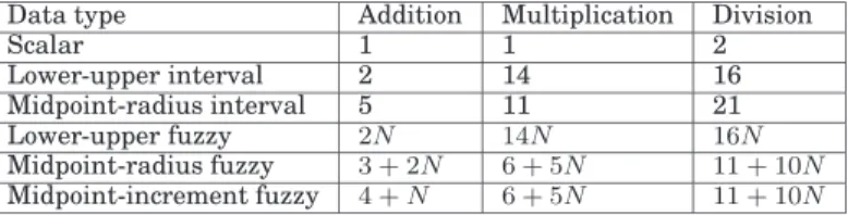
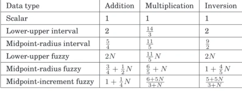
Table III shows the number of instructions, such as basic operations with different rounding, minimum, maximum and absolute value, required in the addition, multiplication and

The minimum and maximum number of rational points on jacobian surfaces over finite fields..

In this section, we will present some further results on the spectrum such as the question of characterizing the image of the spectrum and the subdifferential of a function of

Triangular and trapezoidal membership functions retained in this work are defined using 4 linear functions, completely described by 5 points (a, b, c, d and e) as defined in Equations

(4) Remark 2 We note that, for bounded and continuous functions f, Lemma 1 can also be derived from the classical Crofton formula, well known in integral geometry (see for

We now apply our main result to the computation of orness and andness average values of internal functions and to the computation of idempotency average values of conjunctive