Derivation of a slow phase model of vortex-induced vibrations for smooth and turbulent oncoming flows

YJFLS: 103145 Model 3G pp. 1–32 (col. fig: nil)

Journal of Fluids and Structures xxx (xxxx) xxx

Contents lists available atScienceDirect

Journal of Fluids and Structures

journal homepage:www.elsevier.com/locate/jfs

Derivation of a slow phase model of vortex-induced vibrations

for smooth and turbulent oncoming flows

Vincent

Denoël

Structural & Stochastic Dynamics, University of Liège, Liège, Belgium

a r t i c l e i n f o

Article history:

Received 24 February 2020 Received in revised form 15 July 2020 Accepted 4 September 2020 Available online xxxx Keywords: Wake-Oscillator model Facchinetti model Synchronization

Stochastic Van der Pol oscillator Lock-in

Turbulence

a b s t r a c t

This paper analyzes the influence of turbulence on a wake-oscillator model. Turbulence is introduced by randomizing the model proposed by Facchinetti et al. under the quasi-steady assumption. A multiple scale analysis of the deterministic model shows that the response is governed by a dimensionless groupD, expressed as a function of the amplitudes of the forcing terms in the two governing equations, the total (aerodynamic plus structural) damping and the parameterεof the fluid Van der Pol oscillator. The influence of turbulence is interpreted as a stochastic noise of small intensity and with a slower timescale than the (fast) oscillations, which is typical of wind engineering applications. A slow phase model of the problem is then derived by assuming that the small turbulence drives the system only slightly away from its limit cycle in smooth flow conditions. Standard modeling techniques borrowed from other fields of physics, in particular the observation of phase shifts and their accumulation, are used to highlight conditions under which the turbulence of the oncoming flow might reduce the amplitudes of vibrations of the body. The slow phase model is derived in smooth flow conditions, then extended to turbulent flow. It recalls that the phase plays a central role in synchronization problems, and that the response amplitude should only be considered as a sub-product of the slow phase. The slow phase model is expressed by means of a first order nonlinear differential equation for the phase and a memoryless transformation for the response amplitudes. Its solution is explicit and simple in some limiting cases. In particular, for small turbulence intensity, the response is shown to be insensitive to turbulence when its frequency content is not low enough. This major dependence upon the frequency content of the turbulence explains that the reduction of VIV due to turbulence cannot be explained by the turbulence intensity only, as usually considered today. The required relative smallnesses of the turbulence and its frequency content naturally appear in the derivation, which is led in a dimensionless manner. Finally, the present study constitutes an analysis of a phenomenological model which could be used in a much wider concept than of the elastically-mounted circular cylinder.

© 2020 Elsevier Ltd. All rights reserved.

1. Introduction 1

Models describing vortex-induced vibrations (VIV) of bodies immersed in smooth flows are based on an equation of 2 motion for the structural vibrations which is appropriately modified or complemented in order to model the interaction 3 with the fluid in a more or less sophisticated manner. Existing two-dimensional models are typically classified in three 4 different families (Païdoussis et al.,2010). In family I (forced), the fluid is modeled as a passive external lift force on the 5

E-mail address: v.denoel@uliege.be.

https://doi.org/10.1016/j.jfluidstructs.2020.103145 0889-9746/©2020 Elsevier Ltd. All rights reserved.

Please cite this article as: V. Denoël, Derivation of a slow phase model of vortex-induced vibrations for smooth and turbulent oncoming flows. Journal of structural oscillator; the root-mean-square value of the lift is calibrated with ad hoc measurement (Simiu and Scanlan, 1

1996). In family II (forced feedback), the lift force depends on the state –usually the amplitude– of the structural oscillator. 2

The model consists therefore in a nonlinear differential equation which is capable of modeling the self-limiting features 3

of this problem (e.g. Larsen, 1995; Lupi et al., 2018; Marra et al., 2011). In family III (wake-oscillator), the fluid is 4

more accurately modeled as a dynamical system with a limit cycle. A Van der Pol or Rayleigh differential equation is 5

typically used for this and is coupled with the structural oscillator in various possible ways (Hartlen and Currie,1970; 6

TAMURA and Matsui,1980;Krenk and Nielsen,1999;Facchinetti et al.,2004;Farshidianfar and Zanganeh,2010). After 7

an exhaustive analysis,Facchinetti et al.(2004) suggested to adopt a forcing of the fluid equation which is proportional 8

to the acceleration of the elastic body. Tamura’s model (TAMURA and Matsui,1980) is based on a formal derivation and 9

physical arguments. By combining the velocity and acceleration of the body into the forcing term of the fluid, it is more 10

general than Facchinetti’s model. It is for instance able to mimic the asymmetry of the lock-in response, as in the seminal 11

Birkhoff(1953) orHartlen and Currie(1970) models. 12

The influence of turbulence on VIV of elastically mounted cylinders or more complicated shapes like bridge decks has 13

been experimentally investigated in many studies (Howell and Novak,1980; Matsumoto et al.,2001; So et al.,2008; 14

Trush et al., 2017). It appears that there is no clear consensus on the influence of turbulence. Anyways, the answer 15

shall not necessarily be dichotomic; at least, the influence of turbulence should depend on the type of turbulence (its 16

frequency content) and its intensity. In some studies, turbulence is shown to have a strong effect on the synchronization 17

mechanism and may lead to a complete suppression of VIV (Cao and Cao,2017). Other works tend to indicate that the 18

grid turbulence of the oncoming flow has virtually no influence on the response amplitude (Goswami et al.,1993). The 19

divergent conclusions of these studies indicate the complexity of the problem. In fact, the flow physics in the whole lock-in 20

regime is much more complex than the von Karman vortex street, which appears for fixed bluff bodies (Williamson and

21

Roshko,1988; Pasto,2008). Computational fluid dynamics simulations have shed a different light on the problem and 22

helped understand the peculiarities of the flow, locally, where detachment is affected by turbulence (Guilmineau and

23

Queutey,2004;Nguyen et al.,2018). Yet, the analysis that is carried out in this paper does not pretend to enter such a 24

detailed level of analysis and, quite the opposite, aims at analyzing a simple and adjustable phenomenological model. 25

Available mathematical models to describe VIV in a turbulent oncoming flow are much scarcer than for smooth flows. 26

Civil engineering applications such as bridge aerodynamics (Hansen,2007;Komatsu and Kobayashi,1980;Larsen,1995; 27

Sarwar and Ishihara,2010;Wu and Kareem,2013), cable aerodynamics (Dyrbye and Hansen,1996; Matsumoto et al., 28

2001;Denoël and Andrianne,2017), chimneys (Daly,1986;Pritchard,1984; Ruscheweyh and Sedlacek,1988) and tall 29

buildings (Kawai,1992) are all concerned by vortex induced vibrations in the atmospheric boundary layer where the 30

magnitude of the fluctuating component (turbulence) can reach up to 20% or more of the average wind velocity. There 31

are therefore obvious needs for simple models of VIV in the presence of noise. In the family of externally forced models 32

(family I), Vickery and coworkers (Vickery and Clark,1972;Vickery and Basu,1983;Vickery,1995,1998) have proposed 33

a loading model of tapered stacks which is still widely used today. It constitutes a cornerstone of the modeling of the 34

influence of turbulence on vortex-induced vibrations. This model has been constructed as a simple generalization of the 35

externally forced model (family I), by modeling the aerodynamic loading as a narrow band stochastic process, instead of 36

a deterministic harmonic loading. Stochastic versions of the family II models are also available in the literature, see e.g. 37

Le and Caracoglia(2015). Following the same spirit, this paper presents and analyzes a randomized version of a simple 38

wake oscillator model (family III). A seminal randomized version of the Hartlen–Currie model is studied in Benaroya

39

and Lepore(1983) by means a convolution integral of the linear structural oscillator and the derivation of the Fokker– 40

Planck–Kolmogorv equations for the nonlinear fluid equation, externally forced by a narrow-band stochastic structural 41

motion. Using a Monte Carlo approach, Krenk’s wake-oscillator model, based on an energy balance, has been studied in 42

stochastic conditions using the quasi-steady approach too (Nielsen and Krenk, 1997), after which it is concluded that 43

the stochastic response resembles the observed behavior in experiments and full-scale testing. Monte Carlo simulations 44

are the simplest way to tackle non deterministic problems since the solution just requires the generation of synthetic 45

realizations of the turbulent flow and the statistical analysis of the response (Tagliaferri and Srinil,2017). This approach 46

has also been used to determine the response of structures with many more degrees-of-freedom (Li,2019) or in more 47

complicated geometries than the 2-D case of simple wake-oscillator models (Ulveseter et al.,2017). Although being simple 48

to implement, the Monte Carlo approach does not offer the same depth of understanding as explicit closed form solutions 49

which are only valid in some simple configurations, e.g. in the analysis of the Van der Pol equation alone in stochastic 50

loading conditions (Leung,1995;Gu et al.,2011). More recently Facchinetti’s wake-oscillator model has also been studied 51

in stochastic conditions, under the quasi-steady assumption. While Aswathy and Sarkar study the stochastic version of 52

this model and the influence of parametric noise with the help of Monte Carlo simulations (Aswathy and Sarkar,2019), 53

Shoshani examines the responses of the coupled system by means of stochastic averaging (Shoshani,2018). 54

As explained above the quasi-steady assumption shall not strictly apply, nor be used in a predictive manner (a simple 55

argument is to observe that both the Strouhal number and the aerodynamic coefficients are affected by turbulence of 56

the oncoming flow), it is still interesting to understand the specific features of a model. This paper does not pretend to 57

offer more that the understanding of a phenomenological model, that could be fitted to observed experimental or in-situ 58

measured data. With this in mind, this paper analyzes the stochastic version of the Facchinetti model with the pragmatical 59

tools of nonlinear stochastic dynamics. Quite interestingly, it also introduces a slow phase model for this problem. As 60

seen next, this model is simple enough to derive approximate solutions of the problem, encapsulating the major problem 61

YJFLS: 103145

V. Denoël / Journal of Fluids and Structures xxx (xxxx) xxx 3

parameters in the governing leading dimensionless groups. This approach might be attractive to complement attempts at 1 standardizing the design of VIV-sensitive structures (Hansen,2007;Standard,1991). 2 The paper is organized as follows. In Section 2, the considered (Facchinetti) model is introduced, together with 3 its randomized version. The averaged version of the deterministic system is introduced in Section 3. This derivation 4 emphasizes the central role of the dimensionless groupDand the slow phase between the structural and fluid oscillators. 5 It is also emphasized that it is not necessary to resolve the fast dynamics as long as the slow dynamics of the phase and 6 the response envelopes are studied. In Section4, the stochastic version of the problem, is presented. Phase slips and their 7 accumulation are evoked to explain why and how turbulence is able to affect the VIV response. Then, a slow phase model 8 is derived and simple analytical solutions are provided. They offer a simple outlook on the parameters and dimensionless 9 groups driving the response of the coupled system in stochastic conditions. Illustrations are finally given to feed the 10

discussion about the validity of the proposed simplified solutions. 11

Nomenclature 12

Model parameters Units Scaling Dimensionless

t T, T−1 _{Time t}⋆

₌

₁

_/ω

0

τ

y(t) L Transverse displacement of cylinder y⋆

=

ε

D Y

(τ,

T

=

ετ)

q(t) – Generalized lift (Fdlb model) q⋆

=

1 Q

(τ,

T

=

ετ)

ε

– a _{van der Pol coefficient in wake equation}

D L Crossflow dimension of cylinder

ω

0 T−1 Natural circular frequency of elastically

mounted cylinder

mS, mF, cS, kS, mixed Parameters of the Facchinetti–de

Langre–Biolley...

ρ

, U∞, CD, CL0,A0 mixed ...model (Fdlb), see definition in(1)

µ

– Fluid/Structure mass ratio

(

µ =

_4(mρπD2 S+mF)

=

ρ ρS), see(4) M0 St – Strouhal number

fshedding T−1 Shedding frequency (fshedding

=

StU∞

/

D)

Sc⋆

=

Sc

ξ/ξ

s – Scruton number, defined with total damping, see(17)

SG⋆

=

SG

ξ/ξ

s – Skop–Griffin number, defined with total damping, see(18)

u(

τ

) L T−1 Turbulence velocity (Gaussian random process)

σ

u U

(

T

=

ετ)

σ

u L T−1 Standard deviation of turbulence velocity Iu – a Turbulence intensity (Iu

=

σ

u

/

U∞)

Su L2T

−1 _{Power spectral density of turbulence}

_σ

2

u

/ω

0 SU

( ˜ω = ω/ω

0

)

α

– a _{Dimensionless characteristic turbulence}

frequency

13

Model parameters Units

M0 – Dimensionless fluid/structure mass ratio, see(10)

ξ

s,

ξ

a – a Structure and fluid damping ratios, see(4)

ξ = ξ

s

+

ξ

a – a Total damping ratio, see(4)

Ω – b _{Mistuning, bifurcation parameter, see(4)}

δ = (

Ω

−

1

) /ξ

– Centered and scaled mistuning, bifurcation parameter, see(22)

D – Unique dimensionless group characterizing the deterministic response of the Fdlb model, see(28)

Ry

(

T

)

– Slow envelope of the structural responseY Rq

(

T

)

– Slow envelope of the reduced liftQ

ψ

(T ) – Slow phase betweenY(

τ,

T ) andQ(

τ,

T )

ξ

0

=

ξ/ε

– Reduced damping ratio

I0

=

Iu

/ε

– Reduced turbulence intensity Υ(T )

=

cot

ψ

(T ) – Cotangent of the slow phase, see(45)

ΥLC

=

cot

ψ

LC – Cotangent of the slow phase on the limit cycle,ΥLC

≡

ΥLC

(δ;

D

)

, see(27)

B – Dimensionless group characterizing the stochastic response of the Fdlb model, see(47)

V – VIV reduction factor accounting for the frequency content of turbulence (vs. the slow memory of the structure), see(54)

Please cite this article as: V. Denoël, Derivation of a slow phase model of vortex-induced vibrations for smooth and turbulent oncoming flows. Journal of Model parameters Units

∆Υ(T ) – Deviation from limit cycle solution∆Υ(T )

=

Υ(T )

−

Υ_LC

µ

∆Υ,

σ

∆Υ – Average and standard deviation of the deviation from limit cycle solution

µ

Υ,

σ

Υ – Average and standard deviation of the cotangent of the slow phase,

µ

Υ

=

µ

_∆Υ

+

Υ_LC,

σ

_Υ

=

σ

_∆Υ

ry – Reduction factor of the maximum structural response, random variable 1

Symbols with a naught underscore

·

₀indicate quantities that have been scaled by a power of

ε

(

ξ

0,I0,A0,M0). Calligraphic

symbols are used to represent dimensionless numbers or groups. 2

a_{Small numbers.}

3

b_{Bifurcation parameter centered around unity (lock-in range).}

4

2. Considered wake-oscillator model

5

The Facchinetti–de Langre–Biolley (Fdlb) model reads (Facchinetti et al.,2004) 6

(

mS

+

mF

) ¨

y

+

(

cS

+

CD 2

ρ

U∞D

)

˙

y

+

kSy

=

1 4

ρ

U 2 ∞DCL0q (1) 7

¨

q

+

2

π

StU∞ D

ε (

q 2

₋

₁

_{) ˙}

_q

₊

(

2

π

StU∞ D

)

2 q

=

2A0

¨

y D (2) 8

where y(t) (units:L) and q(t) (units: -) represent the two degrees-of-freedom associated with the cross-flow structural 9

motion and the lift force resulting from vortex shedding. The parameters of the model are mS, cSand kS, the mass, viscosity

10

and stiffness of the structure (per unit length), D the cylinder diameter (or characteristic cross-flow dimension),

ρ

and U∞

11

the density and the constant velocity of the fluid, CDand CL0the stationary drag and the magnitude of the lift fluctuations 12

on the fixed body and St the Strouhal number. FinallyA0 is a dimensionless parameter related to the influence of the

13

structural motion on the dynamics of the wake (2A₀corresponds to symbol A used inFacchinetti et al.,2004), while

ε

is 14

another dimensionless parameter that describes the memory in the wake equation and is related to the magnitude of the 15

nonlinearity in the Van der Pol equation for the wake, therefore to the strength of the limit cycle. The equivalent mass of 16

displaced fluid mF

=

CM

ρ

D2π₄ (which is negligible in wind engineering applications) is added to the structural mass mS

17

in order to define the structural circular frequency

ω

0

=

√

kS

/(

mS

+

mF

) =

√

kS

/

m. The Fdlb model has been imagined

18

for subcritical flows 300≲Re≲1

.

5

·

105(Facchinetti et al.,2004). Addition of turbulence in the oncoming flow is known 19

to promote early transition to supercritical (Blackburn and Melbourne,1996), which truncates the domain of applicability 20

of this model. 21

2.1. Dimensionless version of problem 22

A dimensionless version of the governing equations is obtained by introducing the characteristic time t⋆

=

1

/ω

0and

23

a characteristic structural displacement y⋆(to be defined soon) and defining 24

τ =

t t⋆

,

Y(

τ

)

=

y [t(

τ

)] y⋆ and Q(

τ

)

=

q [t(

τ

)] q⋆ (3) 25

with q⋆arbitrarily chosen as 1. With the usual dimensionless numbers, characterizing the structural damping ratio

ξ

sand 26

aerodynamic damping ratio

ξ

a, as well as the reduced wind velocityΩ and the mass ratio

µ

27

ξ

s

=

cS 2

√

kSm

, ξ

a

=

ρ

U∞D 4

√

kSm CD

,

Ω

=

StU∞

/

D

ω

0

/

2

π

=

fshedding f0

, µ =

ρπ

D2 4m

=

ρ

ρ

S

,

(4) 28

with

ρ

Sthe equivalent density of the cylinder, the governing equations become

Y′′

+

2

(ξ

s

+

ξ

a

)

Y ′

+

Y

=

1 4 1 kSy⋆

ρ

U∞2DC 0 LQ

=

µ

4

π

3 D y⋆

(

Ω St

)

2 C_L0Q (5) Q′′

+

ε

Ω

(

Q2

−

1

)

Q′

+

Ω2Q

=

2A₀y ⋆ DY ′′ (6) where the prime symbol denotes derivatives with respect to the dimensionless time

τ

. In the wake equation, the small 29

parameter

ε

plays a major role. It is small to moderate, say in the range

[

0

.

01

;

0

.

4

]

; it is always certainly not equal to 30

zero, otherwise there would not be any synchronization. It appears therefore as a good candidate to derive an asymptotic 31

solution of this problem. In order to derive a consistent distinguished limit, we study the solutions of the problem where 32

the structural displacement y is small compared to the diameter D of the body, which anyways correspond to the domain 33

of applicability of the wake-oscillator model (2-S shedding mode, see e.g.Williamson and Roshko,1988). It is therefore 34

natural to choose 35

y⋆

=

ε

D (7)

YJFLS: 103145

V. Denoël / Journal of Fluids and Structures xxx (xxxx) xxx 5

as a characteristic displacement, and to solve the problem forY(

τ

)

∼

1. Seeking applications in wind engineering, the (fluid-over-structure) mass ratio is assumed to be very small, of the order of

ε

2_{or smaller (typically 10}−3_{). The mass ratio}

µ

is therefore written

µ = µ

0

ε

2with

µ

0

∼

1 so that the governing equations become

Y′′

+

2

(ξ

s

+

ξ

a

)

Y

′

+

Y

=

2

ε

M₀Ω2Q (8)

Q′′

+

ε

Ω

(

Q2

−

1

)

Q′

+

Ω2Q

=

2

ε

A₀Y′′ (9)

whereM0

∼

1 has been defined as 1

M₀

:=

µ

8

π

3

_ε

2

C_L0

St2

.

(10) 2

It therefore carries information about the mass ratio, the lift force and the shape of the body (through the Strouhal number 3 and lift coefficient). The Skop–Griffin parameter is expressed as a function ofM0because it is the sole dimensionless group 4

carrying information about the mass ratio. The smallness of the righthand side of(8)also translates that the lift created 5 by vortex shedding is small compared to the elastic forces in the body (energy is slowly pumped in/out of the system). 6 In this paper, the turbulence of the oncoming flow is introduced in the model, following the quasi-steady ap- 7 proach (Simiu and Scanlan,1996;Dyrbye and Hansen,1996). A randomized version of the governing equations, obtained 8 by substituting U∞

+

u(t) for U∞in(8)–(9)is here developed. It is assumed that u(t) is a zero-mean Gaussian stochastic 9

process with known variance

σ

uand known power spectral density Su(PSD). The validity is this randomization procedure 10 is still debatable with regards to the available information today, although this is common practice as stated in the 11 introduction; however, seeking applications in the atmospheric boundary layer, the turbulence of the oncoming flow 12 is characterized by a slow timescale which is one or several orders of magnitude slower than the structural oscillations 13 and, hence, aeroelastic effects. This argument contributes to the separation of the aeroelastic and buffeting effects, which 14 is favorable to this decomposition, (seeCremona et al.,2002, p.88). Noticing that U∞appears in the definition of

ξ

aand 15 Ω, this substitution readily provides the resulting system of equations in its most simple form, 16

Y′′

+

2

(ξ

s

+

ξ

a

(

1

+

IuU

))

Y ′

+

Y

=

2

ε

M0

(

1

+

IuU

)

2Ω2Q Q′′

+

ε

Ω

(

1

+

IuU

) (

Q2

−

1

)

Q′

+

Ω2

(

1

+

IuU

)

2Q

=

2

ε

A0Y ′′ (11) 17

where a dimensionless turbulence U(

τ

) has been defined by normalizing the velocity fluctuation u(t) by is standard 18

deviation

σ

u, 19

u [t

(τ)

]

=

σ

_uU(

τ

)

=

IuU∞U(

τ

)

,

(12) 20

with Iu

=

σ

u

/

U∞the turbulence intensity, usually in the range

[

0

;

0

.

25

]

; it is therefore considered as a small number, 21

i.e. Iu

≪

1. 22

The objective of the study reported in this paper is to analyze this set of equations with the qualitative and quantitative 23 tools in nonlinear dynamics, in order to sketch the important features of this model and explain them with simple 24 concepts. As seen next, this will provide a possible explanation of the influence of turbulence on the lock-in phenomenon. 25 In Sections3and4we derive an asymptotic solution of this problem. In Section5, we study the accuracy of the proposed 26 model by comparison with Monte Carlo simulations of(11), which will serve as a reference solution. 27

2.2. The dimensionless turbulenceU(

τ

) 28

In the governing equations,U(

τ

) is a zero-mean unit-variance process indexed on the dimensionless time

τ

(

µ

U

=

0, 29

σ

U

=

1). The corresponding PSD can be expressed as a function of the power spectral density of u(t), sinceU(

τ

) and u(t) 30

are related to each other by means of a stretch and a re-scaling. Let us write Su

(ω;

p

)

the PSD of u(t), where p represents 31 some possible parameters of the model such as

σ

u, the variance of u(t), or the turbulence lengthscale Lxu, or the mean 32

wind velocity U∞. For instance, the following PSD’s 33

Su

(

ω;

U L

, σ

2 u

)

=

σ

_u2 0

.

546 L U

(

1

+

1

.

64L U

|

ω|)

5/3

,

Su

(

ω;

a

, σ

_u2

) =

_σ

2 u a

π

1

ω

2

₊

_a2

,

(13) 34

represent an existing model of the power spectral density of atmospheric turbulence (Dyrbye and Hansen,1996) and the 35 power spectral density of the Ornstein–Uhlenbeck process (Papoulis and Pillai,2002). This latter example will be used in 36 the following illustrations. The PSD of the zero-mean unit-variance processU(

τ

) is then given by 37

SU

( ˜ω; α) =

ω

0

σ

2 u Su

( ˜

ω ω

0

;

α ω

0

, σ

u2

)

(14) 38 where

ω = ω/ω

˜

₀is the dimensionless frequency parameter (associated with time

τ

) and

α

a dimensionless characteristic 39 frequency of the turbulence velocity. For the two examples given above

α =

U

/

L

ω

0and

α =

a

/ω

0, respectively. This 40

number relates the characteristic frequency of turbulence (U

/

L or a) to the characteristic frequency

ω

0of the structure. 41

Please cite this article as: V. Denoël, Derivation of a slow phase model of vortex-induced vibrations for smooth and turbulent oncoming flows. Journal of

Table 1

Typical range of variation of the parameters of the problem.

Model Range of Governing Range of Reduced Range of

parameters variation parameters variation parameters variation

ξs [5·10−4,10−2] Ω [0.5,1.5] D [1;30] ξa [10−3,5·10−2] ε [0.05;0.3] ξ0=ξ/ε [5·10−2;1] ξ = ξs+ξa [10−3,5·10−2] I0=Iu/ε [0;10] Turbulence M0 [0.01;1] α [10−3_;10−1_{] A} 0 [1;10] Iu [0;0.25]

sequel in order to derive closed-form solutions of this problem. The PSDs of the normalized turbulence corresponding to 1

(13)are therefore given by 2 SU

( ˜ω; α) =

0

.

546

(

α

3/5

₊

₁

.

₆₄

_{| ˜}

ω|)

5/3

,

SU

( ˜ω; α) =

α

π

1

˜

ω

2

₊

α

2

.

(15) 3

The normalization property of the PSD translates into 4

∫

+∞

−∞

SU

( ˜ω; α)

d

ω =

˜

1 (16)

5

regardless of the value of the parameter

α

(Denoël and Carassale,2015). Notice that SU

( ˜ω; α)

might be expressed as a

6

function of additional parameters, should the original density Su

(ω)

be more complex than(13). It is just independent of 7

σ

uas a result of the re-scaling. 8

2.3. Order of magnitude of the parameters of the model 9

In typical applications,

ξ

s,

ξ

a,

ε

,

α

and Iuare small parameters. The orders of magnitude of the parameters of the model 10

are given inTable 1while the numerical values that are chosen in the following illustrations (Data Set 1 and Data Set 11

2) are given inTable 2. These values are inspired from the examples given inTAMURA and Matsui(1980) (Data set 1) 12

andFacchinetti et al. (2004) (Data set 2). Some other important rescaled parameters such as

ξ

0

=

ξ/ε = (ξ

s

+

ξ

a

) /ε

13

and dimensionless groups such asD

=

A0M0

/ξ

02 will naturally appear in the following developments. In order to be

14

exhaustive and collect all relevant information at the same place, the values for these dimensionless groups are also 15

reported in the same Tables. The origin of these parameters will become clearer in Sections3and4. 16

The parameters of the Fdlb model can be related to other standard mass-damping parameters that are used to describe 17

vortex-induced vibrations. In particular, using the standard definition for the Scruton number (Scruton,1981) 18 Sc⋆

:=

4

π (ξ

s

+

ξ

a

)

m

ρ

D2

=

π

2

ξ

µ

,

(17) 19

but referring to the total damping

ξ

(instead of only the structural damping

ξ

s), with

µ

the mass ratio defined in(10)and 20

ξ = ξ

s

+

ξ

athe total damping, the Skop–Griffin parameter defined by SG⋆

:=

2

π

St2Sc⋆(Griffin and Koopmann,1977) is 21 found to be given by 22 SG⋆

=

2

π

3St2

ξ

µ

=

ξ

C0 L 4

ε

2_M 0

.

(18) 23

These notations are different from the usual mass-damping parameter SG which is calculated with the structural damping 24

only, SG

=

2

π

3St2

ξ

s

/µ

, or from the usual Scruton number Sc

=

π

2

ξ

s

/µ

also defined for the structural damping only. 25

Rewriting the former equation, it is seen for instance that 26 4M0

ξ

ε

2

=

4M0

ξ

0

ε =

CL0 SG⋆ and D

=

A0M0

ξ

2 0

=

A0

ε ξ

0 C0 L 4SG⋆

.

(19) 27

These relations allow to translate the main results of the following analysis, which are presented with the parameters of 28

the wake-oscillator model, into more usual dimensionless numbers. 29

The smallness of the five parameters

ξ

s,

ξ

a,

ε

,

α

and Iuis fully exploited in the following developments by means of a 30

perturbation approach. This makes possible the establishment of analytical expressions for the stochastic response of the 31

wake-oscillator model. 32

YJFLS: 103145

V. Denoël / Journal of Fluids and Structures xxx (xxxx) xxx 7

Table 2

Considered numerical values used for the illustrations. Below first separation: derived quantities.

Data Set 1 Data Set 2

Model Dimensionless Dimensionless

parameters parameters parameters

ε ε =0.05 ε =0.2 ξs ξs=0.015 ξs=0.0075 ξa ξa=0.015 ξa=0.0075 M0 M0=0.9 M0=0.0187 A0 A0=1 A0=6 α Variable Variable Iu,I0=Iu/ε Variable Variable ξ = ξs+ξa ξ =0.03 ξ =0.015 ξ0=ξ/ε ξ0=0.6 ξ0=0.075 D D=2.5 D=20 ξ (1+D) ∆Ω = ±0.105 ∆Ω = ±0.315

3. Deterministic wake-oscillator model 1

3.1. Averaged governing equations 2

When the turbulence is discarded (U

(τ) =

0 or Iu

=

0), the set of equations boils down to the governing equations 3

studied byFacchinetti et al.(2004), 4

Y′′

+

2

ξ

Y′

+

Y

=

2

ε

M0Ω2Q

Q′′

+

ε

Ω

(

Q2

−

1

)

Q′

+

Ω2Q

=

2

ε

A₀Y′′ (20) 5

where

ξ = ξ

s

+

ξ

arepresents the sum of structural and aerodynamic dampings. We only focus on the specific case where 6

{

ξ, ε} ≪

1 and this is formalized by introducing 7

ξ = ξ

s

+

ξ

a

=

ξ

0

ε

(21) 8

where

ξ

0

∼

1 (is of order 1 at most). We also focus on small mistuning conditions, i.e. assume that the vortex shedding 9

frequency of the fixed cylinder is close to the natural frequency of the structure. This is formalized by writing 10

Ω

=

1

+

ξ δ =

1

+

ξ

0

ε δ ⇔ δ =

Ω

−

1

ξ

=

fshedding

−

f0

ξ

f0 (22) 11 where

δ ∼

1 is a detuning parameter of order 1. The detuning is scaled with respect to

ξ

which might appear unusual at 12 first glance. In the forced case where the same problem is reconsidered by imposing a prescribed motion to the body, the 13 structural damping ratio vanishes and the proper scaling is

ω = (

Ω

−

1

) /ε

, seeAppendix A.2. The choice to scale here 14 the mistuning with

ξ

, in the free vibration test, will appear natural in the light of the following results. 15

The set of governing Eqs.(20)is then solved by considering a multiple scales solution, in the form of the following ansatz

Y(

τ; ε

)

=

Y0[

τ,

T

(τ) ; ε

]

+

ε

Y1[

τ,

T

(τ) ; ε

]

+ · · ·

Q(

τ; ε

)

=

Q₀[

τ,

T

(τ) ; ε

]

+

ε

Q₁[

τ,

T

(τ) ; ε

]

+ · · ·

(23)

whereY_iandQ_i(i

=

0

,

1

, . . .

) are of order 1, which indicates that the solution is sought as a function of a fast time

τ

and 16 a slow time T chosen as T

=

ετ

. Application of standard techniques in multiple timescales (Bender and Orszag,2013) 17

shows that the leading order solution of the set of governing equations is 18

Y₀

=

Ry(T ) cos [

τ + ϕ

(T )]

;

Q0

=

Rq(T ) cos [

τ + ϕ

(T )

+

ψ

(T )] (24) 19 where the slowly varying amplitudes Ry(T ), Rq(T ) and the relative phase

ψ

(T ) satisfy the secularity equations (see details inAppendix A.1) R′_q

=

A0Rysin

ψ −

1 8R 3 q

+

1 2Rq R′_y

=

M₀Rqsin

ψ − ξ

0Ry

ψ

′

=

(

A0 Ry Rq

+

M0 Rq Ry

)

cos

ψ + ξ

0

δ.

(25)

This way of averaging the governing equations reveals that the 4-dimensional dynamical system described by the 20 original Eqs. (11)in the state-space actually evolves on a 3-dimensional subspace, at leading order. This is consistent 21

Please cite this article as: V. Denoël, Derivation of a slow phase model of vortex-induced vibrations for smooth and turbulent oncoming flows. Journal of with the usual features of multiple scale analysis in the time (Bender and Orszag, 2013) or frequency (Denoël, 2015) 1

domains. 2

The multiple scale analysis that has resulted in the averaged Eqs.(25)has some advantages compared to assuming 3

delayed harmonic responses forYandQas inFacchinetti et al.(2004): (i) it explicitly introduces the slow amplitude and 4

slow phase, (ii) it also explicitly introduces the governing equation for the dynamics of the slow phase, the third equation 5

in(25), which is a central concept in synchronization, (iii) final results take simple expressions since they correspond to 6

secularity conditions instead of long derivations involving trigonometry and algebra. On the flip side, the mistuning needs 7

to be small. 8

3.2. The slow phase on the limit cycle 9

The steady state solution is obtained when the time derivatives on the lefthand sides in(25)vanish. In particular the 10

second equation yieldsM₀Rqsin

ψ = ξ

0Ry, so that the ratio 11 Ry Rq

=

M0

ξ

0 sin

ψ

(26) 12

is known and its substitution into the last equation indicates that the phase on the limit cycle cot

ψ

LCthus satisfies

13 cot3

ψ

LC

+

δ

cot2

ψ

LC

+

(

1

+

A0M0

ξ

2 0

)

cot

ψ

LC

+

δ =

0

.

(27) 14

If the lefthand side

ψ

′

had been kept, this would have provided the slow phase model in smooth oncoming flow conditions. 15

It is not written here since only the limit cycle usually matters in smooth flow conditions. The phase on the limit cycle 16

ψ

LC

≡

ψ

LC

(δ,

D

)

only depends on the mistuning

δ

and on the dimensionless group

17 D

:=

A0M0

ξ

2 0

=

A0M0

ξ

2

ε

2

₌

2A0

ε

1 2

ξ

ρ

U2 ∞CL0 8kS

=

A0

ε ξ

0 C0 L 4SG⋆

.

(28) 18

This group translates the relative magnitude between the two (small) forcing terms in the coupled governing equations. 19

Since the mistuning parameter

δ

appears in all even powers of cot

ψ

LCand only there, at leading order, the phase on

20

the limit cycle

ψ

LCis symmetric with respect to

δ

, i.e. not affected by a change of sign of

δ

. As a consequence, the lock-in

21

domain is symmetric with respect to the reduced velocity. This is an important feature of the Fdlb model. 22

General solution. If

δ =

0, the polynomial(27)in cot

ψ

LC has only one real root (becauseD

>

0) corresponding

23

to cot

ψ

LC

=

0, i.e.

ψ

LC

= ±

π₂, which corresponds to a perfect lock-in condition. Indeed, as seen next, this maximizes

24

the response of the system (it is possible to anticipate that a phase shift of

±

π

2 maximizes the energy pumped into the

25

structural degree-of-freedom). Invoking Descartes’ rule of sign, it is observed that the polynomial(27)has one or three 26

positive roots if

δ <

0 and one or three negative roots if

δ >

0. Furthermore, using Cardano’s formula, it is possible to 27

prove that, ifD

<

8, there is only one real root no matter the value of

δ

. On the contrary, ifD

>

8, there are three roots 28

if

|

δ|

lies in the interval

[

I(−)

;

I(+)

]

and only one root otherwise. The bounds of this interval are given by 29 I(±)

=

√

D2

₊

_20D

₋

₈

_±

√

_D

(

_D

₋

₈

)

3 2

√

2

.

(29) 30

The upper bound can be approximated by I(+)

≃

(

4

+

D

)

√

3

4 for values ofDin the range

[

8

, ∼

20

]

, which corresponds to

31

typical applications. 32

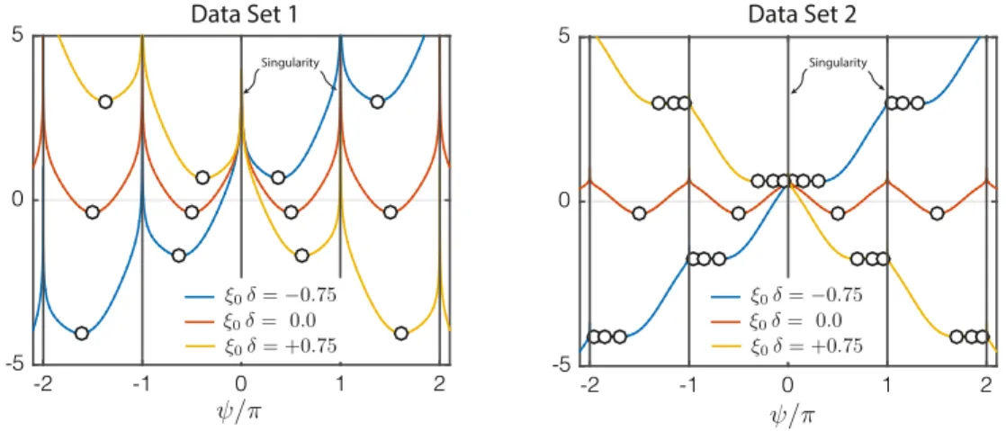
The existence of three real roots is associated with some hysteresis in the model (Païdoussis et al., 2010).Fig. 1

33

represents the one or three roots of the polynomial equation as a function of

δ

and for various values ofD. The figure 34

indeed illustrates that there is only one root forD

<

8 and therefore no hysteresis (blue lines), while there might be 35

three real roots and hysteresis in the system forD

≥

8 (red lines). 36

Exact solutions of the 3rd degree polynomial(27) can be obtained by means of Cardano’s formula. The resulting 37

expressions are rather long; they are not reported here. Instead we focus on simple approximate solutions. 38

Small-root asymptote (Bulk of lock-in region). Let us examine first the conditions under which it is possible to have 39

a small root. This case is the most important since it corresponds to the lock-in phenomenon,

|

cot

ψ

LC

| ≪

1 meaning

40

ψ ≃ ±

π

2. A small-root asymptote is obtained by dropping terms in cot 2

_ψ

LCand cot3

ψ

LCin(27). This yields

41

cot

ψ

small

≃

−

δ

1

+

D

.

(30)

42

This approximation ceases to be valid when either cot3

_ψ

LCeither

δ

cot2

ψ

LCenters in the balance in(27), that is when

43

either (i) cot3

ψ

LC

∼

δ

, i.e.

(

δ

1+D

)

3

∼

δ

or

|

δ| ∼ (

1

+

D

)

3/2, either (ii)

δ

cot2

ψ

LC

∼

δ

, i.e.

|

δ| ∼

1

+

D. All in all, the

44

small-root asymptote is therefore valid when

|

δ| ≪

1

+

D. The small-root asymptote is represented by dashed lines in 45

Fig. 1; this root is represented in the range of validity,

|

δ|

≲1

+

D. 46

YJFLS: 103145

V. Denoël / Journal of Fluids and Structures xxx (xxxx) xxx 9

Fig. 1. Steady-state phase between wake and oscillator on the limit cycle. There are three possible solutions forD≥8 (in red) and just one solution forD<8 (in blue). Represented forD=0,2,4,6 (in blue),D=8 (in black),D=10,12,14,16 (in red). Dashed line represent the small-root and large-root asymptotes. (For interpretation of the references to color in this figure legend, the reader is referred to the web version of this article.)

Large-root asymptote. For

|

δ| >

I(+)_{, far from the center of the lock-in region, there is only one large root, and 1}

the root can be approximated by the solution of cot3

_{ψ + δ}

_cot2

_{ψ =}

_{0, i.e. cot}

_{ψ + δ =}

_{0. Reconsidering the 2}

polynomial(27)we observe that, in the limit case, the independent term balances the term cot

ψ

so that we are left 3 with cot3

_ψ

LC

+

δ

cot2

ψ

LC

+

Dcot

ψ

LC

=

0 whose solution is 4

cot

ψ

large

≃

−

δ ±

√

δ

2

₋

_4D

2

.

(31) 5

This is the asymptotic solution far from the bulk of the lock-in region. It is just given here for information; it is not used 6 in the sequel since it corresponds to a regime that falls out of the lock-in range and is therefore less interesting. This 7

approximate solution is also represented by dashed lines inFig. 1. 8

The extent of the lock-in region. The range of validity of the small-root corresponds to the domain where the fluid 9 and structure oscillators find a steady state solution with a phase shift close to

π/

2, indicating that there is a significant 10 energy exchange between the two oscillators, the fluid one being able to store energy and resulting therefore in large 11 structural oscillations. This translates the so-called lock-in phenomenon observed in vortex-induced vibrations. The size 12 of the lock-in region corresponds therefore to the region where the small-root asymptote is accurate, i.e.

|

δ| ≪

1

+

D. 13 With dimensional parameters, it translates into∆Ω

≪

ξ (

1

+

D

)

. This solution is however only valid under the condition 14 D

<

8, where cot

ψ

LCgrows monotonically with

−

δ

. Indeed, in the caseD

>

8, the folding in the solution is such that the 15

branch associated with the large root can connect the small-root asymptote before it becomes large. In that case, the extent 16 of the lock-in region is precisely given by the upper bound of the interval

[

I(−)

;

I(+)

]

, i.e. approximately

δ < (

4

+

D

)

√

3 4 . 17

Aggregating these two conditions (and using

√

3

3 in the first condition to make the transition fromD

<

8 toD

>

8 18

continuous), the extent of the lock-in regime can be simply expressed by 19

∆Ω

=

ξ

∆

δ =

{

2

ξ (

1

+

D

)

√ 3 3 ifD

≤

8 2

ξ (

4

+

D

)

√ 3 4 ifD

≥

8

.

(32) 20 This proves, as introduced earlier, that the extent of the lock-in region scales with the total damping ratio

ξ = ξ

s

+

ξ

a 21 and that the parameterD, related to the relative amplitude of the coupling terms, finely quantifies this extent. BecauseD 22 is expressed as the product ofA0andM0, it is sufficient that one of the two righthand sides in the governing equations 23

vanishes to obtainD

=

0, i.e. the largest gradient in cot

ψ

LCvs.

δ

, seeFig. 1, and therefore the smallest lock-in domain. 24

The actual influence of the damping ratio on the size of the lock-in domain is actually misleading in this dimensionless 25 formulation. Substituting in(32)the definition ofD, i.e.

ξ

D

=

A0

ε

2M0

/ξ

, this is also equivalent to 26

∆Ω

=

ξ

∆

δ =

⎧

⎨

⎩

2 √ 3 3

(ξ +

A0ε2M0 ξ

)

ifD

≤

8 2 √ 3 4

(

4

ξ +

A0ε2M0 ξ

)

ifD

≥

8 27

Please cite this article as: V. Denoël, Derivation of a slow phase model of vortex-induced vibrations for smooth and turbulent oncoming flows. Journal of In the most usual cases whereD

≫

1 (or evenD

>

8), the second term in the brackets leads even for moderate to large 1

damping ratios, and the extent of the lock-in regime∆Ω tends to decrease with increasing damping. This is consistent 2

with experimental evidences, see e.g.Marra et al.(2015) in air andSoti et al.(2018) in water. 3

Also, as the total structural damping decreases, the width of the peak in the frequency response function of the 4

structural oscillator decreases and the bandwidth over which it is able to interact with the fluid oscillator decreases. 5

This explains why, as

ξ

tends to zero, the size of the lock-in domain is reduced. This might have looked paradoxical; it is 6

important to notice however that the amplitude of the resulting motion increases as

ξ →

0. 7

3.3. The response amplitudes on the limit cycle 8

The phase shift

ψ

plays a significant role in the analysis of the limit cycle and consequently of the possible 9

synchronization in the presence of external forcing. This naturally appears since the first equation to solve is in cot

ψ

, 10

while the determination of Rq and Ry can be seen as a secondary result. Once the phase shift between the fluid and 11

structure oscillators is known on the limit cycle, the amplitude of vibration is obtained by combining the first and second 12

equations in(25). They give 13 A0Rysin

ψ =

1 8R 3 q

−

1 2Rq

=

A0M0

ξ

0 Rqsin2

ψ

(33) 14

from which it is readily seen that Rqand Rysatisfy 15 Rq

=

2

√

1

+

2

ξ

0Dsin2

ψ ;

Ry

=

2 M₀

ξ

0

|

sin

ψ|

√

1

+

2

ξ

0Dsin2

ψ.

(34) 16

In these expressions, the maximum responses Rqand Ryare obtained in perfect lock-in conditions (sin

ψ =

1). NB: we 17

have omitted the subscriptLCin

ψ

, Rqand Ryin order to lighten the notation. The minimum response of the fluid oscillator 18

is 2, consistently with well-established theories about the van der Pol oscillator (Nayfeh and Mook,2008). The magnitude 19

of the structural response on the limit cycle Ryscales with 1

/ξ

0andM0. It is also maximum when sin

ψ

√

1

+

2

ξ

0Dsin2

ψ

20

is maximum, i.e.

ψ = ±π/

2. The mistuning

δ

affects the magnitude of the response through the value of the phase shift 21

ψ

on the limit cycle. These expressions show that the maximum responses on the limit cycle, Rqand Ry

/

M0, only depend

22

on

ξ

0

=

ξ/ε

,Dand

δ

(through

ψ

).Fig. 2shows the amplitude of the response for three values of

ξ/ε

(0.75, 0.50 and

23

0.25), for various values ofD

∈ [

4

;

16

]

, and as a function of parameter

δ

. The black lines correspond toD

=

8, the largest 24

value ofDfor which there is only one solution. ForD

>

8 (red lines), the existence of several roots translates into a 25

‘‘mushroom’’ shape, as opposed to a ‘‘bell’’ shape forD

<

8. The vertical dashed lines in the plots of Ry

/

M0represent

26

the extent of the lock-in domain, as defined by(32). The good agreement with the mushroom or bell shapes indicates 27

that this proposition qualitatively does a good job for all possible values of

ξ

0andD. We also notice that an approximate

28

solution in the bulk on the lock-in region can be obtained by replacing

ψ

in(34)by the small-root asymptote(30). This 29

yields the curved dashed lines represented on the top of the response. 30

Together with the simple expression of the extent of the lock-in domain, this simple expression for the magnitude of 31

the response provides a fair estimate of the amplitude of the response that could be useful for engineering applications. 32

The case of perfect lock-in, when

δ =

0,

ψ =

π₂, is of paramount importance since it corresponds to the maximum 33

structural response, Ry

=

2M_ξ00

√

1

+

2

ξ

0D. With the original parameters of the problem, we obtain

34 ymax D

=

ε

Ry

=

2 M0

ξ

0

ε

√

1

+

2

ξ

0D

=

C0 L 2SG⋆

√

1

+

A0

ε

C0 L 2SG⋆

.

(35) 35

This result is similar to the expression obtained byFacchinetti et al.(2004) with a (single timescale) delayed harmonic 36

ansatz. What the current multiple scale analysis has provided in addition is a complete analysis of the phase on the limit 37

cycle and the extent of the lock-in region. Also, we emphasize that the simple expression given here is expressed as a 38

function of the SG⋆parameter defined with

ξ = ξ

s

+

ξ

a. We chose to do it so because it is the actual quantity that governs 39

the amplitude of the response. The maximum amplitude is unbounded as SG⋆

→

0 because both the structural and the 40

aerodynamic dampings vanish. If only the structural damping vanishes, SG

→

0, the aerodynamic damping remains and 41

the Griffin plot features a saturation at low structural damping. The maximum amplitude is thus obtained by replacing SG⋆ 42

by 2

π

3_St2

_ξ

a

/µ

in(35). The other asymptotic case, SG⋆

→ +∞

shows that ymax

/

D scales as

(

SG⋆

)

−3/2, which is consistent 43

with experimental data, see e.g.Skop and Balasubramanian(1997), where the slope -3/2 is visible in the log–log plot. 44

Eqs.(32)and(35)prove very useful in identifying the parameters of the Fdlb model from experimental data. Once

ξ

45

is known, the measured extent of the lock-in domain yieldsDthrough(32); then(35)consists in an additional equation 46

to determine

ε

andM0once ymax

/

D is known.

47

3.4. Period of the limit cycle 48

The period of the limit cycle is obtained by returning to the leading order solution given in (24), i.e. Y0

=

49

Ry(T ) cos [

τ + ϕ

(T )] andQ0

=

Rq(T ) cos [

τ + ϕ

(T )

+

ψ

(T )]. On the limit cycle, Rq, Ryand

ψ

have converged to steady state 50

YJFLS: 103145

V. Denoël / Journal of Fluids and Structures xxx (xxxx) xxx 11

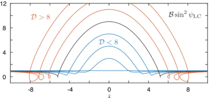
Fig. 2. Maximum responses Rqand Ry/M0on the limit cycle, represented for three values ofξ0=ξ/εand forD=4,6 (in blue),D=8 (in black),

D=10,12,14,16 (in red). Dashed line represent the extent and height of the lock-in region, given by(32)and(34)where cotψ = −δ/(1+D). (For interpretation of the references to color in this figure legend, the reader is referred to the web version of this article.)

values (they become constants with respect to T ); on the contrary the additional phase

ϕ

(T ) might still be (slow-)time 1

dependent. It actually satisfies 2

ϕ

′

= −

M₀Rq

Ry

cos

ψ,

(36) 3

see last set of equations inAppendix A.1. In fact, among the four state variables

ϕ

is the only one that has an uncoupled 4 slow dynamics. This is precisely an indication that the period of the limit cycle is not exactly equal to 2

π

. Once Rq, Ryand 5

ψ

have converged to the limit cycle values, satisfying(26)in particular, the previous equation provides 6

ϕ (

T

) = ϕ

0

−

(

M₀Rq Ry T cos

ψ

)

LC

=

ϕ

₀

−

ξ

₀T cot

ψ

LC

=

ϕ

0

−

εξ

0

τ

cot

ψ

LC

=

ϕ

0

−

ξτ

cot

ψ

LC

.

(37) 7

Substitution intoY₀andQ₀provides an argument for the cosine function different from

τ

, which indicates that the period 8

for a complete revolution on the limit cycle is 9

TLC

=

2

π

1

−

ξ

cot

ψ

LC

≃

2

π (

1

+

ξ

cot

ψ

LC

) .

(38) 10

It is obviously the same for bothY₀andQ₀since the coupled system evolves along a unique limit cycle. 11 When

|

δ| ≪

1 (perfect tuning conditions),

ψ ≃

π₂, the period is almost equal to 2

π

, it is slightly shorter for

δ >

0 12 (cot

ψ

LC

<

0), slightly longer for

δ <

0 (cot

ψ

LC

>

0). Furthermore, returning to the original variable of the problem it is 13

observed that the period elongation/shortening due to difference between the natural frequency of the structure and the 14 vortex shedding frequency is just governed by the damping of the structural system and the phase shift

ψ

LCon the limit 15

cycle. This, again, shows how central the phase shift is. 16

3.5. Illustrations 17

In order to validate the averaged equations and the slow dynamics version of the problem, the original problem(8)–(9) 18 is simulated with two sets of parameters that are specifically chosen in order to provide a lock-in response that has a bell 19

Please cite this article as: V. Denoël, Derivation of a slow phase model of vortex-induced vibrations for smooth and turbulent oncoming flows. Journal of

Fig. 3. Validation of the averaging of governing equations. Solution of original set of equations (colored lines) and solution of the averaged equations

(black dashed lines). Numerical values correspond to Data set 1, seeTable 2. Please refer to online version for colors.

Fig. 4. Validation of the averaging of governing equations. Solution of original set of equations (colored lines) and solution of the averaged equations

(black dashed lines). Numerical values correspond to Data set 2, seeTable 2. Please refer to online version for colors.

shape in one case (Data Set 1) and a mushroom shape in the other (Data Set 2). The numerical values of the parameters 1

are reported inTable 2for the two considered cases. In the original problem, the fast dynamics is resolved and the time 2

step ∆

τ

needs to be substantially smaller that the period of the response (approx. 2

π

) in order to provide accurate 3

results. In this illustration, they have been obtained with the default settings of the ODE45 solver that is implemented in 4

Matlab(2012). They resulted inQ

(τ)

andY

(τ)

represented by the colored lines inFigs. 3and4. A closeup view shows the 5

established steady state solution in the time window

τ ∈ [

280

,

300

]

. The maximum responses for each degree-of-freedom 6

YJFLS: 103145

V. Denoël / Journal of Fluids and Structures xxx (xxxx) xxx 13

Fig. 5. Period of the limit cycle. Comparison of the period obtained from simulation of the original 4-dimensional system (time between two

successive maxima) and the solution obtained after averaging(38).

are also reported as circles on the left, where they are superimposed with the analytical solution(35)of the problem (black 1 continuous line). The time series of Q

(τ)

andY

(τ)

are also Hilbert-transformed (on mirrored signals in order to limit 2 the undesired end effects) in order to determine the instantaneous phase of the signals. The relative phase betweenQ

(τ)

3 andY

(τ)

is therefore computed. It is reported with the colored lines in the bottom ofFigs. 3and4. 4 The thin dashed lines represent the numerical solution of the averaged Eqs.(25). Because they just need to capture 5 the slow dynamics of the problem, they can be computed with a much larger time step (of the order of magnitude of

ε

−1 ₆

times larger), which constitutes a substantial computational saving. 7

In both cases the response envelopes are very well captured by the averaging procedure. The quality of the multiple 8 timescale approach is a little worse in the second case. This is a consequence of a larger value of the ‘‘small’’ parameter, 9

ε =

0

.

2. In particular, it is seen that the phase is not accurately modeled for Data Set 2 andΩ

=

0

.

85. In that case, the 10 nonlinearity is higher (than for Data Set 1), and the response exhibits a strong beating which is difficulty captured by the 11 averaging procedure. Apart from this case of lesser interest since it corresponds to small vibration amplitudes, the global 12

response, including the transient regimes, is reasonably well estimated. 13

Fig. 5 shows a comparison of the period of the limit cycle obtained by simulation of the original problem (8)–(9) 14 and with the simple analytical expression(38). In the former case, results are represented by circles and obtained from 15 the time series ofQ

(τ)

andY

(τ)

by evaluating the time lapse between successive maxima in the steady state regime. 16 The comparison is provided for many values of the mistuningΩ, in the range [0.8; 1.2], including the four particular 17 values {0.85, 0.9, 0.95, 1} that have been used inFigs. 3and4. The agreement between the results provided by the two 18 approaches validates the statement that the period of the limit cycle is governed by

ξ

and cot

ψ

LCthe cotangent of the 19

phase on the limit cycle. 20

3.6. Deterministic VIV: A synchronization phenomenon or not ? 21 Synchronization is a phenomenon where either (i) an oscillator with a limit cycle is externally forced by a periodic 22 loading and phase entrainment can take place (Pikovsky et al.,2003), (ii) either several oscillators with limit cycles of 23 similar periods of revolution might lock depending on the magnitude of the coupling terms between them (Pikovsky 24

et al.,2003). A phenomenon is not related to synchronization as long as one is interested in the coupled system without 25

external (time varying) forcing. 26

Based on this definition, it is seen that the forced response of a cylinder, as described inAppendix A.2, corresponds 27 to frequency locking (therefore synchronization) while the free response of a cylinder in a smooth flow is not a 28 synchronization problem. The constant wind velocity does not count as an external forcing term; it is just a (bifurcation) 29 parameter of the problem. It becomes a synchronization problem as soon as some additional external forcing is considered. 30 In short, in the study of VIV, when a forced motion is imposed to the cylinder, the dynamics in the neighborhood of 31 the limit cycle is studied and, as soon as frequency locking conditions are satisfied, the system evolves along a (slightly, 32 as long as

ε ≪

1) perturbed limit cycle. On the contrary, when the free vibration problem is considered, as in the analysis 33 reported here, the topology of a limit cycle in a high-dimensional space is studied. Out of the lock-in region (this is not 34 synchronization!), the limit cycle only concerns the fluid oscillator, in the Van der Pol equation, and the amplitude of 35 the structural motion is very small. In the so-called lock-in region, the limit cycle occupies a large space in the state 36 space and the magnitude of the structural motion on the limit cycle is much larger. This just corresponds to the analysis 37 of the shape/topology of a limit cycle, as a function of a bifurcation parameter (

δ

). This is significantly different from a 38 synchronization problem (seeAppendix A.2), in the forced case, where a stability analysis is to be performed. 39 In the following Section, the randomized version of the problem is considered. A random external forcing in the form 40 of a stochastic turbulent loading is added and the free vibration problem becomes therefore a synchronization problem. 41

Please cite this article as: V. Denoël, Derivation of a slow phase model of vortex-induced vibrations for smooth and turbulent oncoming flows. Journal of

4. Stochastic wake-oscillator model

1

4.1. The averaged model 2

In the randomized version of the governing Eqs.(11), it is observed that the turbulence plays several roles. It enters (i) 3

as a parametric excitation in the aerodynamic damping, (ii) as a forcing term in the righthand side of the first equation, 4

(iii) in the nonlinear term of the wake equation and (iv) in the stiffness of the wake equation, which is responsible for 5

a change of shedding frequency. It is readily seen that the first three occurrences of the turbulence are of second order, 6

since the corresponding terms are multiplied by

ξ

a and

ε

, which are assumed to be small numbers. Consequently, for 7

small turbulence intensity, the turbulence only affects the shedding frequency and, at first order, the governing equations 8 read 9 Y′′

+

2

ξ

Y′

+

Y

=

2

ε

M0Ω2Q Q′′

+

ε

Ω

(

Q2

−

1

)

Q′

+

Ω2

(

1

+

2IuU

)

Q

=

2

ε

A0Y ′′

.

(39) 10

Assuming again that

ε

,

ξ

and Iuare small parameters, these two equations are just seen as a small perturbation of the linear undamped oscillator so that using a technique of averaging is expected to provide an accurate solution of this problem. The same multiple timescale approach as that derived for the deterministic case shows that the leading order solution is indeed the same as(24), while the secularity conditions become (the derivation follows the same flow as in the deterministic case, detailed inAppendix A.1)

R′_q

=

A₀Rysin

ψ −

1 8R 3 q

+

1 2Rq R′_y

=

M0Rqsin

ψ − ξ

0Ry

ψ

′

=

(

A0 Ry Rq

+

M0 Rq Ry

)

cos

ψ + ξ

0

δ +

I0U (40)

where the smallness of Iuhas been made explicit by introducing Iu

=

ε

I0whereI0

∼

1. This set of equations forms the

11

averaged model. It is the same as in the deterministic case(25), apart from the external loadingI0Uwhich has appeared

12

in the slow phase equation. It is important to notice that, at leading order, the external forcing only affects the phase 13

dynamics and not the envelope dynamics. SinceU is a stochastic process, the phase

ψ (

T

)

and the envelopes Rq

(

T

)

and 14

Ry

(

T

)

are also stochastic processes. Solving this set of governing equations requires therefore the determination of the 15

probability density function (PDF) of these variables as well as their higher rank properties such as the power spectral 16

density (PSD). There are several options to do so. 17

As a first option, a Monte Carlo Simulation of the set of governing equations is always possible. It provides an accurate 18

result with a reasonable amount of computational power, given the low dimensionality of this problem. This approach 19

will be used to illustrate the concepts that are developed in this Section and serve as a reference solution. 20

In passing, a second option would consist in writing and solving the Fokker–Planck–Kolmogorov equation associated 21

with this problem (Risken,1996). This equation rules the advection–diffusion of the joint PDF between

ψ (

T

)

, Rq

(

T

)

22

and Ry

(

T

)

. It is less general than the Monte Carlo Simulation approach, since it requires the input processU

(

T

)

to be 23

Markovian. It is not a limitation whenU[T

(τ)

] is an Ornstein–Uhlenbeck process as assumed in this work; but it is 24

for instance very difficult to generalize to more realistic turbulence models such as that described by the PSD given in 25

(13), since many augmentation states are required to approximate such a process with a Markov model. Simulations 26

have revealed that the joint PDF between

ψ (

T

)

, Rq

(

T

)

and Ry

(

T

)

can take various very complicated forms, which 27

hints that an analytical solution of the Fokker–Planck–Kolmogorov equation seems vain and that the only practical 28

approach to solve that equation is a numerical approach. There are numerous available numerical techniques based 29

on finite differences (Chang and Cooper, 1970), finite elements (Spencer and Bergman, 1993) or smoothed particle 30

hydrodynamics (Canor and Denoël,2013), to solve this equation efficiently. They are not further discussed in this paper. 31

Instead and as a third option, an approximate solution will be derived in the following Section. Its accuracy will be 32

assessed by comparison with Monte Carlo Simulations of the original Eqs.(11)and of the averaged Eqs.(40). 33

4.2. The slow phase model 34

Under a small perturbation, such as a small (deterministic or not) forcing term, the trajectory of the system in the 35

phase space only slightly deviates from the unperturbed limit cycle (because it is small and the cycle is stable). Thus, in 36

terms of magnitude, perturbations of the original system lie in the near vicinity of the stable limit cycle. Conversely, the 37

phase perturbation can be large. A small forcing can easily drive the phase point far away along the cycle. This qualitative 38

picture suggests a description of the perturbed dynamics with the phase variable only, resolving the perturbations 39

transverse to the limit cycle with the help of a perturbation technique. This is done by introducing the isochrones of 40

the problem (Guckenheimer,1975;Winfree,2001) and focusing on the slow phase dynamics of the problem only. This 41

approach is common in physical sciences, in particular biology (Pikovsky et al.,2003). Its formal application in the current 42

problem would result in

ψ

′

=

(

A₀Ry

/

Rq

+

M0Rq

/

Ry

)

LCcos

ψ + ξ

0

δ +

I0U where

(

A₀R_Ry q

+

M0 Rq Ry

)

LC

= −

ξ

₀

δ/

cos

ψ

LC, 43

YJFLS: 103145

V. Denoël / Journal of Fluids and Structures xxx (xxxx) xxx 15

Fig. 6. Comparison of the averaged model(40)and the slow phase model(41)–(42). Left to right: normalized histograms (PDF) ofψ,Υ :=cotψ,

Rqand Ry, time series, closeup view of time series. Numerical values: Data Set 1 (seeTable 2),δ =0,α =0.002 and Iu=10% (i.e.α/ε =0.04,

I₀=3). (For interpretation of the references to color in this figure legend, the reader is referred to the web version of this article.)

see(25). The resulting equation does indeed provide a synchronization equation which unfortunately does not accept a 1 simple explicit solution. Instead, a simple slow phase model is obtained by assuming that the relation(26)between the 2 magnitudes of the response along the limit cycle still holds in case of a small perturbation, which corresponds to assuming 3 that R′

yin the lefthand side is negligible. Its substitution into the phase equation in(40)yields 4

ψ

′

=

A0M0

ξ

0

sin

ψ

cos

ψ + ξ

0cot

ψ + ξ

0

δ +

I0U

.

(41) 5

We have successively reduced the original 4-dimensional problem (11) to the 3-dimensional problem (40) and the 6 arguments of small perturbation have allowed a further reduction to a 1-dimensional problem. Once the problem will 7

be solved for the phase

ψ

(T ), the response amplitudes will be computed by 8

Rq

=

2

√

1

+

2

ξ

0Dsin2

ψ ;

Ry

=

2 M0

ξ

0

|

sin

ψ|

√

1

+

2

ξ

0Dsin2

ψ

(42) 9

where Rq

(

T

)

and Ry

(

T

)

are now time dependent. They are just obtained as a memoryless transformation of the phase 10

ψ

(T ). The slow phase model(41)–(42)not only provides a simple, although approximate, picture of the problem but is 11 also a good candidate to explain with simple concepts and equations the influence of turbulence on a wake-oscillator 12

model. 13

Fig. 6shows Monte Carlo Simulations of(40)and(41)–(42)in order to illustrate the differences between the averaged 14 model and the slow phase model. The numerical values considered for this example are those of Data Set 1, and

δ =

0. 15 Both systems have been simulated with the same realization of the turbulence, selected as an Ornstein–Uhlenbeck process 16 with

α =

0

.

002 and Iu

=

10% (i.e.

α/ε =

0

.

04 andI0

=

Iu

/ε =

2). The total duration of the simulation is 25000 although 17 the first 5000 units of time are shown in the time series; a closeup is also given on the window [4000;4500]. 18