HAL Id: hal-00731811
https://hal.archives-ouvertes.fr/hal-00731811
Preprint submitted on 13 Sep 2012
HAL is a multi-disciplinary open access
archive for the deposit and dissemination of sci-entific research documents, whether they are pub-lished or not. The documents may come from teaching and research institutions in France or
L’archive ouverte pluridisciplinaire HAL, est destinée au dépôt et à la diffusion de documents scientifiques de niveau recherche, publiés ou non, émanant des établissements d’enseignement et de recherche français ou étrangers, des laboratoires
Minimum Sizes of Identifying Codes in Graphs Differing
by One Edge or One Vertex
Irène Charon, Iiro Honkala, Olivier Hudry, Antoine Lobstein
To cite this version:
Irène Charon, Iiro Honkala, Olivier Hudry, Antoine Lobstein. Minimum Sizes of Identifying Codes in Graphs Differing by One Edge or One Vertex. 2012. �hal-00731811�
Minimum Sizes of Identifying Codes
in Graphs Differing by One Edge or One Vertex
Ir`ene Charon
Institut T´el´ecom - T´el´ecom ParisTech & CNRS - LTCI UMR 5141 46, rue Barrault, 75634 Paris Cedex 13 - France
[email protected] Iiro Honkala
University of Turku, Department of Mathematics and Statistics 20014 Turku, Finland
[email protected] Olivier Hudry
Institut T´el´ecom - T´el´ecom ParisTech & CNRS - LTCI UMR 5141 46, rue Barrault, 75634 Paris Cedex 13 - France
[email protected] Antoine Lobstein
CNRS - LTCI UMR 5141 & Institut T´el´ecom - T´el´ecom ParisTech 46, rue Barrault, 75634 Paris Cedex 13 - France
Abstract
Let G be a simple, undirected graph with vertex set V . For v ∈ V and r ≥ 1, we denote by BG,r(v) the ball of radius r and centre v. A set C ⊆ V is said to be an r-identifying code in G if the sets BG,r(v) ∩ C, v ∈ V , are all nonempty and distinct. A graph G admitting an r-identifying code is called r-twin-free, and in this case the size of a smallest r-identifying code in G is denoted by γr(G).
We study the following structural problem: let G be an r-twin-free graph, and G∗ be a graph obtained from G by adding or deleting a vertex, or by adding or deleting an edge. If G∗ is still r-twin-free, we compare the behaviours of γr(G) and γr(G∗), establishing results on their possible differences and ratios.
Key Words: Graph Theory, Twin-Free Graphs, Identifiable Graphs, Iden-tifying Codes.
1
Foreword
This preprint is a combination of the two submitted articles [5] and [6] which deal with closely related topics. The Introduction and Bibliography are put in common, but Part I, devoted to the addition or deletion of one vertex, and Part II, about the addition or deletion of one edge, have been made so that they can be read independently and in any order. Part I starts at page 6 and Part II at page 22.
2
Introduction
We introduce basic definitions and notation for graphs, for which we refer to, e.g., [1] and [12], and for identifying codes (see [18] and the bibliography at [21]).
We shall denote by G = (V, E) a simple, undirected graph with vertex set V and edge set E, where an edge between x ∈ V and y ∈ V is indifferently denoted by {x, y}, {y, x}, xy or yx. The order of a graph is its number of vertices |V |.
A path Pn= x1x2. . . xnis a sequence of n distinct vertices xi, 1 ≤ i ≤ n,
such that xixi+1 is an edge for i ∈ {1, 2, . . . , n − 1}. The length of Pn is its
number of edges, n − 1. A cycle Cn= x1x2. . . xn is a sequence of n distinct
vertices xi, 1 ≤ i ≤ n, where xixi+1 is an edge for i ∈ {1, 2, . . . , n − 1}, and
xnx1 is also an edge; its length is n.
A graph G is called connected if for any two vertices x and y, there is a path between them. It is called disconnected otherwise. In a connected graph G, we can define the distance between any two vertices x and y, denoted by dG(x, y), as the length of any shortest path between x and y, since such a
path exists. This definition can be extended to disconnected graphs, using the convention that dG(x, y) = +∞ if there is no path between x and y.
For any vertex v ∈ V and integer r ≥ 1, the ball of radius r and centre v, denoted by BG,r(v), is the set of vertices within distance r from v:
BG,r(v) = {x ∈ V : dG(v, x) ≤ r}.
Two vertices x and y such that BG,r(x) = BG,r(y) are called (G, r)-twins; if
G has no (G, r)-twins, that is, if
∀x, y ∈ V with x 6= y, BG,r(x) 6= BG,r(y),
then we say that G is r-twin-free.
Whenever two vertices x and y are within distance r from each other in G, i.e., x ∈ BG,r(y) and y ∈ BG,r(x), we say that x and y r-cover each
other. When three vertices x, y, z are such that x ∈ BG,r(z) and y /∈ BG,r(z),
we say that z r-separates x and y in G. A set is said to r-separate x and y in G if it contains at least one vertex which does.
A code C is simply a subset of V , and its elements are called codewords. For each vertex v ∈ V , the r-identifying set of v, with respect to C, is the set of codewords r-covering v, and is denoted by IG,C,r(v):
IG,C,r(v) = BG,r(v) ∩ C.
We say that C is an r-identifying code [18] if all the sets IG,C,r(v), v ∈ V ,
are nonempty and distinct: in other words, every vertex is r-covered by at least one codeword, and every pair of vertices is r-separated by at least one codeword.
It is quite easy to observe that a graph G admits an r-identifying code if and only if G is r-twin-free; this is why r-twin-free graphs are also sometimes called r-identifiable.
When G is r-twin-free, we denote by γr(G) the cardinality of a smallest
r-identifying code in G. The search for the smallest r-identifying code in given graphs or families of graphs is an important part of the studies devoted to identifying codes.
In this preprint and the forthcoming [5] and [6], we are interested in the following issue: let G be an r-twin-free graph, and G∗ be a graph obtained from G by adding or deleting one vertex, or by adding or deleting one edge. Now, if G∗
is still r-twin-free, what can be said about γr(G) compared
to γr(G∗)? More specifically, we shall study their difference and, when
appropriate, their ratio,
γr(G) − γr(G ∗
) and γr(G) γr(G∗)
, as functions of the order of the graph G, and r.
Note that a partial answer to the issue of knowing the conditions for which an r-twin-free graph remains so when one vertex is removed was given in [4] and [8]: any 1-twin-free graph with at least four vertices always possesses at least one vertex whose deletion leaves the graph 1-twin-free; for any r ≥ 1, any r-twin-free tree with at least 2r + 2 vertices always possesses at least one vertex whose deletion leaves the graph r-twin-free; on the other hand, for any r ≥ 3, there exist r-twin-free graphs such that the deletion of any vertex makes the graph not r-twin-free. The case r = 2 remains open.
Of what interest this study is, can be illustrated by the watching of a museum: we place ourselves in the case r = 1 and assume that we have to protect a museum, or any other type of premises, using smoke detectors. The museum can be viewed as a graph, where the vertices represent the rooms, and the edges, the doors or corridors between rooms. The detectors are located in some of the rooms and give the alarm whenever there is smoke in their room or in one of the adjacent rooms. If there is smoke in one room and if the detectors are located in rooms corresponding to a 1-identifying
code, then, only by knowing which detectors gave the alarm, we can identify the room where someone is smoking.
Of course we want to use as few detectors as possible. Now, what are the consequences, beneficial or not, of closing or opening one room or one door? This is exactly the object of our investigation, in the more general case when r can take values other than 1.
In the conclusion of [22], it is already observed, somewhat paradoxically, that a cycle with one vertex less can require more codewords/detectors. We shall exhibit examples of large variations for the minimum size of an identifying code.
A related issue is that of t-edge-robust identifying codes, which remain identifying when at most t edges are added or deleted, in any possible way; see, e.g., [15]–[17], [19] or [20].
Let us mention that in the sequel, we shall consider two cases, (i) both graphs G ands G∗
are connected,
(ii) the graph with one edge less or one vertex less may be disconnected, and observe one significant difference in our results for vertex addition/del-etion, whereas our constructions can always be made such that (i) holds when edge addition/deletion is concerned.
Before we proceed, we still need some additional definitions and notation, and we also give three lemmata which, although very easy, will prove useful in the sequel, even implicitly.
When we delete the edge e ∈ E in a graph G = (V, E), we denote the resulting subgraph by Ge= G \ e = (V, Ee). For a vertex v ∈ V , we denote
by Gv or G \ v the graph with vertex set V′ and edge set E′, where
V′ = V \ {v}, E′ = {xy ∈ E : x ∈ V′, y ∈ V′}.
If G = (V, E) is a graph and S is a subset of V , we say that two vertices x ∈ V and y ∈ V are (G, S, r)-twins if
IG,S,r(x) = IG,S,r(y).
In other words, x and y are not r-separated by S in G. By definition, if C is r-identifying in G, then no (G, C, r)-twins exist.
Lemma 1 [(G, S, r)-twin transitivity] In a graph G = (V, E), if x, y, z are three distinct vertices, if S is a subset of V , if x and y are (G, S, r)-twins and if y and z are (G, S, r)-twins, then x and z are (G, S, r)-twins. △ Lemma 2 If C is an r-identifying code in a graph G = (V, E), then so is any set S such that
C ⊆ S ⊆ V.
Lemma 3 If a graph G = (V, E) is 1-twin-free and contains a vertex v which is linked to all the other vertices, then there is an optimal 1-identifying code C not containing v.
Proof. Assume that an optimal 1-identifying code C contains v. Since v cannot 1-separate any pair of vertices in G, its only purpose as a codeword is to 1-cover some vertices not 1-covered by any other codeword; because these vertices are 1-separated by C, only one of them, which we denote by x, can be such that IG,C,1(x) = {v}. Then C \ {v} ∪ {x} is also optimal and
Part I: Addition and deletion of one vertex
We present our main results in the following way. In Section 3 we consider the case r = 1: we study how large γ1(Gx) − γ1(G) and γ1(Gx)/γ1(G) can
be (Proposition 4), then Theorem 5 states exactly how small the difference can be (namely, −1).
In Section 4, we study how large the difference γr(Gx) − γr(G) can be, in
the following three cases: (i) r ≥ 2, r is even and the graphs are connected (Proposition 9); (ii) r ≥ 3, r is odd and the graphs are connected (Propo-sition 11); (iii) r ≥ 2 and the graph Gx is disconnected (Proposition 13).
Then we consider how large the ratio γr(Gx)/γr(G) can be (Proposition 15),
and it so happens that the graphs we use are connected.
Finally, we study how small γr(Gx) − γr(G) can be for any r ≥ 2
(Propo-sition 17) and how small γr(Gx)/γr(G) can be for any r ≥ 2 (Proposition 18),
and again it so happens that the graphs we use are connected.
In these sections, the number n represents the order of either G or Gx, or
an approximation. A general conclusion recapitulates our results in a Table.
3
The case r = 1
Note that we obtain the following result with connected graphs: we found no better with disconnected graphs.
Proposition 4 Let k ≥ 1 be an arbitrary integer. There exist two (con-nected) 1-twin-free graphs G and Gx, where G has 2k + ⌈log2(k + 1)⌉ + 2
vertices, such that γ1(G) ≤ ⌈log2(k + 1)⌉ + 2 and γ1(Gx) ≥ k.
Proof. We put the cart before the horse and, before defining G, we de-scribe Gx(see Figure 4 with r = 1): we begin by choosing k vertices x1, . . . ,
xk, none of them adjacent with each other, and then build a graph Gxwith a
”small” 1-identifying code in the following way: we take s = ⌈log2(k +1)⌉+1 auxiliary vertices a1, . . . , as. We first connect each xi to a1; then we
con-nect each xi to the vertices of a unique nonempty subset Ai of the set
A = {a2, . . . , as}. The sets Ai can indeed be chosen in this way, because
there are 2s−1−1 nonempty subsets of A, and s−1 = ⌈log2(k +1)⌉. Without loss of generality, we can choose the sets Ai in such a way that the graph
constructed so far is connected.
Clearly the auxiliary vertices form a 1-identifying code in this graph: the 1-identifying set of each auxiliary vertex is a singleton consisting of the vertex itself; and for all the vertices xi, the 1-identifying set contains a1
and at least one more vertex, and no two of these sets are the same by the construction.
As the next step, we take another set of k vertices, y1, . . . , yk, none of
them adjacent with each other, and each yi connected to exactly the same
auxiliary vertices aj as xi. In this new graph Gx, which is connected, every
1-identifying code must contain at least one of the vertices xi and yi for
each i: otherwise we cannot 1-separate between xi and its ”copy” yi. But
certainly if for each i we take at least one of xi and yiinto the code and take
all the auxiliary vertices aj into the code, then the code is 1-identifying, and
Gx is 1-twin-free. All in all, for this graph Gx, the smallest 1-identifying
code has size at least k.
However, if we add one more vertex x, and connect it to each xi (but
not to any yi nor any aj), then in the resulting graph G the set consisting
of x and all the auxiliary vertices aj is a 1-identifying code.
Therefore, γ1(G) ≤ ⌈log2(k + 1)⌉ + 2 and γ1(Gx) ≥ k. △
Remark. The difference γ1(Gx) − γ1(G) and ratio γ1(Gx)/γ1(G) can be
made arbitrarily large:
γ1(Gx) − γ1(G) ≥ k − ⌈log2(k + 1)⌉ − 2, (1)
γ1(Gx)
γ1(G) ≥
k
⌈log2(k + 1)⌉ + 2. (2)
In terms of n = 2k + ⌈log2(k + 1)⌉, which is the approximate order of G and Gx, we can approximate these two lower bounds by n2 −32log2n and 2 logn2n,
respectively.
An open question is whether these difference or ratio can be made substan-tially larger.
Theorem 5 Let G = (V, E) be any 1-twin-free graph with at least three vertices. For any vertex x ∈ V such that Gx is 1-twin-free, we have:
γ1(Gx) ≥ γ1(G) − 1. (3)
Proof. Cf. [13, Prop. 3]. For completeness, we still give a proof. Let x ∈ V be such that Gx is 1-twin-free. Let Cx be a minimum 1-identifying code
in Gx: |Cx| = γ1(Gx). There are two cases: either (a) x is not 1-covered
(in G) by any codeword of Cx, or (b) x is 1-covered (in G) by at least one
codeword of Cx.
(a) In this case, let C = Cx∪ {x}. Then C is clearly 1-identifying in G
(in particular, thanks to Lemma 2); therefore, γ1(G) ≤ γ1(Gx) + 1.
(b) x is 1-covered by y ∈ Cx. If Cx is 1-identifying in G, then γ1(G) ≤
γ1(Gx), and we are done. So we assume that Cx is not 1-identifying in G.
This means that either (i) at least one vertex in G is not 1-covered by Cx,
or (ii) at least two vertices in G are not 1-separated by Cx.
(i) Since Cx1-covers any vertex in Gx and x is linked to y ∈ Cx, this case
(ii) Let u, v ∈ V be two distinct vertices which are not 1-separated by Cx.
One of them is necessarily x, and without loss of generality, we assume that x = u.
Now, v is unique by Lemma 1: Cx is not 1-identifying in G only because
one pair of vertices, x and v, is not 1-separated by Cx.
Since G is 1-twin-free, there is a vertex z which 1-covers exactly one of the vertices v and x. We set C = Cx ∪ {z}, and we obtain a 1-identifying
code in G, so γ1(G) ≤ γ1(Gx) + 1. △
Corollary 6 If γ1(Gx) ≤ a and γ1(G) ≥ a + 1, then γ1(Gx) = a and
γ1(G) = a + 1. △
Note that we made no assumption on the connectivity of G or Gx. Examples
where γ1(Gx) = γ1(G) − 1, or γ1(Gx) = γ1(G), are numerous and easy to
find.
Conclusion 7 Provided that the graphs considered are 1-twin-free, we can see, using Proposition 4 and Theorem 5, that γ1(Gx) − γ1(G) cannot be
smaller than −1, but examples exist where it can be as large as, approxi-mately, n
2 −32log2n, and where the ratio γ1(Gx)
γ1(G) can be as large as,
approxi-mately, n
2 log2n. This can even be obtained with connected examples.
4
The case r ≥ 2
Things are different for r ≥ 2, since we can exhibit pairs of graphs (G, Gx)
proving that γr(Gx) − γr(G) and γr(Gx)/γr(G) can be arbitrarily large or
small.
We first give a result with γr(Gx) − γr(G) arbitrarily large. We start
with connected graphs, and have two subcases, r even and r odd. In both cases, we shall use the following result on cycles of even length.
Theorem 8 [3] For all r ≥ 1 and for all even n, n ≥ 2r + 4, we have: γr(Cn) =
n 2.
△ • (i) Case of a connected graph Gx and r ≥ 2, r even
Proposition 9 There exist two (connected) r-twin-free graphs G and Gx,
with n + 1 and n vertices respectively, such that γr(Gx) − γr(G) ≥ n 4 − (r + 1), (4) γr(Gx) γr(G) ≥ 2n n + 4r + 4. (5)
48 x 13 x 12 x 1 x x x 24 x 36 x 47
G
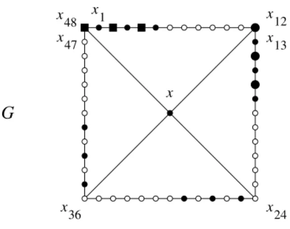
Figure 1: Graph G in Proposition 9, for r = 6 and k = 4. Squares and circles, white or black, small or large, are vertices. The 19 black vertices constitute a 6-identifying code in G.
Remark preceding the proof. The lower bound (4) is equivalent to n/4 when n increases with respect to r. An open question is whether this can be improved. The lower bound (5) is equivalent to 2, but will be strongly improved in Proposition 15.
Proof of Proposition 9. Let r ≥ 2 be an even integer, and n be an (even) integer such that n = k · 2r, k ≥ 2; let Gx= Cn= x1x2. . . xn be the cycle of
length n and G be the graph obtained from Gx by adding the vertex x and
linking it to the k vertices xj·2r, 1 ≤ j ≤ k. See Figure 1, which illustrates
the case r = 6, k = 4, n = 48 and G has 49 vertices.
We know by Theorem 8 that γr(Gx) = n2, and we claim that
γr(G) ≤ 1 + (k + 2)
n 4k =
n
4 + r + 1,
from which (4) and (5) follow. Proving this claim, by exhibiting an r-identifying code for G, is tedious and of no special interest; therefore, we content ourselves with showing how it works in the case r = 6, n = 48, hoping that this will help the reader to gain an insight into the general case. We consider a first set
S = {x, x1, x3, x5, x13, x15, x17, x25, x27, x29, x37, x39, x41},
see the small black circles in Figure 1. It is now quite straightforward to observe that the pairs {x48, x1}, {x2, x3} and {x4, x5} are pairs of (G, S,
6)-twins, as well as {x12, x13}, {x14, x15}, {x16, x17}, {x24, x25}, {x26, x27},
{x28, x29}, {x36, x37}, {x38, x39} and {x40, x41}, for reasons of symmetry,
and that they are the only ones.
Let us consider the first three pairs, {x48, x1}, {x2, x3}, {x4, x5}. Using
x16, x14 and x12 (see the large black circles), and these three vertices also
6-separate the other pairs of (G, S, 6)-twins, except for {x12, x13}, {x14, x15},
{x16, x17}. These three pairs can however be 6-separated by three more
codewords, for instance x4, x2 and x48, see the black squares in Figure 1.
Now the code
C = S ∪ {x12, x14, x16, x48, x2, x4}
is 6-identifying in G and has 1 + (4 × 3) + (2 × 3) = 19 codewords. In the general case,
S = {x} ∪ {x1+j·2r, x3+j·2r, . . . , xr−1+j·2r: 0 ≤ j ≤ k − 1},
there are k × r2 pairs of (G, S, r)-twins, and C can be chosen, for instance, as
C = S ∪ {xn, x2, . . . , xr−2} ∪ {x2r, x2r+2, . . . , x2r+(r−2)},
which shows that the cardinality of C is 1 + (k ×r 2) + (2 × r 2) = 1 + (k + 2) n 4k, and so γr(G) ≤ 1 + (k + 2)4kn. △
Conclusion 10 When r is even, Proposition 9 gives pairs of connected graphs proving that γr(Gx) − γr(G) can be, asymptotically, as large as
ap-proximately n 4.
• (ii) Case of a connected graph Gx and r ≥ 3, r odd
Proposition 11 There exist two (connected) r-twin-free graphs G and Gx,
with n + 1 and n vertices respectively, such that γr(Gx) − γr(G) ≥ n(3r − 1) 12r − r, (6) γr(Gx) γr(G) ≥ 6nr n(3r + 1) + 12r2. (7)
Remark preceding the proof. An open question is whether the first lower bound, which is equivalent to n(3r−1)12r when r is fixed and n goes to infinity, can be improved. The second lower bound, equivalent to 3r+16r , will be improved in Proposition 15.
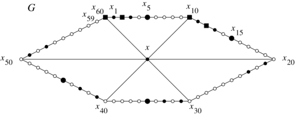
Proof of Proposition 11. Let r ≥ 3 be an odd integer, and n be an (even) integer such that n = k · 2r, where k ≥ 3 is a multiple of 3; let Gx = Cn=
x1x2. . . xn be the cycle of length n and G be the graph obtained from Gx
by adding the vertex x and linking it to the k vertices xj·2r, 1 ≤ j ≤ k.
See Figure 2, which illustrates the case r = 5, k = 6, n = 60 and G has 61 vertices.
x 1 x 20 x 50 x 60 x 59 x 15 x 5 x10 x 30
G
x x 40Figure 2: Graph G in Proposition 11, for r = 5 and k = 6. Squares and circles, white or black, small or large, are vertices. The 21 black vertices constitute a 5-identifying code in G.
We know by Theorem 8 that γr(Gx) = n2, and we claim that
γr(G) ≤
n 4 +
n 12r + r,
from which (6) and (7) follow. Again, proving this claim is of no interest here, and we just show how it works in the case r = 5, n = 60. We consider a first set
S = {x, x1, x3, x11, x13, x21, x23, x31, x33, x41, x43, x51, x53},
see the small black circles in Figure 2. It is straightforward to see that only the following sets of (G, S, 5)-twins exist:
• (i) {x, x10, x20, x30, x40, x50, x60},
• (ii) {x59, x1, x2} together with the five symmetrical sets {x9, x11, x12}, . . .,
• (iii) {x3, x4} together with the five symmetrical sets {x13, x14}, . . .
The first two cases are annoying and will be “expensive” because they present symmetries with respect to x. Define the set T as follows:
T = S ∪ {x5, x15, x35, x45},
see the large black circles in Figure 2. Now in Case (i), all the vertices are 5-separated by the vertices in T \ S, and so are x59 on the one hand and
x1, x2 on the other hand, as well as their symmetrical counterparts from
Case (ii). The remaining pairs of (G, T , 5)-twins are {x1, x2}, {x3, x4} and
the 10 pairs obtained by symmetry. As in the proof of Proposition 9, these handle very economically: the vertex x605-separates the 5 pairs {x13, x14},
. . . , {x53, x54}, and so does x2 for {x11, x12}, . . . , {x51, x52}; finally, {x1, x2}
and {x3, x4} can be 5-separated, for instance, by x10and x12, see the black
squares in Figure 2:
is a 5-identifying code in G and has 1 + (6 × 2) + (4 × 1) + (2 × 2) = 21 codewords. In the general case,
S = {x} ∪ {x1+j·2r, x3+j·2r, . . . , xr−2+j·2r : 0 ≤ j ≤ k − 1}
contains 1 + (k ×r−12 ) vertices; then
T = S ∪ {xr+j·2r : 0 ≤ j ≤ k − 1, j not congruent to 2 modulo 3}
contains |S| +2k3 elements, and finally we take
C = T ∪ {xn, x2, . . . , xr−3} ∪ {x2r, x2r+2, . . . , x2r+(r−3)},
which shows that
γr(G) ≤ 1 + (k × r − 1 2 ) + 2k 3 + (2 × r − 1 2 ) = n 4 + n 12r + r. △ Conclusion 12 When r ≥ 3 and r is odd, Proposition 11 gives pairs of connected graphs proving that γr(Gx) − γr(G) can be, asymptotically, as
large as approximately n(3r−1)12r .
If we do not require to consider a connected graph Gx, then we can
ob-tain a larger difference or ratio than in (4)-(7), we need consider only one case, whatever the parity of r is, and moreover the construction is easy to understand; see next paragraph.
• (iii) Case of a disconnected graph Gx and r ≥ 2, r even or odd
Proposition 13 There exist two graphs G and Gx, with p(2r + 1) + 1 and
n = p(2r + 1) vertices respectively, such that γr(Gx) − γr(G) ≥ n(2r − 2) 2r + 1 − 2r, (8) γr(Gx) γr(G) ≥ nr n + 4r2+ 2r. (9)
Remark preceding the proof. Can the first lower bound, equivalent to
n(2r−2)
2r+1 , be improved? The second bound, equivalent to r, is still improved
in Proposition 15.
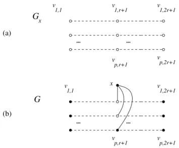
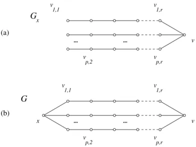
Proof of Proposition 13. Let r ≥ 2 and p ≥ 3 be integers; the graph Gx consists of p copies of the path P2r+1, and G is obtained by adding the
vertex x and linking it to all the middle vertices of the path copies, see Figure 3. We claim that: (a) γr(Gx) = 2pr and (b) γr(G) ≤ 2p + 2r, from
v 1,1 v 1,2r+1 v 1,r+1 v p,2r+1 v 1,1 (a) (b) ... ... ... ... G x p,r+1 v p,r+1 v v x G p,2r+1 v 1,2r+1
Figure 3: The graphs Gx and G in Proposition 13.
Proof of (a). The result comes from the obvious fact that γr(P2r+1) = 2r.
Proof of (b). It is not difficult to check that
C = {x} ∪ {vi,1, vi,2r+1: 1 ≤ i ≤ p − 1} ∪ {vp,j : 1 ≤ j ≤ 2r + 1}
(see the black circles in Figure 3) is indeed r-identifying in G. Note however that, for simplicity, we chose to give the bound 2p + 2r, when actually, with a little more care, 2p + 2r − 3 can be reached, which would improve only
slightly on (8) and (9). △
Conclusion 14 Proposition 13 gives pairs of graphs (G, Gx), where Gx is
not connected, proving that γr(Gx) − γr(G) can be, asymptotically, as large
as approximately n(2r−2)2r+1 .
Finally, we give a construction (obtained with connected graphs) with a ratio γr(Gx)/γr(G) arbitrarily large, but where the difference γr(Gx) − γr(G) is
not as large as in (4) and (6).
Proposition 15 Let k ≥ 2 be an arbitrary integer. There exist two (con-nected) r-twin-free graphs G and Gx, where G has 2rk +r⌈log2(k +1)⌉+r +1
vertices, such that
γr(Gx)
γr(G)
≥ k
r⌈log2(k + 1)⌉ + r + 1. (10)
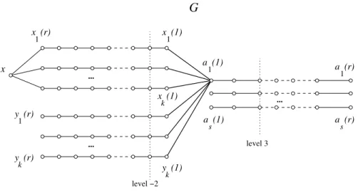
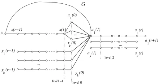
Proof. The construction is a straigthforward generalization to any r ≥ 2 of the one used in the proof of Proposition 4, see Figure 4; the basic idea is similar, but the implementation becomes somewhat more involved.
level 3 a (1) 1 1 y (r) ... ... G k x (1) ... k y (1) s 1 a (r) a (r) a (1) s level −2 1 x (1) x (r) 1 k y (r) x
Figure 4: A partial representation of the graph G in Proposition 15: more edges exist between the vertices xi(1) and yi(1) on the one hand, and the
vertices aj(1) on the other hand. The case r = 1 can be used to illustrate
Proposition 4.
We consider, for each i between 1 and k, the paths xi(1)xi(2) . . . xi(r),
and yi(1)yi(2) . . . yi(r). We need also some auxiliary vertices. Denoting
again s = ⌈log2(k + 1)⌉ + 1, for each j = 1, 2, . . . , s, we consider the path aj(1)aj(2) . . . aj(r); we denote the set of these sr auxiliary vertices by A.
We say that the vertices xi(−h), yi(−h) and aj(h) are on the h-th level (cf.
Figure 4).
We now imitate the proof of Proposition 4, and for each i ∈ {1, . . . , k} choose a unique nonempty subset Aiof the set {a2(1), . . . , as(1)} and connect
xi(1) and yi(1) by an edge to the vertices aj(1) for which j ∈ {1} ∪ Ai.
In the resulting graph Gx, we first take all the vertices in A as codewords.
Then we observe that for an arbitrary, unknown vertex v,
• Br(v) contains at least two vertices aj(r) if v is on the level -1;
• Br(v) does not contain any vertices aj(r) if v is on the h-th level for
some h ≤ −2; and
• Br(v) contains exactly one aj(r) if v ∈ A.
From the last case we see that we can uniquely tell whether or not v ∈ A simply by looking which vertices of A are in Br(v). We can in fact do even
more: if j is the only index for which aj(r) is in Br(v), then v is one of
the vertices aj(h) for some h = 1, 2, . . . , r. We know that aj(1) is connected
to at least one xi(1) (as we chose s to be as small as possible) and xi(1)
is connected to at least one aj′(1) with j′ 6= j. Then exactly r − h of the
Assume now that we already know that v /∈ A. Let h be the highest level for which some aj(h) belongs to Br(v). Then v must be one of the vertices
xi(r + 1 − h) or yi(r + 1 − h), and moreover, we can uniquely tell i by looking
at the indices j for which aj(h) belong to Br(v), because by the construction
{j : aj(h) ∈ Br(v)} = {1} ∪ Ai (as we can only reach these vertices from v
by going from v to xi(1) or yi(1) and from it directly to those aj(1) to which
xi(1) or yi(1) was connected to by an edge).
In conclusion, by only looking at which auxiliary vertices are in Br(v)
we can ”almost” identify v: we find indices i and m such that v is either xi(m) or yi(m). This implies that the graph is clearly r-twin-free. Indeed, if
all the vertices are in the code, then the only remaining task, i.e., separating each xi(m) from yi(m), becomes easy: if xi(r) is in Br(v) then v = xi(m);
if not then v = yi(m).
Moreover, every r-identifying code must contain at least one element of the set {xi(1), xi(2), . . . , xi(r), yi(1), yi(2), . . . , yi(r)}: otherwise we cannot
r-separate xi(1) and yi(1). Consequently, any r-identifying code in this
graph has size at least k.
We now add one more vertex x, and connect it by an edge to each xi(r). We claim that the vertex x together with all the vertices in A form
an r-identifying code. By the construction, the set Br(v), v 6= x, contains
exactly the same vertices of A as before adding the vertex x (and the set Br(x) contains none), so the only thing to check is that xi(m) and yi(m)
can now be r-separated: but this is indeed done by x. △
Remark. In terms of n = 2rk + r⌈log2(k + 1)⌉, the lower bound (10) can be approximated by n
2r2log
2n and is open to improvements.
Conclusion 16 Proposition 15 gives pairs of (connected) graphs proving that γr(Gx)/γr(G) can be, asymptotically, as large as approximately 2r2logn
2n.
Then we turn to examples where γr(G) − γr(Gx) is arbitrarily large. Note
that we obtain this result with connected graphs.
Proposition 17 There exist two (connected) r-twin-free graphs Gx and G,
with n = pr + 1 and pr + 2 vertices respectively, such that γr(Gx) = p + 2r − 3 =
n + 2r2− 3r − 1
r and γr(G) = r(p − 1) + 1 = n − r, where p is any integer greater than or equal to 3.
Proof. Let r ≥ 2 and p ≥ 3 be integers; before defining G, we describe Gx
in the following informal way, illustrated in Figure 5(a): Gx consists of
p copies of the path Pr, and in each copy the last vertex is linked to v. This
graph has n = pr + 1 vertices. Next, we construct the graph G consisting of Gx to which we add one vertex x, linked to each first vertex of all the
v 1,1 v p,r v p,2 v 1,r x v v p,r v p,2 v v 1,r v 1,1 (a) (b) ... ... ... ... G Gx
Figure 5: The graphs Gx and G in Proposition 17.
copies of Pr. See Figure 5(b). We claim that: (a) γr(Gx) = p + 2r − 3, and
(b) γr(G) = r(p − 1) + 1, from which (13) and (14) follow.
Proof of (a). The code
C = {v1,i : 2 ≤ i ≤ r} ∪ {v2,i: 1 ≤ i ≤ r} ∪ {vj,1: 3 ≤ j ≤ p},
i.e., the code consisting of all the vertices of the first two copies of Pr,
except v1,1, and the first vertex of each of the following copies, is r-identifying
in Gx; this it is straightforward to check. So γr(Gx) ≤ (r − 1) + r + (p − 2) =
p + 2r − 3. We now prove that γr(Gx) ≥ p + 2r − 3. The following two
observations will be useful. For 1 ≤ i ≤ p and 2 ≤ k ≤ r, we have:
BGx,r(vi,r−k+1)∆BGx,r(vi,r−k+2) = {vj,k : 1 ≤ j ≤ p, j 6= i}, (11)
where ∆ stands for the symmetric difference, and for 1 ≤ i < j ≤ p:
BGx,r(vi,r)∆BGx,r(vj,r) = {vi,1, vj,1}. (12)
The consequences are immediate. First, in order to have the vertices vi,r,
1 ≤ i ≤ p, pairwise r-separated in Gx, we see by (12) that we need at least
p − 1 codewords among the p vertices vi,1; second, for k fixed between 2
and r, we see, using (11), that we need at least two codewords among the p vertices vi,k. So γr(Gx) ≥ (p − 1) + 2(r − 1) = p + 2r − 3, and Claim (a)
is proved.
Proof of (b). Note that in G, for i and j such that 1 ≤ i < j ≤ p, the set of vertices
forms the cycle C2r+2, which is r-twin-free and is denoted by C(i, j). On
such a cycle, we say that the vertex z is the opposite of the vertex y if z is the (only) vertex at distance r + 1 from y.
We claim that, for k fixed between 1 and r, among the p vertices vi,k, at
least p − 1 of them belong to any r-identifying code C in G. Indeed, assume on the contrary that two vertices, say v1,k and v2,k, are not in C; then their
opposite vertices in C(1, 2), v2,r−k+1 and v1,r−k+1 respectively, cannot be
r-separated by C.
Finally, the fact that BG,r(v)∆BG,r(x) = {v, x} shows that v or x belong
to C, and finally γr(G) ≥ (p − 1)r + 1. On the other hand,
{v} ∪ {vi,k : 2 ≤ i ≤ p, 1 ≤ k ≤ r}
is an r-identifying code in G, with size (p − 1)r + 1, thus Claim (b) is proved. Observe that this code contains all the vertices in G, except the r+1 vertices
x and v1,k, 1 ≤ k ≤ r. △
Note that we could have contented ourselves with the inequalities γr(Gx) ≤
p + 2r − 3 and γr(G) ≥ r(p − 1) + 1, so as to obtain γr(G) − γr(Gx) ≥
p(r − 1) − 3r + 4 and γr(G)
γr(Gx) ≥
r(p−1)+1 p+2r−3 .
Remark. The difference
γr(G) − γr(Gx) = p(r − 1) − 3r + 4
can be made arbitrarily large; in terms of n, the number of vertices of Gx,
we can see that we have:
γr(G) − γr(Gx) =
(n − 3r)(r − 1) + 1
r , (13)
which is equivalent to n(r−1)r when r is fixed and n goes to infinity. As far as the ratio given by Proposition 17 is concerned, we have:
γr(G)
γr(Gx)
= r(n − r)
n + 2r2− 3r − 1, (14)
which is equivalent to r when we increase n. This can be improved, with a ratio which becomes arbitrarily large; again, it so happens that the graphs are connected:
Proposition 18 Let k ≥ 2 be an arbitrary integer.
There exist two (connected) 2-twin-free graphs G and Gx, where G has 3k +
2⌈log2(k + 2)⌉ + 4 vertices, such that γ2(G)
γ2(Gx)
≥ k
Let r ≥ 3. There exist two (connected) r-twin-free graphs G and Gx, where
G has (r + 1)k + r⌈log2(k + 2)⌉ + 2r + 1 vertices, such that γr(G)
γr(Gx) ≥
k
r⌈log2(k + 2)⌉ + r + 3. (16)
Proof. We first deal with the general case r ≥ 3. We construct the graph G for a given k ≥ 2 in the following way, see Figure 6: G consists of the paths xi(0)x(1)x(2) . . . x(r−2)x(r−1)x and yi(0)yi(1) . . . yi(r−1), for i = 1, . . . , k,
of the path a1(1) . . . a1(r + 1), of the paths aj(1) . . . aj(r) for j = 2, . . . , s,
where s = 1 + ⌈log2(k + 2)⌉, plus the edge xa1(1) and the following edges,
joining exclusively the vertices xi(0) and yi(0) on the one hand, and the
vertices aj(1) on the other hand: for each i we choose a unique nonempty
proper subset Ai of the set A = {2, 3, . . . , s}, and connect every xi(0) and
every yi(0) to every vertex aj(1) for which j ∈ Ai. Moreover, we connect
every xi(0) and every yi(0) to a1(1). The sets Ai can indeed be chosen in
this way, because there are 2s−1 − 2 proper nonempty subsets of A, and s − 1 = ⌈log2(k + 2)⌉. Without loss of generality, we can choose the sets Ai in such a way that each aj(1) has degree at least two, and so the graph
constructed is connected, as will be Gx.
We say that the vertices x(−h), xi(−h), yi(−h) and aj(h) are on the
h-th level, cf. Figure 6 (and x is not given any level). Let A = {aj(h) : 1 ≤ j ≤ s, 1 ≤ h ≤ r} ∪ {a1(r + 1)}.
Let us first consider Gx, and let C = A ∪ {x1(0), x(r − 1)}. We show that
C is r-identifying, so that γr(Gx) ≤ sr + 3. The argument is very similar to
the first part of the proof of Proposition 15: let v be an arbitrary, unknown vertex in Gx.
If v belongs to A, then v is r-covered by exactly one codeword aj(r),
whereas every vertex of level 0 is r-covered by at least two codewords of level r, and no vertex with negative level is r-covered by any codeword of level r; if v ∈ A is r-covered by aj(r), we know moreover that v = aj(h)
for some h between 1 and r + 1. If h < r, then h is given by the highest level ℓ of any codeword aj′(ℓ) r-covering aj(h), with j′ 6= j (such a j′ exists
because aj(1) is connected to at least one xi(0), which in turn is connected
to at least one aj′(1)). If j 6= 1 and h = r, then h is given by the fact that
no codeword aj′(ℓ) (j′6= j) r-covers aj(h). And if j = 1 and h ∈ {r, r + 1},
then the codeword x1(0) tells whether h = r or h = r + 1. This means that
we can determine first that v ∈ A, then on which path and at which level it is located.
If v /∈ A, then its level can be determined by the highest level, say ℓ, of the codewords in A which r-cover it. Then the codeword x(r − 1) tells if v is of type x or y; and finally, if v = xi(0) or v = yi(h) for some h between 0
1 k ... G k x (0) 1 y (r−1) ... k y (r−1) s a (r) a (1) s 1 a (r+1) x x(r−1) x(1) level 2 level −1 ... y (0) x (0) 1 level 0 a (r) 1 a (1)
Figure 6: A partial representation of the graph G in Proposition 18, in the general case r ≥ 3: more edges exist between the vertices xi(0) and yi(0) on
the one hand, and the vertices aj(1) on the other hand.
aj(ℓ) ∈ Br(v), because by the construction {j : aj(ℓ) ∈ Br(v)} = {1} ∪ Ai.
This ends the study of Gx.
We now consider the graph G, and prove that it is r-twin-free. Com-paring with the previous graph Gx, it is still true that every vertex in A
is r-covered by exactly one vertex aj(r), whereas every vertex of level 0 is
r-covered by at least two vertices of level r, and no vertex with negative level is r-covered by any vertex of level r – and note that x is r-covered by exactly one aj(r), namely a1(r); it is still true that no two vertices inside A
are r-twins, that one vertex in A and one vertex of type y or x (except maybe x itself) are not twins, and that no two vertices of type y are r-twins; also, thanks to the vertices yi(r −1), no vertex of type y can be r-twin
with a vertex of type x; but we have to see what happens with the vertices of type x between themselves, and with the vertex x and one vertex in A.
Now x is not r-twin with any aj(h), j > 1, thanks to aj(r), and not either
with any a1(h), thanks to a1(r + 1) – note in particular that a1(r + 1) is
the only vertex r-separating x and a1(2). Assume finally that v is of type x,
v 6= x. If v = xi(0) for some i, the set of indices j for which aj(r) ∈ Br(v)
equals {1} ∪ Ai, has size at least two, and identifies v. So assume that v is
not on level 0, and denote by h ∈ {1, 2, . . . , r − 1} the largest level for which at least one aj(h) belongs to Br(v). If the only shortest path between v
and a1(1) goes via x, then {j : aj(h) ∈ Br(v)} = {1}; if there is a shortest
path between v and a1(1) that goes via one (and hence all) xi(0), then
{j : aj(h) ∈ Br(v)} = {1, 2, . . . , s}: in both cases, h uniquely identifies v.
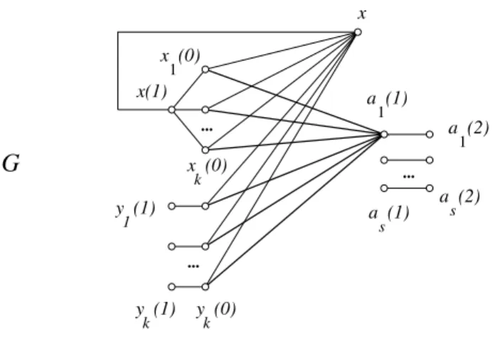
k y (1) k y (0) 1 y (1) a (1) 1 a (1) s a (2) s a (2) 1 x (0) 1 k x (0) ... ... G x(1) ... x
Figure 7: A partial representation of the graph G in Proposition 18, in the particular case r = 2: more edges exist between the vertices xi(0) and yi(0)
on the one hand, and the vertices aj(1) on the other hand.
a given i between 1 and k, it is easy to see that we have:
Br(yi(0)) = Br(xi(0)) ∪ {yi(r − 1)}, (17)
where the right-hand side is a disjoint union; this shows that any r-identifying code in G contains at least k elements, and ends the case r ≥ 3. Note that if we had considered this construction for r = 2, then (17) would not be true, since x(1) would be in B2(xi(0)) \ B2(yi(0)).
When r = 2, the previous construction does not work, as we have just seen, but the following does: the x-paths are again xi(0)x(1)x, and the y-paths
are yi(0)yi(1) as before; the vertex a1(3) is removed, and, keeping all the
edges between the vertices of level 1 in A and the vertices of level 0 as before, we add all the edges between x and the vertices of level 0; see Figure 7.
It is then rather straightforward, using the same kind of argument as in the general case, to check that C = {aj(h) : 1 ≤ j ≤ s, 1 ≤ h ≤ 2} ∪ {x(1)}
is 2-identifying in Gx, that G is 2-twin-free, and that any 2-identifying code
in G needs at least k codewords. △
Remark. In terms of n = (r + 1)k + r⌈log2(k + 2)⌉, the approximate order of G and Gx, we can approximate the lower bounds in (15) and (16) by
n
r(r+1) log2n. Again, can the bounds given in (13), (15) and (16) be
signifi-cantly improved?
Conclusion 19 When r ≥ 2, Propositions 17 and 18 provide pairs of graphs proving that γr(Gx) − γr(G) can be, asymptotically, as small as
approxi-mately −n(r−1)r , and γr(Hx)
γr(H) can be, asymptotically, as small as approximately
r(r+1) log2n
5
General conclusion
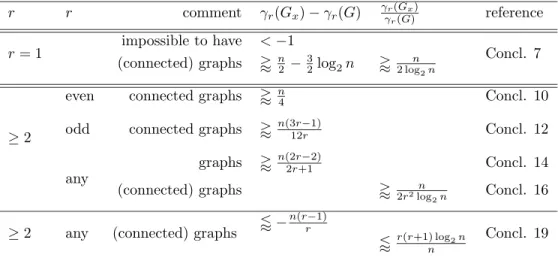
Table 1 recapitulates the results obtained in the previous sections, using in particular the Conclusions 7, 10, 12, 14, 16 and 19; these are stated for n large with respect to r, where n is the approximate order of G or of Gx; when using ' X (respectively, / X), we mean that we have a lower
bound (respectively, an upper bound), for the difference or ratio, which is approximately X . We only consider the difference γr(Gx) − γr(G) and the
ratio γr(Gx) γr(G). r r comment γr(Gx) − γr(G) γr(Gx) γr(G) reference impossible to have < −1 r = 1 (connected) graphs 'n 2 − 3 2log2n '2 logn2n Concl. 7 ≥ 2
even connected graphs 'n
4 Concl. 10
odd connected graphs 'n(3r−1)12r Concl. 12
any
graphs 'n(2r−2)2r+1 Concl. 14
(connected) graphs ' n
2r2log2n Concl. 16
/ −n(r−1)r
≥ 2 any (connected) graphs
/r(r+1) log2n
n
Concl. 19
Table 1: The difference γr(Gx) − γr(G) and ratio γ
r(Gx)
γr(G), as functions of n
Part II: Addition and deletion of one edge
This part is organized as follows. Section 6 is devoted to the case r = 1; here, the difference γ1(Ge)−γ1(G) must lie between −2 and +2. Then in the
beginning of Section 7, we study how small γr(Ge)−γr(G) and γr(Ge)/γr(G)
can be for any r ≥ 2, and it so happens that the graphs we use are connected (Corollary 27 for r ≥ 5 and Proposition 28 for r ∈ {2, 3, 4}); finally, we study how large these difference and ratio can be, for r ≥ 3 in Corollary 29 and for r = 2 in Proposition 30 (in both cases, the graphs can be made connected).
A conclusion recapitulates our results in a Table.
6
The case r = 1
The difference γ1(Ge) − γ1(G) can vary only inside the set {−2, −1, 0, 1, 2}
(Theorem 24), and these five values can be reached (Examples 21, 23 and 25). We first study how small γ1(Ge) − γ1(G) can be. Putting the cart before
the horse, in the next theorem we first define Ge, and only then, G.
Theorem 20 Let Ge = (V, Ee) be a 1-twin-free graph with at least four
vertices, let x and y be two distinct vertices in V such that e = xy /∈ Ee,
and let G = (V, E) with E = Ee∪ {xy}. Assume that G is also 1-twin-free.
If Ceis a 1-identifying code in Ge, then there exists a 1-identifying code C
in G with
|C| ≤ |Ce| + 2.
As a consequence, we have:
γ1(Ge) − γ1(G) ≥ −2. (18)
Proof. Since we add an edge when going from Ge to G, all vertices remain
1-covered, in G, by at least one codeword in Ce.
Since we only add the edge xy, only the balls of x and y are modified in G. As a consequence, only the following pairs are possible (G, Ce, 1)-twins:
• x and y, • x and u with u 6= x, u 6= y, • y and v with v 6= x, v 6= y. Moreover, x and u′ , with u′ 6= u, u′ 6= x, u′ 6= y, cannot be (G, Ce, 1)-twins
since this would imply, by Lemma 1, that u and u′
are (G, Ce, 1)-twins, hence
(Ge, Ce, 1)-twins, which would contradict the fact that Ce is 1-identifying
in Ge. The same is true for y and v′, with v′ 6= v, v′ 6= x, v′ 6= y. So at most
three pairs of (G, Ce, 1)-twins can appear.
Similarly, if these three pairs of (G, Ce, 1)-twins all do appear, then u
and v are (G, Ce, 1)-twins, which leads to the same contradiction, unless
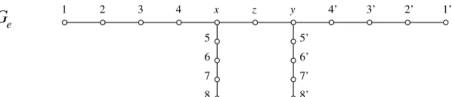
x z y 4’ 3’ 2 1 3 2’ 1’ 5 6 7 8 5’ 6’ 7’ 8’ e G 4
Figure 8: Graph Ge in Example 21.
codeword c1 1-separating x and u by, say, 1-covering x and not u. If c1
1-covers y, then c1 also 1-separates y and u; if c1 does not 1-cover y, then
c1 also 1-separates y and x. In both cases, we are left with one pair of
vertices not yet 1-separated by a codeword, which we can do with a second additional codeword c2. Now C = Ce∪ {c1, c2} is 1-identifying in G, and it
has |Ce| + 2 elements.
When at most two pairs of (G, Ce, 1)-twins appear, then obviously with
at most two more codewords added to Ce we can 1-separate them. △
Note that we made no assumption on the connectivity of Ge. The following
example shows that graphs Ge and G with γ1(G) = γ1(Ge) + 2 do exist; we
do not know if this is the smallest possible example.
Example 21 Let Ge= (V, Ee) be the graph represented in Figure 8, and G
the graph obtained by adding the edge e = xy. We claim that: (a) γ1(Ge) ≤
10 and (b) γ1(G) ≥ 12, which by (18) implies that γ1(G) = 12 = γ1(Ge) + 2.
Proof of (a). It is quite straightforward to check that Ce= {1, 3, x, 6, 8, 8′,
6′
, y, 3′
, 1′} is 1-identifying in G
e. Hence γ1(Ge) ≤ 10.
Proof of (b). Let C be a 1-identifying code in G. Because 1 and 2 must be 1-separated by C, we have 3 ∈ C; and because 1 must be 1-covered by at least one codeword, we have 1 ∈ C or 2 ∈ C. Similarly, C contains 6, 6′
, 3′
and at least one element in each of the 2-sets {7, 8}, {8′
, 7′
} and {2′
, 1′
}, which amounts to eight codewords.
With simple arguments, we obtain the following fact: • there are at least three codewords in {1, 2, 3, 4, x}. The same is true for {x, 5, 6, 7, 8}, {y, 5′
, 6′ , 7′ , 8′ } and {y, 4′ , 3′ , 2′ , 1′ }. So, if neither x nor y belongs to C, there are at least 3 × 4 = 12 codewords, and we are done.
If, on the other hand, both x and y belong to C, then we have already ten codewords, and still x, y and z are not 1-separated by any codeword; this will require two additional codewords, and again, |C| ≥ 12.
If we assume finally, without loss of generality, that x ∈ C and y /∈ C, then we have already chosen (3 × 2) + 5 = 11 codewords: three in each of the
sets {4′, 3′, 2′, 1′} and {5′
, 6′, 7′, 8′}, one in each of the sets {1, 2} and {7, 8}, plus 3, 6 and x; still, x and z are not 1-separated by any codeword, so again we need at least twelve codewords, which proves Claim (b). △ Next, we establish how large γ1(Ge) − γ1(G) can be.
Theorem 22 Let G = (V, E) be a 1-twin-free graph with at least four ver-tices, let x and y be two vertices in V such that e = xy ∈ E, and let Ge= (V, Ee) with Ee= E \ {xy}. Assume that Ge is also 1-twin-free.
If C is a 1-identifying code in G, then there exists a 1-identifying code Ce
in Ge with
|Ce| ≤ |C| + 2.
As a consequence, we have:
γ1(Ge) − γ1(G) ≤ 2. (19)
Proof. We assume that C is not 1-identifying in Ge anymore, otherwise we
are done. There can be two reasons why C is not 1-identifying:
1) at least one of the two vertices x and y, say x, is not 1-covered by any codeword anymore:
BGe,1(x) ∩ C = ∅ = (BG,1(x) \ {y}) ∩ C,
which implies that BG,1(x) ∩ C = {y}, y ∈ C and x /∈ C; we see that in this
case y is still 1-covered by a codeword, namely itself.
If meanwhile all vertices remain 1-separated by C in Ge, then C ∪ {x}
is 1-identifying in Ge. But this first reason can go along with the second
reason:
2) (Ge, C, 1)-twins appear;
because only the edge xy is deleted when going from G to Ge, and similarly
to the proof of Theorem 20, only the following pairs can be (Ge, C, 1)-twins:
• x and y,
• x and u with u 6= x, u 6= y, • y and v with v 6= x, v 6= y.
If x and y are (Ge, C, 1)-twins, this means that
BGe,1(x) ∩ C = BGe,1(y) ∩ C,
which implies that x /∈ C, y /∈ C, and so
BG,1(x) ∩ C = BG,1(y) ∩ C,
contradicting the fact that C is 1-identifying in G. Assume next that x and u are (Ge, C, 1)-twins. Then
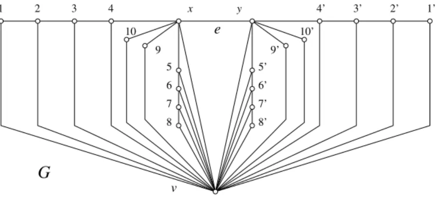
4’ 3’ 2 1 3 2’ 1’ 5 6 7 8 5’ 6’ 7’ 8’ x e 9’ 9 10 10’ G v 4 y
Figure 9: Graph G in Example 23. and so
y ∈ C and BGe,1(x) ∩ C = (BG,1(x) ∩ C) \ {y}.
If x and u are the only (Ge, C, 1)-twins, then with two more codewords we
can both 1-cover x if necessary and 1-separate x and u in Ge. The same
argument would work if y and v were the only (Ge, C, 1)-twins. So we assume
that x and u, and y and v are (Ge, C, 1)-twins. This implies that both x
and y are codewords, each 1-covered by itself. All there is left to do is to 1-separate two pairs of (Ge, C, 1)-twins in Ge, which can be done using two
more codewords. △
Note that we made no assumption on the connectivity of G and Ge. The
following example shows that (connected) graphs G and Ge with γ1(Ge) =
γ1(G) + 2 exist.
Example 23 Let G = (V, E) be the graph represented in Figure 9, and Ge
the graph obtained by deleting the edge xy. We claim that: (a) γ1(G) ≤ 12
and (b) γ1(Ge) ≥ 14, which by (19) will imply that γ1(Ge) = 14 = γ1(G) +2.
Proof of (a). It is quite straightforward to check that C = {1, 3, x, 6, 8, 9, 9′ , 8′ , 6′ , y, 3′ , 1′} is 1-identifying in G. Hence γ 1(G) ≤ 12.
Proof of (b). Let Ce be an optimal 1-identifying code in Ge, not
contain-ing v: thanks to Lemma 3, we know that this is possible. We are gocontain-ing to show that the left part of the graph Ge, consisting of the vertices 1 to 10
and x, requires at least seven codewords.
As in Example 21, we have 3 ∈ Ce, 6 ∈ Ce, and, because v /∈ Ce, Ce also
contains at least one element in each of the 2-sets {1, 2} and {7, 8}, which amounts to four codewords.
As in Example 21, we also have that:
and three codewords in {x, 5, 6, 7, 8}. So, if x /∈ Ce, there are, because of 9
and 10, at least 3 + 3 + 2 = 8 codewords, and we are done. We now assume that x ∈ Ce, so that we have already taken five codewords. One more
code-word is not sufficient to 1-separate both 9 and 10, 9 and x, and 10 and x.
This proves Claim (b), by symmetry. △
By Theorems 20 and 22, we have the following result.
Theorem 24 Let G1 and G2 be two 1-twin-free graphs, with same vertex
set and differing by one edge. Then
γ1(G1) − 2 ≤ γ1(G2) ≤ γ1(G1) + 2.
As a consequence, if for instance γ1(G1) ≤ a and γ1(G2) ≥ a + 2, then
γ1(G1) = a and γ1(G2) = a + 2. △
We conclude the case r = 1 by mentioning that pairs of graphs G and Ge
such that γ1(Ge) − γ1(G) = 0 or γ1(Ge) − γ1(G) = ±1 exist.
Example 25 We give simple examples with (a) γ1(Ge) − γ1(G) = −1 and
(b) γ1(Ge) − γ1(G) = 1, omitting the easy case when the difference is 0.
(a) Let Ge = P9 = x1x2. . . x9, and add the edge {x3, x5} in order to
obtain G. It is known ([3, Th. 3]) that γ1(P9) = 5, and it is easy to see that
γ1(G) = 6, so γ1(Ge) − γ1(G) = −1.
(b) Let Ge be the graph consisting of P1 and P4, and G be the graph
obtained by adding an edge between one extremity of P4 and the vertex of P1,
so that G = P5. We have γ1(P1) = 1, γ1(P4) = 3, and γ1(P5) = 3, which
shows that γ1(Ge) − γ1(G) = 1. △
7
The case r ≥ 2
We now give our central result, Theorem 26. It describes graphs for which we delete edges and/or vertices, because we think that it is interesting to have such a ”mixed construction”, cf. Introduction and the forthcoming paper [6]. It also presents the remarkable feature that, starting from the graph G and performing two consecutive deletions, we first decrease the function γr, then
increase it. The consequences of this result for edge deletion are detailed in Corollaries 27 and 29, and are extended in Propositions 28 and 30. For simplicity, we give constructions where two of the graphs, namely
(G \ e) \ f and (G \ u) \ f,
are disconnected, but the remarks after the proofs of Corollary 29 and of Proposition 30 show an easy way to have connected graphs, with a slightly different result, when needed. Since we estimate the value of γr for all these
graphs, this means that all are r-twin-free, a fact not stated explicitly in the theorem.
... ... G x(r−2) v=x(r−1) f e ... k x (r−3) k x (0) 1 y (r−1) ... k y (r−1) k y (0) x (0) 1 s 1 a (r) a (r) u=x(r) level 2 a (1) s level −1 r x (r−3) a (1) 1 level 5− 1
Figure 10: A partial representation of the graph G in Theorem 26: more edges exist between the vertices xi(0) and yi(0) on the one hand, and the
vertices aj(1) on the other hand.
Theorem 26 Let k ≥ 2 be arbitrary and r ≥ 5. There exists a graph G with (2r − 2)k + r⌈log2(k + 2)⌉ + r + 3 vertices with the following properties:
(i) γr(G) ≥ k.
(ii) There is an edge e of G such that γr(G \ e) ≤ 1 + r + r⌈log2(k + 2)⌉.
(iii) There is a vertex u of G such that γr(G \ u) ≤ 1 + r + r⌈log2(k + 2)⌉.
(iv) There is a vertex v of G \ e such that γr((G \ e) \ v) ≥ k.
(v) There is an edge f of G \ e such that γr((G \ e) \ f ) ≥ k.
(vi) There is an edge f of G \ u such that γr((G \ u) \ f ) ≥ k.
(vii) There is a vertex v of G \ u such that γr((G \ u) \ v) ≥ k.
Proof. We first construct the graph G for the given k ≥ 2 and r ≥ 5, see Figure 10. Denote s = 1 + ⌈log2(k + 2)⌉.
For each j = 1, 2, . . . , s we form the paths aj(1)aj(2) . . . aj(r) (i.e., aj(h)
and aj(h + 1) are connected by an edge for all h = 1, 2, . . . , r − 1). Each
vertex aj(h) is said to be on level h (cf. Figure 10).
For each i = 1, 2, . . . , k we form the paths yi(0)yi(1) . . . yi(r − 1). Each
vertex yi(h) is said to be on level −h.
Also, we form the paths xi(0)xi(1) . . . xi(r −3)x(r −2)x(r −1)x(r), where
now the same three vertices x(r − 2), x(r − 1) and x(r) appear on all these paths. Again, each vertex xi(h) is said to be on level −h.
Now for each i we choose a unique nonempty proper subset Ai of the set
A = {2, 3, . . . , s}, and connect every xi(0) and every yi(0) to every vertex
aj(1) for which j ∈ Ai. Moreover, we connect every xi(0) and every yi(0)
to a1(1). The sets Ai can indeed be chosen in this way, because there are
loss of generality, we can choose the sets Aiin such a way that each aj(1) has
degree at least two, and so already the graph constructed so far is connected. The construction of G is now almost complete. As the final step, we connect the vertex x(r) by an edge to every xi(r − 5) (which is fine as we
have assumed that r ≥ 5).
In the statement of the theorem u = x(r), v = x(r − 1), e is the edge connecting these two, and finally f is the edge connecting x(r − 1) and x(r − 2).
The first step of the proof consists of working out that if we take C = {aj(h) : j = 1, 2, . . . , s, h = 1, 2, . . . , r},
that is, the sr vertices of type a, then C is not r-identifying, but it does a lot, for all the graphs in the theorem: as we shall see, the only thing we need to worry about is to make sure that for each i, xi(h) and yi(h) can be
r-separated for all h = 0, 1, . . . , r − 3 and that x(r − 2), x(r − 1) and x(r) can be identified.
In what follows, for a vertex w we always denote I(w) = Br(w) ∩ C
for this particular choice of C, whatever the graph is. To begin with, we observe that
• I(w) contains exactly one vertex from the r-th level, if w = aj(h) for
some j and h (and then of course this one vertex is aj(r));
• I(w) contains at least two vertices from the r-th level, if w = xi(0) or
yi(0) for some i (and one of them is a1(r));
• I(w) does not contain any vertices from the r-th level, if w is any other vertex.
All the vertices aj(h) can now be identified. A vertex w is one of the vertices
aj(h) if and only if I(w) contains exactly one vertex on level r, and this
unique vertex already tells us j. Moreover, for any j′
6= j, in I(w) the vertex aj′(h′) with the largest level is aj′(r − h) if h < r and there are no
vertices aj′(h′) at all in I(w) if h = r. Either way, we can determine h.
In all the graphs mentioned in the statement of the theorem the following facts are clearly valid:
• Fact 1: If i 6= i′
, then the distance between yi(h) and yi′(0) is h + 2 (as
we can always go via a1(1)) and the distance between yi(h) and xi′(0)
is h + 2; the latter holds also for i = i′
.
• Fact 2: If w /∈ {x(r − 2), x(r − 1), x(r)} is on level h ≤ 0, then the highest level containing at least one vertex in I(w) is h + r, and more-over, if w = xi(h) or yi(h), then the set {j ≥ 2 : aj(h + r) ∈ I(w)},
which we call the signature of w, equals Ai, and since Ai is unique
for each i, this tells us i.
By Fact 2, the only two remaining things are that we always have to be able to decide whether w belongs to the x-path or the corresponding y-path, and we have to make sure that the three vertices x(r − 2), x(r − 1) and x(r) (when they exist in the graph) are identified.
Let us first consider the graph G itself. If w = x(r), then the highest level h for which at least one aj(h) is in I(w) is h = 4 (as we can take
a shortcut and jump directly from x(r) to every xi(r − 5)) and {j ≥ 2 :
aj(4) ∈ I(w)} = A. In the same way, if w = x(r − 1), then the highest
level points in I(w) are on level 3 and {j ≥ 2 : aj(3) ∈ I(w)} = A; and if
w = x(r − 2), then the highest level points in I(w) are on level 2 and again {j ≥ 2 : aj(2) ∈ I(w)} = A. As all the signatures referred to in Fact 2 were
proper subsets of A, the vertices x(r), x(r − 1) and x(r − 2) are identified by C.
The vertex yi(r − 1) is within distance r from all the vertices yi(h) and
by Fact 1, its distance to all the x-vertices is larger than r. Therefore G is r-twin-free as the addition of all the vertices yi(r − 1) to C would yield an
r-identifying code.
Exactly the same argument shows that in fact all the graphs mentioned in the theorem are r-twin-free (but notice that the highest level points in I(x(r−1)) move two levels down, from 3 to 1, if e (or x(r)) has been removed, and that x(r − 1) is an isolated vertex if also f has been removed).
Let us now prove (i). Look at the vertices xi(0) and yi(0) for any fixed i.
By Fact 1, no yi′(h) with i′ 6= i can r-separate them; neither can any aj(h).
By the construction, every x-vertex is within distance r −2 from at least one xi′(0). As xi′(0) is connected by an edge to a1(1), which in turn is connected
by an edge to every vertex on level 0, we see that no x-vertex can r-separate xi(0) and yi(0). Therefore at least one yi(h) has to do the job, and therefore
any r-identifying code must contain at least k codewords. Exactly the same argument gives us (iv)-(vii).
To prove (iii), it suffices to observe that in this graph x(r − 1) is within distance r − 1 from all the x-vertices, but at distance greater than r from all the y-vertices, so the vertex x(r − 1) together with the codewords in C form an r-identifying code.
It remains to prove (ii). Now the vertex x(r − 1) is within distance r from all the x-vertices including x(r), and at distance greater than r from all the y-vertices, and again the codewords in C together with x(r − 1) will
do. △
The next corollary studies how small γr(Ge) − γr(G) and γ
r(Ge)
γr(G) can be for
a (1) 1 k y (1) k y (0) 1 y (1) a (3) 1 a (1) 1 k y (0) 1 y (3) a (1) s a (4) s k y (3) a (5) 1 k x (0) x (0) 1 a (1) s ... ... ... k x (0) x (0) 1 ... ... ... x(1) x(1) e e x(3) x(2) G G
Figure 11: A partial representation of the graph G in Proposition 28, for r = 2, and for r = 4.
Corollary 27 Let k ≥ 2 be arbitrary and r ≥ 5. There exist two (connected) r-twin-free graphs G and Ge with (2r − 2)k + r⌈log2(k + 2)⌉ + r + 3 vertices,
such that γr(G) − γr(Ge) ≥ k − r⌈log2(k + 2)⌉ − r − 1, (20) γr(G) γr(Ge) ≥ k r⌈log2(k + 2)⌉ + r + 1. (21)
Proof. Use (i) and (ii) in the previous theorem. △
The following proposition gives a very similar result for r ∈ {2, 3, 4} (and also for r ≥ 5).
Proposition 28 Let k ≥ 2 be arbitrary and r ≥ 2. There exist two (con-nected) r-twin-free graphs G and Ge with (r + 1)k + r⌈log2(k + 2)⌉ + 2r
vertices, such that
γr(G) − γr(Ge) ≥ k − r⌈log2(k + 2)⌉ − r − 3, (22)
γr(G)
γr(Ge)
≥ k
r⌈log2(k + 2)⌉ + r + 3. (23)
Proof. We slightly modify the construction of G in Theorem 26, so that the x-paths are xi(0)x(1) . . . x(r − 1), the vertices x(r − 1) and a1(1) are
connected by the edge e, and there is one additional vertex a1(r + 1) which
is only connected to a1(r), see Figure 11.
The same argument as in the proof of the theorem shows that in G, which is r-twin-free (in particular because a1(r + 1) can r-separate x(r − 1)
each pair of vertices xi(0), yi(0) r-separated by the code. On the other hand,
it is straightforward to check that
C = {aj(h) : j = 1, 2, . . . , s, h = 1, 2, . . . , r} ∪ {a1(r + 1), x(r − 1), y1(0)}
is r-identifying in Ge: in particular, x(r − 1) r-separates xi(0) and yi(0) for
every i, and y1(0) r-separates a1(r) and a1(r + 1) (this job could have been
done by any yi(0) or xi(0)). △
The next corollary studies how large γr(Ge) − γr(G) and γ
r(Ge)
γr(G) can be for
a graph G, when r ≥ 3.
Corollary 29 Let k ≥ 2 be arbitrary and r ≥ 3. There exist two r-twin-free graphs H and Hf with (2r − 2)k + r⌈log2(k + 2)⌉ + r + 2 vertices, such that
γr(Hf) − γr(H) ≥ k − r⌈log2(k + 2)⌉ − r − 1, (24)
γr(Hf)
γr(H)
≥ k
r⌈log2(k + 2)⌉ + r + 1. (25)
Proof. Consider Theorem 26 and let H = Gu = Gx(r). The condition
r ≥ 5 can be relaxed and changed into r ≥ 3 because the vertex u = x(r), connected to every xi(r − 5), does not exist here. We can then mimic the
proof of the theorem for the cases (iii) and (vi), see that it works also for
r = 3 and r = 4, and retrieve (24) and (25). △
Remark. If we want connected graphs, we can slightly modify the con-struction for Corollary 29, e.g., by introducing 2r + 1 new vertices to form a path from x(r − 1) to a1(r) and by taking them all as codewords. Then,
an arbitrary vertex is one of the new vertices if and only if it contains the middle one of the new vertices in its r-identifying set. The slightly different resulting numbers of vertices and of codewords do not fundamentally alter the meaning of Corollary 29.
The following proposition gives a very similar result for r = 2.
Proposition 30 Let k ≥ 2 be arbitrary. There exist two 2-twin-free graphs G and Ge with 3k + 2⌈log2(k + 2)⌉ + 5 vertices, such that
γ2(Ge) − γ2(G) ≥ k − 2⌈log2(k + 2)⌉ − 5, (26)
γ2(Ge)
γ2(G) ≥
k
2⌈log2(k + 2)⌉ + 5. (27)
Proof. We bring only a very small modification to the graph described in the proof of Proposition 28: see Figure 12, where, compared to the left part of Figure 11, we have added the vertex x(2) and connected it to x(1), renaming this edge x(1)x(2) by e. Now G is 2-twin-free, and
a (1) 1 k y (1) k y (0) 1 y (1) a (3) 1 a (1) s a (2) s k x (0) x (0) 1 ... ... ... G e x(2) x(1)
Figure 12: A partial representation of the graph G in Proposition 30. is 2-identifying in G. In particular, x(2) 2-separates xi(0) and yi(0) for
every i, and y1(0) 2-separates a1(2) and a1(3). But in Ge, which is
2-twin-free, by the standard argument we need at least k codewords. △ Remark. Similarly to Corollary 29, the addition of a chain of 2r + 1 = 5 vertices linking x(2) to a1(3) would give a slightly different result, this time
with Ge connected.
8
Conclusion
Table 2 recapitulates the results obtained in the previous sections, for γr(Ge)−
γr(G) and, when appropriate, γr(Ge)/γr(G). In the lower part of the table,
the inequalities mean that there exist pairs of graphs G, Ge such that these
inequalities hold.
Whether these inequalities can be substantially improved is left as an open problem.
r γr(Ge) − γr(G)
= 1 must be inside {−2, −1, 0, 1, 2} (18), (19), Th. 24
= 1 graphs with = −2, = −1, = 0, = 1, = 2 Ex. 21, 23, 25
r γr(Ge) − γr(G) γr(Ge)/γr(G) = 2, 3, 4 ≤ −(k − r⌈log2(k + 2)⌉ − r − 3) (22) ≤ r⌈log2(k+2)⌉+r+3 k (23) ≥ 5 ≤ −(k − r⌈log2(k + 2)⌉ − r − 1) (20) ≤ r⌈log2(k+2)⌉+r+1 k (21) = 2 ≥ k − 2⌈log2(k + 2)⌉ − 5 (26) ≥ 2⌈log2(k+2)⌉+5k (27) ≥ 3 ≥ k − r⌈log2(k + 2)⌉ − r − 1 (24) ≥ r⌈log2(k+2)⌉+r+1k (25) Table 2: γr(Ge) − γr(G) and γγr(Ge) r(G), as a function of r and k.
The integer k ≥ 2 can be taken arbitrarily, and is linked to n, the order of G and Ge, by the relation
n = (c1r + c2)k + r⌈log2(k + 2)⌉ + (c3r + c4),
where the quadruple (c1, c2, c3, c4) can take the values (2, −2, 1, 3), (1, 1, 2, 0),
(2, −2, 1, 2), (1, 1, 2, 1); this means, roughly speaking, that k is a fraction, depending on r, of n; therefore, given r ≥ 2, what we have shown is that there is an infinite sequence of graphs G and two positive constants α and β such that γr(G) ≥ αn, but, after deleting a suitable edge e, we have γr(Ge) ≤
β log2n (or the other way round).
References
[1] C. BERGE: Graphes, Gauthier-Villars: Paris, 1983. English transla-tion: Graphs, North-Holland Publishing Co.: Amsterdam, 1985. [2] N. BERTRAND: Codes identifiants et codes localisateurs-dominateurs
sur certains graphes, M´emoire de stage de maˆıtrise, ENST, Paris, France, 28 pages, June 2001.
[3] N. BERTRAND, I. CHARON, O. HUDRY and A. LOBSTEIN: Iden-tifying and locating-dominating codes on chains and cycles, European Journal of Combinatorics, Vol. 25, pp. 969–987, 2004.
[4] I. CHARON, I. HONKALA, O. HUDRY and A. LOBSTEIN: Structural properties of twin-free graphs, Electronic Journal of Combinatorics, Vol. 14(1), R16, 2007.
[5] I. CHARON, I. HONKALA, O. HUDRY and A. LOBSTEIN: Minimum sizes of identifying codes in graphs differing by one edge, submitted. [6] I. CHARON, I. HONKALA, O. HUDRY and A. LOBSTEIN: Minimum
sizes of identifying codes in graphs differing by one vertex, submitted. [7] I. CHARON, O. HUDRY and A. LOBSTEIN: Extremal cardinalities for
identifying and locating-dominating codes in graphs, Technical Report T´el´ecom Paris-2003D006, Paris, France, 18 pages, August 2003. [8] I. CHARON, O. HUDRY and A. LOBSTEIN: On the structure of
iden-tifiable graphs, Electronic Notes in Discrete Mathematics, Vol. 22, pp. 491–495, 2005.
[9] I. CHARON, O. HUDRY and A. LOBSTEIN: Possible cardinalities for identifying codes in graphs, Australasian Journal of Combinatorics, Vol. 32, pp. 177–195, 2005.
[10] I. CHARON, O. HUDRY and A. LOBSTEIN: Extremal cardinalities for identifying and locating-dominating codes in graphs, Discrete Math-ematics, Vol. 307, pp. 356–366, 2007.
[11] C. CHEN, C. LU and Z. MIAO: Identifying codes and locating-dominating sets on paths and cycles, Discrete Applied Mathematics, Vol. 159, pp. 1540–1547, 2011.
[12] R. DIESTEL: Graph Theory, Springer-Verlag: Berlin, 2005.
[13] F. FOUCAUD, E. GUERRINI, M. KOVˇSE, R. NASERASR, A. PAR-REAU and P. VALICOV: Extremal graphs for the identifying code problem, European Journal of Combinatorics, Vol. 32, pp. 628–638, 2011.
[14] S. GRAVIER and J. MONCEL: On graphs having a V \ {x} set as an identifying code, Discrete Mathematics, Vol. 307, pp. 432–434, 2007. [15] I. HONKALA: An optimal edge-robust identifying code in the
triangu-lar lattice, Annals of Combinatorics, Vol. 8, pp. 303–323, 2004.
[16] I. HONKALA: On 2-edge-robust r-identifying codes in the king grid, Australasian Journal of Combinatorics, Vol. 36, pp. 151–165, 2006. [17] I. HONKALA and T. LAIHONEN: On identifying codes that are
ro-bust against edge changes, Information and Computation, Vol. 205, pp. 1078–1095, 2007.
[18] M. G. KARPOVSKY, K. CHAKRABARTY and L. B. LEVITIN: On a new class of codes for identifying vertices in graphs, IEEE Transactions on Information Theory, Vol. IT-44, pp. 599–611, 1998.
[19] T. LAIHONEN: Optimal t-edge-robust r-identifying codes in the king lattice, Graphs and Combinatorics, Vol. 22, pp. 487–496, 2006.
[20] T. LAIHONEN: On edge-robust (1, ≤ ℓ)-identifying codes in binary Hamming spaces, International Journal of Pure and Applied Mathe-matics, Vol. 36, pp. 87–102, 2007.
[21] A. LOBSTEIN: A bibliography on watching systems, identifying, locating-dominating and discriminating codes in graphs,
http://perso.telecom-paristech.fr/˜lobstein/debutBIBidetlocdom.pdf [22] D. L. ROBERTS and F. S. ROBERTS: Locating sensors in paths and
cycles: the case of 2-identifying codes, European Journal of Combina-torics, Vol. 29, pp. 72–82, 2008.