Reliability assessments of corroded pipelines based on internal pressure – A review

HAL Id: hal-01988082

https://hal.archives-ouvertes.fr/hal-01988082

Submitted on 21 Jan 2019

HAL is a multi-disciplinary open access

archive for the deposit and dissemination of

sci-entific research documents, whether they are

pub-lished or not. The documents may come from

teaching and research institutions in France or

L’archive ouverte pluridisciplinaire HAL, est

destinée au dépôt et à la diffusion de documents

scientifiques de niveau recherche, publiés ou non,

émanant des établissements d’enseignement et de

recherche français ou étrangers, des laboratoires

Reliability assessments of corroded pipelines based on

internal pressure – A review

Rafael Amaya-Gómez, Mauricio Sánchez-Silva, Emilio Bastidas-Arteaga,

Franck Schoefs, Felipe Munoz

To cite this version:

Rafael Amaya-Gómez, Mauricio Sánchez-Silva, Emilio Bastidas-Arteaga, Franck Schoefs, Felipe

Munoz. Reliability assessments of corroded pipelines based on internal pressure – A review.

En-gineering Failure Analysis, Elsevier, 2019, �10.1016/j.engfailanal.2019.01.064�. �hal-01988082�

Reliability assessments of corroded pipelines based on internal pressure - A

review

Rafael Amaya-G´omeza,c,⇤_{, Mauricio S´anchez-Silva}b_{, Emilio Bastidas-Arteaga}c_{, Franck Schoefs}c_{, Felipe Mu˜noz}a

a_{Chemical Engineering Department, Universidad de los Andes, Cra 1E No. 19A-40, Bogot´a, Colombia} b_{Department of Civil & Environmental Engineering, Universidad de los Andes, Cra 1E No. 19A-40, Bogot´a, Colombia} c_{Universit´e de Nantes, GeM, Institute for Research in Civil and Mechanical Engineering/Sea and Littoral Research Institute, CNRS UMR}

6183/FR 3473, Nantes, France

Abstract

Corrosion is one of the most significant threats for onshore pipelines that may lead to a Loss of Containment (LOC). A LOC poses significant consequences over the surrounding people and environment because of the hazardousness of the transporting fluids, so different efforts have been raised to predict pipe failures, which are commonly based on reliability assessments with limit state functions. These functions are gathered in serviceability, leakage, and ulti-mate conditions, out of which the last two approaches contemplate a LOC. This paper reviews recognized limit state functions for corroded pipelines, and it discusses their assumptions and applicability. Specifically, this paper focuses on burst limit pressures considering the relevance in the academic literature and Oil & Gas standards. Therefore, a thorough comparison is presented based on failure criteria, acceptable defect dimensions, failure probability, and error prediction based on experimental and numerical burst tests. The objective is to evaluate the level of conservatism of each simplified model depending on the material toughness and the corrosion rate. This review aims to support a reliability model selection in corroded pipelines for future intervention strategies.

Keywords: Pipeline, Corrosion, Reliability, Plastic collapse.

1. Introduction

Structural reliability is commonly evaluated in terms of limit state functions (i.e., g = R D), which define the distinction between failure and safe conditions given to a load/Demand D and a resistance R to fail [1, 2]. If g  0, the system is in a failure state, whereas if g > 0, it is in a safe mode. In the case of pipelines, these functions are generally gathered into ultimate (ULS), leakage (LLS), and serviceability (SLS) pipe limit states depending if a Loss of Containment (LOC) occurs. According to the Canadian Standard Association (CSA), the ultimate condition refers to a LOC that represent a safety hazard; the leakage condition is also associated with a LOC, but limited to a 10 mm leak diameter; and finally, the serviceability condition is related to a deviation of the design or service requirements of the pipeline without producing any LOC [3].

From recognized limit functions, CSA Z662 [3] reported a thorough list of possible failures from internal or external conditions. Table 1 shows an extract of the CSA classification for LLS and ULS conditions considering time-dependency and a stress/strain limit category. This table shows that internal pressure is one of the most relevant loads considered by decision-makers due to the possibility of a burst or leak. However, onshore pipelines are commonly located underground, so there are additional surface loads that affect the stress distribution, which can also induce a plastic collapse [4]. Finally, there are other loads like sabotage and surrounding conditions such as wind, slope instability, and outside forces that are complicated to predict, but still, some researchers focus their attention on these loads (see for instance [5, 6]).

⇤_{Corresponding author,}

Email address: r.amaya29@uniandes.edu.co (Rafael Amaya-G´omez)

Please cite this paper as:

Amaya-Gómez R, Sánchez-Silva M, Bastidas-Arteaga E, Schoefs F, Muñoz F. (2019). Reliability assessments of corroded pipelines based on internal pressure - A review. Engineering Failure Analysis. In press

Table 1: Relevant limit state functions for onshore pipelines. Adapted from CSA Z662 [3]. Load

condition Other loads Limit state conditionFailure

Stress/ Strain limit Time-dependent Internal pressure

--Burst at corrosion defect ULS Stress Yes -Small leak at corrosion defect LLS Stress Yes

-Burst by SCC** ULS Stress Yes

-Small leak by SCC LLS Stress Yes

-Burst of manufacturing defect ULS Stress Yes -Small leak of manufacturing defect LLS Stress Yes Overburden and

surface loads Internal pressure

-Burst of a weld defect ULS Stress Yes

-Small leak of a weld defect LLS Stress Yes Aboveground

span settlement

Internal pressure,

Gravity loads* Girth weld tensile fracture ULS Stress Yes

Wind* Internal pressure,

Gravity loads* Burst of crack by fatigue ULS Stress Yes

Slope insta-bility, ground movement

Internal pressure, Seismic load,

Thermal expansion Girth weld tensile fracture ULS Strain Yes Frost heave/

De-frost settlement

Internal pressure, Seismic load,

Thermal expansion Girth weld tensile fracture ULS Strain Yes River bottom

ero-sion

Internal pressure, Thermal expansion,

Buoyancy Girth weld tensile fracture ULS Strain No

Outside force Internal pressure -Puncture_{-Burst of a gouged dent} ULS_ULS Stress_Stress No_No

Sabotage Internal pressure Puncture ULS/LLS Stress No

*On aboveground spans. **Stress Corrosion Cracking

These limit functions are relevant because they support decisions about future interventions upon an acceptable level of reliability or risk; however, economic losses can be obtained depending on their level of conservatism. In one hand, if the pipeline is not intervened because the limit condition is exaggerated and a LOC takes place, people and the environment in the surroundings can be affected due to the hazardousness of the transporting fluids (i.e., flammable, explosive, toxic). For instance, the Pipeline and Hazardous Materials Safety Administration (PHMSA) in the USA reported 1696 accidents of gas and hazardous Liquids from 2010 to 2018. These accidents produced 59 fatalities, 357 injuries, and costs higher than USD 518 million including property damage, commodity loss, emergency response, and environmental remediation [7]. On the other hand, if failure distinction is extremely conservative, unnecessary interventions (i.e., maintenance or replacements) can be implemented representing direct economic losses for pipe owners. In either case, to prevent extreme economic losses, decision-makers have to evaluate the reliability of the pipeline as-good-as-possible by considering the current condition of the pipe [8, 9], thus, updating the failure resistance based on information from inspection results like In-Line Inspections (ILI).

ILI inspections commonly report metal loss at the inner and outer wall of the pipelines concerning corrosion defects, cracks, gouges, and dents. These flaws reduce pipes resistance to withstand their intended operation and surrounding loads, which make pipelines more prone to fail by plastic deformation, leak or burst depending on the wall thickness consumption and the material strength. A failure in the material can be described in terms of different strength theories based on principal stresses. For instance, the maximum principal stress theory states that a failure occurs when these stresses are greater than critical tensile or compressive strengths, which can be associated with the steel yield or ultimate stresses to evaluate a yield failure or a plastic collapse. Considering that corrosion defects is one of the most frequent causes of failure of hydrocarbon pipelines, this review will focus on available approaches to evaluate the reliability of corroded pipelines regarding plastic deformation or plastic collapse.

Plastic deformation is associated with non-recoverable deformations once the yield strength yis exceeded from

the corresponding equivalent stress Equiv, which can be determined following the Von Mises or Tresca criteria. Some

of the available approaches like the reported by Ahammed & Melchers [10] and Amirat et al. [11] present a nonlinear limit state model for the analysis of underground pipelines, both in circumferential and longitudinal directions. A

plastic collapse failure is associated with the impossibility of the remaining wall thickness to withstand the ultimate strength [12]. Hence, this failure is related to the occurrence of a burst due to the operating pressure of the pipe as in the following limit state function: gP = Pb P. Here Pb is the burst pressure in which the pipe wall will bulge

outward and reach a point of instability [13], and P is the pipeline operating pressure. Some of the available models for this criterion are implemented in standards such as ASME B31G [14], DNV RPF-101 [15], CSA Z662-07 [3], and the model reported by Netto et al. [16].

The objective of this paper is to review available approaches for evaluating a burst of corroded pipelines consider-ing their relevance in maintenance and risk assessment decisions. However, additional approaches to describe plastic deformation are also discussed. In comparison to other relevant reviews [17–23], this paper aims to evaluate the main available approaches concerning their level of conservatism subjected to the assumptions of each model; therefore, the models will be described in detail with a homogeneous nomenclature. The document is structured as follows: Section 2 describes an interesting yield criterion based on the longitudinal and circumferential stresses and the Von Mises criterion. Section 3 presents available approaches to estimate the burst pressure of a corroded pipeline including their limitations and assumptions. Section 4 compares the main approaches regarding their failure criterion, failure probability, and prediction error. Finally, some concluding remarks are given in Section 5.

2. Yield criterion and application for corroded pipelines

Underground pipelines are subject to tension and compression stresses from the surrounding soil and their internal pressure, which make the hoop stress to be the maximum principal stress and the radial stress to be negligible. For a yield failure and a posterior plastic collapse evaluation, different criteria like the Tresca (Maximum Shear Stress The-ory), Von Mises (Maximum Distortion Energy), or ASSY (Average Shear Stress Yield) are commonly implemented for corroded pipelines [24, 25].

Particularly for plastic deformation, Ahammed & Melchers [26] developed two approaches that evaluate the re-liability of corroded pipelines based on uniform corrosion as degradation process. Initially, they assumed that the longitudinal loads are unchanged along the pipeline and the pipeline is not subjected to temperature changes, whereas the cross-section is in plane strain state. Other additional assumptions include: the internal pressure produces homo-geneous tension circumferentially and the hoop stress produced by the operating pressure of the fluid is algebraically additive to the circumferential stresses from external forces [26].

Following the aforementioned assumptions, Ahammed & Melchers [26] considered the following expressions for the hoop stress due to the internal fluid pressure Pcand the bending stresses (external loads S cand traffic loads

Tc) based on the results of Spangler & Handy [27]:

Pc= P r_t , (1) S c= 6kmCd B 2 dE t r E t3_{+24kdP r}3, (2) Tc= 6kmIcCtF E t r Le(E t3+24kdP r3), (3)

where P is the internal pressure, r is the internal radius, t is the wall thickness, kmis the bending coefficient, Cdis the

coefficient of earth pressure, is the unit weight of the soil, Bd is the width of the ditch, E is the elasticity modulus,

kd deflection coefficient, Icis the impact factor, Ctis the surface load coefficient, F is the surface wheel load, and Le

is the effective pipe length.

The authors then extended the first approach version by considering stresses in the longitudinal direction [10]. The stresses address the effect of the fluid pressure Pl(tensile stress), the thermal expansion along the pipeline S l, and

a maximum longitudinal bending stress Tl:

Pl=µP r

t , (4)

S l= ↵E ✓, (5)

where µ is the Poisson’s ratio, ↵ is the thermal expansion coefficient, ✓ is the temperature variation, and is the longitudinal curvature. For this approach, Ahammed & Melchers [10] considered a failure criterion associated with a loss of structural strength by implementing the distortion energy criterion because of acceptable results for ductile materials. The limit state function gS can be expressed in terms of longitudinal and circumferential stresses as follows:

gS = y Equiv= y

q

2

c c l+ 2_l. (7)

The circumferential cand longitudinal lstresses are given by: c= Pc+ S c+ Tc,

l= Pl+ S l+ Tl. (8)

A final extension of this approach was proposed by Amirat et al. [11] by incorporating residual stresses. These stresses are commonly found inside materials due to construction, thermal, and mechanical/heat formation processes, but in the case of pipelines, residual stresses are generated in hot lamination processes, which introduce a signifi-cant deformation [28]. The approach of Amirat et al. is based on the Crampton’s model, which determines residual circumferential stresses Resc for thin pipelines cutting on the complete system with the aim of measuring their

di-ameter changes. This result in a relaxation of the stresses in corroded pipelines due to a redistribution throughout the pipeline remaining wall thickness. Then, the Crampton equation for corroded pipelines can be expressed in terms of the corroded layer tc, the radial coordinate rt, and t as follows [11]:

Resc= 70 1 2tc t ! 1 2(rt tc) t tc ! . (9)

The longitudinal residual stress is determined with the Poisson coefficient µ and the circumferential stress Rescby Resl = µ Resc. Both residual stresses would be added to the ones reported in Eq. 8. This approach was shown

to be relevant for the failure probability calculation, the time between inspections selection, and the associated costs optimization [29, 30]. Indeed, the influence of residual stresses have been shown to be important for 20 years of evaluation, and then it becomes less sensitive to failure probability calculations [29].

Besides these approaches, there are some interesting pieces of work focusing on cast iron pipelines, which could be applicable under some assumptions [31–33]. For instance, Ji et al. [31] evaluate large-diameter cast iron pipelines based on finite element simulations following probabilistic modeling. For this purpose, the authors used a limit state function with the yield strength and time-dependent working stress that depends on the pipeline location, backfill soil, physical pipe properties, and surrounding loads.

3. Burst pressure 3.1. Internal pressure

Consider a pipeline of one unit length operating at an internal pressure P, a diameter D, and wall thickness t, which is subject to an external pressure Po. The free diagram of the circumferential direction of this pipeline is depicted in

Fig. 1a. In case the external pressure is omitted and only the vertical direction is contemplated, then Fig. 1b shows the correspondent free diagram. Based on a vertical equilibrium and the mean hoop or tangential stress h, the internal

pressure can be estimated with the Barlow’s equation [34]. P = 2 ht

D . (10)

The Barlow formula estimates the internal pressure that a pipe can withstand given its geometry (t/D) and material strength ( h). The hoop stress can be replaced by the yield ( y) or ultimate strengths ( u) multiplied by a safety factor

Figure 1: Free Diagram pressurized pipeline. Adapted from [34].

3.2. Burst pressure for intact pipelines

Some available approaches estimate the burst pressure for free-defect pipes or with grooves with an infinite lon-gitude. These approaches consider yield failure criteria following the Von Mises, Tresca or ASSY (Average Shear Stress Yield) criteria [24, 35]. The burst pressure for these three criteria can be expressed as follows:

Pb= k

2 !n+1 _4t

D u, (11)

where n the strain hardening exponent and k is a constant that depends on the implemented yield criterion as follows [36]: k = 8 >>>>> < >>>>> : 1 , Tresca 2/p3 , Von Mises 1/2 + 1/p3 , ASSY.

From these criteria, Zhu & Leis [24] developed a comparison with 103 full-size burst tests of Grade B to X65 obtaining that the Tresca and Von Mises criteria corresponded with the lower and upper bounds, whereas the ASSY approach described the plastic collapse closely. Maes et al. [35] considered the combined effect of burst pressure with tension or bending. Law & Bowie [37] and Zhu & Leis [25] reported other models that can predict the burst pressure of intact pipelines. From these models, it is highlighted the use of the Barlow equation with the ultimate strength as hoop stress, and the approaches from Fletcher, Maximum Shear Stress, Turner, ASME boiler code, and Bailey-Nadai. These highlighted approaches are presented in Table 2, where ✏uis the uniform strain, f lowis the flow stress, Diis

the internal diameter, and ˆk = r/ri. Where riis the inner radius. For a complete comparison with burst tests, the reader

is referred to [25, 37].

Table 2: Acceptable burst pressure model for intact pipelines. Adapted from [37].

Model Equation

ASME Boiler code P = u ˆk 1

0.6ˆk + 0.4 ! Bailey-Nadai P = u 2n 1 1 ˆk2n ! Fletcher P = 2t f low Di(1 ✏u/2)

Max Shear Stress P = 2 u ˆk 1_{ˆk + 1}

!

Turner P = uln(ˆk)

3.3. Failure overview for a corroded pipeline

For a pipeline with a corrosion defect with a depth d and a length l, the hoop stress is replaced by a flow stress

f lowand a term that represents the strength reduction of the pipeline due to the growth of the corrosion area. The

h f = f low " _{1 A} c/Ao 1 (Ac/Ao)M 1 # , (12)

where M is known as the Folias or bulging factor, which is a geometry correction factor that associates a stress dis-tribution from a crack plate with a cylindrical vessel in terms of the so-called degree of the corrosion extent [40, 41]. Ao is the intact longitudinal area before the corrosion defect takes place (i.e., Ao =t l), and Acis the corroded area,

which is a function of the defect depth and length. These areas correspond to metal loss projections in the longitu-dinal plane based on the wall thickness [42]. In this direction, different defect shapes such as parabolic ((2/3)d l), rectangular (d l), or mixed (0.85d l) approaches have been proposed (Fig. 2). The latter corresponds to a shape ob-tained by combining the 45% of the depth of the parabolic approach and the 55% of a rectangular approach, i.e., 0.85d l = (0.55)d l + (0.45)(2/3)d l.

l l l

d

Parabolic approach Mixed approach Actual corroding area

l

Rectangle approach

Figure 2: Rectangle, Parabolic, Mixed, and Effective corroding area comparison.

According to Mustaffa [43], the NG-18 equation assumes that a failure occurs because of a stress-dependent mechanism; therefore, the flow stress is described based on the yield or the ultimate tensile strengths, as in the case of an intact pipeline. Some of the available methods following NG-18 equations are depicted in Table 3, where it can be noted that the flow stress lies between the yield and ultimate strengths.

Table 3: Methods for assessing burst strength following the NG-18 equation. Adapted from [44].

Method Flow

stress*

Defect

shape Folias Factor

NG-18 y+69 Rectangular/_{defect area}

r 1 + 0.6275⇣l2 D t ⌘ 0.003375⇣l2 D t ⌘2 ASME B31G 1.1 y Parabolic q 1 + 0.8⇣l2 D t ⌘ Modified B31G y+69 Mixed r 1 + 0.6275⇣l2 D t ⌘ 0.003375⇣l2 D t ⌘2

RSTRENG y+69 Effective_area/length

r 1 + 0.6275⇣l2 D t ⌘ 0.003375⇣l2 D t ⌘2 SHELL92 u Rectangular q 1 + 0.8⇣l2 D t ⌘ DNV RP-F101 u Rectangular q 1 + 0.31⇣l2 D t ⌘ *Units in MPa

In this table, there are two relevant classifications of the flow stress and the defect shape. A flow stress of 1.1 yis

suggested for a carbon steel pipeline which operates at a temperature below 120°C; and a flow stress of y+69[MPa]

could be used for carbon and low alloy steel pipelines which have a yield strength lower than 483MPa (70ksi) and operates under 120 °C [14]. Other approaches depend on the operating pressure following the ASME Boiler and Pressure Code or using a linear interpolation between the yield and the ultimate strengths. Regarding the defect shape, they are idealized as rectangular, parabolic, mixed areas, or as in the case of RSTRENG takes the complete profile of the defect. Figure 2 shows a scheme of the ASME B31G, ModB31G, and RSTRENG approaches, which follow a decreasing level of conservatism because of the defect shape idealization and the ratio between flow stress ratio and ultimate strength. According to Benjamin et al. [42], predictions are more conservative for lower ratios.

Since the definition of the limit state function requires estimating the resistance/capacity pressures (i.e., Pb), some

of the more relevant approaches available in the literature will be presented in the following section. These approaches consider information that can be obtained from In-Line (ILI) inspections such as D, t, l, d, y, and u. Consequently,

their outcomes are useful for optimizing risk-based life-cycle assessments and maintenance optimization for the im-plementation from pipeline operators and decision-makers.

3.4. ASME B31G and modifications

ASME has a supplement to ASME B31 (Code for pressure piping) that is associated with the manual to determine the remaining strength of corroded pipelines. This manual includes three levels of assessment out of which two of them are of interest in this work. Level 1 provides a simple estimation of the remaining strength with the maximum extent of the metal loss (depth and length), whereas Level 2 implements a detailed surface profile of the defect. As it was mentioned above, the burst pressure criteria reported by ASME follows the NG-18 equation (see Table 3), and it is one of the conventional approaches used by the Oil & Gas industry [45].

The first burst pressure developed in 1984 considers a parabolic estimate of the metal loss shape and a distinction between short defects (i.e., l2_{/D t  20) and long defects (l}2_{/D t > 20), which are assumed to behave like infinitively}

long defects. Based on the Folias factor shown in Table 3, the burst pressure can be computed as [14]: Pb= 8 >>>>> < >>>>> : 2t D(1.1 y) " 1 (2/3)(d/t) 1 (2/3)(d/t)M 1 # ,l2_{/D t  20} 2t D(1.1 y) [1 (d/t)] ,l2/D t > 20. (13) This criterion was modified in 1991, changing the way the shape of the metal loss and stress flow are evaluated. The Mixed approach was used for the corroding area, which is a less pessimistic assumption in comparison to the parabolic shape; and the stress flow for a carbon/alloy steel was considered instead. This modified version is given by: Pb=2t D( y+69[MPa]) " 1 0.85(d/t) 1 0.85(d/t)M 1 # , (14)

where the Folias factor was replaced for less conservative results based on the geometry of the pipeline as follows: M = 8 >>>< >>>: q 1 + 0.6275⇣l2 D t ⌘ 0.003375⇣l2 D t ⌘2 ,l2_{/D t  50} 3.3 + 0.032⇣l2 D t ⌘ ,l2/D t > 50. (15) In 2009, ASME developed the last modification of this criterion using what is known as the Effective Area Method. This method, which is also called RSTRENG or Level 2 assessment, implements the actual area of the metal loss that can be arranged in a grid pattern in an iterative process to estimate the lowest failure stress [14]. This criterion is given by: Pb= 2t D f low " _{1 A/A} o 1 (A/Ao)M 1 # , (16)

where the ratio A/Aois the percentage of lost material.

These approaches are routinely used by operators because of their level of conservatism. For instance, Abdalla Filho et.al [46] suggest that the ASME B31G and Modified B31G criteria are suitable for short corrosion defects because the difference with reference burst pressures obtained with FEM lies within 10 to 18%. In fact, software such as KAPA (Kiefner and Associates Pipe Assessment) have been proposed for this purpose with the aim to follow ASME B31.4, B31.8, and in accordance with 49 CFR Part 192 & 195 [47]. However, the level of conservatism could be unsatisfactory for long corrosion defects for the case of the Modified B31G criterion by obtaining differences from 25 to 40% [46], which can be attributed to the defect geometric shape (i.e., half depth rectangle and parabola) [48]. To deal with this problem, Benjamin & Andrade [49] proposed a method known as Rectangular Parabolic Area (RPA) to provide a higher level of conservatism for long corrosion defects with the following burst pressure [50]:

Pb= 2t D( y+69MPa) " 1 a(d/t) 1 a(d/t)M 1 # , (17)

M = 8 >>>< >>>: q 1 + 0.6275⇣l2 D t ⌘ 0.003375⇣l2 D t ⌘2 ,l2_{/D t  20} 2.1 + 0.7⇣l2 D t ⌘ ,l2_{/D t > 20,} (18)

where a = 0.85 for l2_{/D t  20 and a = 1 0.15(64 ⇥ 10}6_)/(l2_{/D t)}6 _{otherwise. This method uses the same burst}

predictions for short defects (i.e., l2_{/D t < 20), but assumes that the defects follow a longitudinal shape obtained from}

a rectangle with a parabola (see Fig. 3) and that the Folias Factor can be extrapolated from the expression of ASME [48].

Figure 3: RPA geometric defect shape. Adapted from [48].

Despite that Oil & Gas operators commonly use these approaches, there are some limitations in their implementa-tion. For instance, the range of application of these methods is within defect-depths from 10 to 80% of the pipe wall thickness. Based on FEM comparisons with the maximum allowable pressure, the Modified ASME B31G may not be conservative for long and deep defects, but for shallow corrosion defects [51]. In addition, some flaws are outside of the scope of these approaches such as cracks, gouges, weld or seam corrosion [14].

3.5. Approaches proposed by Choi et al. [51] and Chen et al. [52]

Based on a series of elastic-plastic FEM simulations, Choi et al. [51] proposed a limit state evaluation for X65 corroded pipelines following elliptical defects. This approach was proposed based on 7 burst tests from a transmis-sion pipeline of KOGAS and 30 FEM simulations changing the ratios R/t (thinner pipelines), d/t (remaining wall thickness), l/pr t (extent of corrosion defect), and by fixing the width w of the synthetic defects to ⇡ R/10, which represents the 10% of half circumference as is illustrated in Fig. 4. This model considers a failure when the Von Mises stress rises to 0.8 u.

Figure 4: Defects idealization of the Choi et a.l [51] model.

Considering regression analysis from the obtained FEM and burst test results, they obtained the following expres-sion: Pb= 8 >>>>> >< >>>>> >: 2t D(0.9 u) " C0+C1 ✓ l p_{r t} ◆ +C₂ ✓ l p_{r t} ◆2# , for l/pr t < 6 2t D u  C3+C4 ✓ l p r t ◆ , for l/pr t 6, (19) where: C0 =0.06 ⇣_d t ⌘2 0.1035⇣d t ⌘ +1; C₁= 0.6913⇣d_t⌘2+0.4548⇣d_t⌘ 0.1447; C₂=0.1163⇣d_t⌘2 0.1035⇣d_t⌘+ 0.0292; C3= 0.9847 ⇣_d t ⌘ +1.1101; C₄ =0.0071⇣d_t⌘ 0.0126.

A similar approach was proposed by Chen et al. [52] for X80 and X90 pipelines with single corrosion defects. For this purpose, they used nonlinear regression from Finite Element simulations using different defects configurations.

Pb= 2t u

where C is the result of regression analyses based on the structure proposed by Choi et al. [51]. C = 8 >>>>> >>>>> >>>>> >>>< >>>>> >>>>> >>>>> >>>: " c0 ✓ l p D t ◆2 +c₁ ✓ l p D t ◆ +c₂ #  c3 ⇣ _w ⇡D ⌘2 +c₄⇣_⇡w_D⌘+c₅ , for l/pD t  5, w/⇡ D  0.3  c6 ✓ l p D t ◆ +c₇  c3 ⇣ _w ⇡D ⌘2 +c₄⇣_⇡w_D⌘+c₅ , for l/pD t > 5, w/⇡ D  0.3 " c8 ✓ l p D t ◆2 +c₉ ✓ l p D t ◆ +c₁₀ # , for l/pD t  5, w/⇡ D > 0.3  c11 ✓ l p D t ◆ +c₁₂ , for l/pD t > 5, w/⇡ D > 0.3 where: c0=0.000194 + 0.0135⇣d_t⌘+0.0221⇣d_t⌘2; c1=0.00482 0.202⇣d_t⌘ 0.169⇣d_t⌘2; c2=1.0604 0.253⇣d_t⌘+ 0.194⇣d t ⌘2 ; c3= 4.016 + 13.195 ⇣_d t ⌘ ; c4=1.583 5.337 ⇣_d t ⌘ ; c5=0.975 + 0.00872 ⇣_d t ⌘ ; c6=0.000238 0.0105 ⇣_d t ⌘ ; c7 = 1.108 0.974 ⇣_d t ⌘ ; c8 = 0.00239 + 0.0308 ⇣_d t ⌘ 0.00382⇣d t ⌘2 ; c9 =0.0314 0.381 ⇣_d t ⌘ +0.101⇣d_t⌘2; c₁₀ = 0.993 + 0.185⇣d t ⌘ 0.579⇣d t ⌘2 ; c11= 0.000586 0.00771 ⇣_d t ⌘ ; c12=1.129 1.0808 ⇣_d t ⌘ . 3.6. Corroded Pipe Strength (CPS)

Cronin & Pick proposed a model for predicting corrosion failure pressure based on a method named as Corroded Pipe Strength (CPS) [53]. This method considers a detailed profile of a corrosion defect based on a Weighted Depth Difference Method, which uses interpolation between the burst pressures obtained from a plain pipe Ppp(upper limit)

and a pipe with an axially oriented long groove PLG (lower limit). For this interpolation, a geometric factor gf is

implemented once the profile of the defect is assumed to be rectangular as follows[53]:

Pb=PLG+gf(Ppp PLG). (21)

The burst pressure from a plain pipe was determined using the instability pressure reported by Svennson [54] with the Ramberg-Osgood material model, which estimates the true strain ✏T and stress T of the pipeline. Once elastic

strains were neglected and a regression analysis was performed with experimental results, the following expression was obtained [53]: Ppp=0.9 0 BBBBB @ E nR 1 y p 3↵RnR 1 CCCCC A 1/nR 2t p 3ri[exp (2nR) 1]2 , (22)

where nR and ↵R are parameters characterized by Ramberg-Osgood, and ri is the inner radius (i.e., ri = D/2 t).

From these parameters, the Ramberg exponent nRcan be determined based on the yield or ultimate pipe strengths by

estimating the reciprocal of the Hollomon strain exponent [55, 56]; whereas ↵Rcan be obtained setting a yield offset,

for instance, of 0.2% as follows [57]:

↵R _EY =0.002.

For the burst pressure of the long groove, Cronin & Pick [53] assumed that the material is incompressible and they neglected plain pipe deformation and bulging defects. Considering defects with a depth greater than 0.2t, they obtained the following equation[53].

PLG= 2 crit (D 2t)p3/4(t d) exp ⇣ p 3/4✏crit ⌘ , (23)

where critand ✏critare the critical stress and strain of the pipeline, which are estimated from the ultimate stress ( u)

and the uniform strain at this stress (✏u) given as follow: crit= u(1 + ✏u) and ✏crit=ln (1 + ✏u) [53].

Finally, to consider the actual corrosion geometry, Cronin & Pick [53] used a hyperbolic secant function in the weighted depth process with a normalized distance in the longitudinal direction (i.e., l/pD(t d)) and the depth difference with an evaluation location. This approach assumes a limited corroded width and several measurements uniformly separated, which are latter approximated with step shapes as depicted in Fig. 5.

Figure 5: CPS defect profile approximation. Adapted from [53].

The geometry factor is defined by an iterative process based on the defect profile measurements, which includes the contribution of all the weighted depth distances from each step and the maximum from these measurement points. Despite that this approach has a simplified version shown below [17, 19], it is not suitable for practical purposes.

gf ₌4 tan 1

h

expn l/⇣2pD(t d)⌘oi

⇡ . (24)

3.7. CSA Z662-07

The CSA pressure criterion (also called as C-FER model [58]) describes the pressure necessary to reach a plastic collapse on a corroded surface for high grade steels ( y > 241 MPa) and low grade steels ( y  241 MPa). This

approach was calibrated using burst tests obtaining model errors factors as follows: Pb=

8 >><

>>:ee13PPbibi++(1 e(1 e31)P e)P e4 y2 u ,, yy 241MPa,>241MPa (25)

where, e1, e2, e3, and e4describe model errors, Pbiis the calculated pressure strength, and P is the pressure strength

from a perfect pipeline. These errors were estimated based on the actual resistance from burst tests using linear fitting with the calculated strength [58]. The reported errors are e1 =1.04, e2 =N( 0.00056, 0.0014692), e3 =1.17, and e4 =N( 0.007655, 0.0065062) [3]. Where N(µ, 2) stands for a Normal distribution with mean µ and variance 2.

The strengths for a corroded and intact pipes are given by: Pbi = P" 1 (da/t) 1 da/(M t) # , (26) P = 8 >>< >>:2t(0.92t(1.15u)/Dy)/D ,, yy> 241MPa,241MPa (27) M = 8 >>< >>: p 1 + 0.6275(l2_{/D t) 0.003375(l}2_{/D t)}2 _,l2_{/D t  50} 0.032(l2_{/D t) + 3.3 ,l}2_{/D t > 50,} (28)

where da denotes the average defect depth. Note that the flow stress for high-grade steel ( y 241) uses the 90%

of the ultimate strength, whereas for low-grade steels the 115% of the yield strength and that this approach follows a rectangular defect shape.

Chebaro & Zhou [58] proposed an adjustment of the model errors seeking more accurate predictions for long corrosion defects (l 0.25D). They also suggested a correlation between the maximum and average corrosion depth based on a lognormal random variable considering that inspections like ILI usually report these measurements rather than the complete profile of each corrosion defect. This approach was omitted for the current review because of its closeness with the CSA criterion.

3.8. CUP

Shuai et al. [59] proposed a model based on FEM and numerical fitting which was named as CUP. The finite element model was built in ABAQUS considering a regular shape and simplified groove metal loss defects, whereas the failure criterion corresponds when the Von Mises stress reaches the true ultimate strength. The fitting was then proposed using a geometry factor that satisfies boundary conditions for a failure pressure of an intact pipe.

Pb= 2 ut D 2 66666 41 d_t 0 BBBBB @1 0 BBBBB @a 1 ✓ w_⇡D ◆2!6 +(1 a) exp( bl_p D t )1CC_{CCCA 1} d t !c1 CCCCC A 3 77777 5 , (29)

where a = 0.1075, b = 0.4103, and c = 0.2504 are the obtained fitting parameters. Based on a comparison with 14 burst tests, this model obtained adequate error results against some of the approximations such as RAM and CSA Z662 [59].

3.9. DNV RP F-101

This Recommended Practice (RP) emerged from a collaboration between DNV (DET NORSKE VERITAS) and BG Technology through comprehensive databases of burst tests and 3D non-linear finite element simulations. It is preferred for carbon steel pipelines with inner or outer corrosion defects, corrosion seam welds, interacting colonies and metal loss due to routine repairs [15]. Some of the relevant exclusions of this RP include pipelines with grades higher than X80, Stress Corrosion Cracking (SCC) and pipelines where a fracture is expected to occur. This practice is only pertinent for pipelines expected to fail due to plastic collapse [15].

The DNV burst pressure initiates with a simplified approach of a capacity equation using a rectangular shape: Pb=1.05 2t u(1 (d/t))

(D t) 1 (d/t) M

! , (30)

where the Folias factor is given by M = p1 + 0.31(l2_{/D t) and the 1.05 factor comes from laboratory test comparisons.}

Despite that this approach is conservative for parabolic defects, this capacity pressure is the best approximation for a rectangular shape according to this RP [15].

Among some available extensions of Eq. 30, Liu et al. proposed a revised defect depth to consider the number of defects [60]. DNV proposed additional expressions based on uncertainties of the inspection tool and the pipeline geometry; some relevant factors that depend on the pipeline safety class are proposed as follows [15]:

Pb= m 2t u(1 d(d/t) ⇤₎

(D t) 1 d(d/t)⇤ M

! , (31)

where (d/t)⇤_{=(d/t)meas+ ✏dS tD[d/t]. Here S tD[·] represents the standard deviation of a given set. Additionally, m,} d, and ✏d are the factors associated with the model prediction, corrosion depth, and fractile value for the corrosion

depth, respectively. These factors depend on the pipeline safety class, inspection absolute accuracy, and the inspection tool implemented (Magnetic Flux Leakage (MFL) or Ultrasound (UT) tools); see Tables 3.2 to 3.12 of the DNV report for more information. For instance, for a normal safety class (i.e., target annual failure probability < 10 4_{) these factors}

are given by: m=0.77, d=1+4.6a 13.9a2(a = S tD[d/t]), and ✏d =0 if a  0.04 or ✏d= 1.33+37.5a 104.2a2

if 0.04 < a  0.16 [15]. These two burst pressures are applicable for 0.15  d/t  0.85.

There is a second burst pressure that is associated with the maximum allowable operating pressure. This approach estimates the failure pressure using the capacity pressure and multiplying it by a design factor. This estimation does not contemplate defects or pipeline geometry uncertainties.

3.10. FITNET FFS

This model was developed as a result of a European Fitness for Service Network to assess the structural integrity of pipelines [61] by covering four failure mechanisms: fracture, fatigue, creep, and corrosion [62]. In the corrosion module, the failure pressure for rectangular defects is given by [63]:

Pb= 2 u( 1 2)65 1 y D t 2 66666 4 1 d t 1 d t M 3 77777 5 , (32)

where the flow stress u(1₂)65/ ycorresponds to the nominal failure stress of an intact pipeline, yin MPa, once Tresca

failure criterion was used with the Hollomon strain-hardening model [64]. M is the same Folias factor used in the approach of ASME B31G (see Table 3).

3.11. Approaches proposed based on the Buckingham’s ⇡ theorem

The approach proposed by Netto et al. [16] was developed based on a combined set of non-linear finite element simulations in three dimensions and experiments with a small scale, both for intact and corroded pipelines [16]. This approach considers the Buckingham’s ⇡ theorem and an iterative process based on least-square errors to fit the best burst pressure expression for w/D 0.0785, 0.1  d/t  0.8, and l/D  1.5 for elliptical defect shapes, where w is the maximum defect width. Burst pressure was almost no influence for defects with w/D > 0.0785 and l/D > 1.5 [16]. Pb =Pbi 2 66666 41 0.9435 d_t !1.6 l D !0.4 , 3 77777 5 Pb =" (1.1 y)2t D # 26666641 0.9435 d t !1.6 l D !0.43 77777 5 . (33)

Note that burst pressure without corrosion defects (Pbi) considers the same calculation for as the one reported in

ASME B31G, which is the most used in practice. However, for corroded pipelines, this approach gives significant importance of the defect depth than in the case of ASME B31G. Therefore, ASME B31G predictions underestimate (overestimate) the pipeline condition for shorter (larger) defects in comparison to the Netto approach [45].

This approach was latter updated by Netto in 2010, based on experiments published by Sakakibara et al. [65]. This update was calibrated using shallow (0.1  d/t  0.2, w/⇡ D  0.1), moderate deep (0.2  d/t  0.4, w/⇡ D  0.1) and narrow defects (0.4  d/t  0.6, w/⇡ D  0.2 0.25d/t). Moderate deep defects with w/⇡ D 0.15 0.25d/t and narrow defects with w/⇡ D 0.1 0.125d/t were set to these width limits [66]. The obtained expression was the following achieving a mean error of 4.4% with the experimental results [66]:

Pb Pbi = " _{1 d/t} 1 d/t 1 (w/⇡ D)0.4_(l/10D)0.4 #2.675 . (34)

Besides this update, Wang & Zarghamee [67] proposed a modified version of the initial model from Netto et al. considering its limited pipe configurations. They proposed a model relatively different including pipelines with a diameter greater than 610 mm. The model was developed based on 100 burst test using FEM of pipelines with several configurations. These configurations include diameters from 51 to 2286 mm, wall thickness from 3.42 to 12.7 mm, corrosion depth ratios d/t from 0.1 to 0.85, length ratios l/D from 0.1 to 2, and width ratios w/D from 0.09 to 0.18. The defects follow a rectangular shape that is projected in the surface, but the longitudinal and circumferential directions are associated with elliptical profiles [67]. Their initial results suggest that defect depth and length have a greater impact on the pipeline burst, which could be explained by the dominance of the hoop stress over the axial stress [51].

Considering the aforementioned results and based on a regression analysis, they obtained the following expression for small (D < 610 mm) and large (D 610 mm) pipes:

Pb Pbi = 8 >>>>> >>>< >>>>> >>>: 1 0.886 d t ! l D !0.3 , for D < 610mm 1 1.120 d t !1.15 l D !0.3 , for D 610mm. (35)

The prediction capability of this approach was compared with the ASME B31G approach. The results indicate that both approaches have conservative predictions, but the model of Wang & Zarghamee leads to significantly smaller errors than those obtained with ASME B31G [67].

There are other similar approaches that use the Buckingham ⇡ theorem like the model discussed by Mustaffa & van Gelder [68]. This model considered shallow (d/t  0.30), short (l/D  0.20) and broad (w/t > 0.5) defects to achieve the following expression:

Pb u = ✓ t D ◆0.8442 d t ! 0.0545 l w ! 0.0104 . (36)

3.12. Pipe Corrosion Criterion (PCORRC) and some modifications

PCORRC was developed by Stephens & Leis from the Battelle company, under the sponsorship of the Line Pipe Research Supervisory Committee of PRC international [69, 70]. This approach predicts the remaining strength of corroded pipelines that have a moderate to high toughness based on a plastic collapse failure. This strength was determined based on a series of FE analyses of elliptical defects using PCORR, which is a shell-based finite element code to estimate the stress and strain [71]. To propose a simplified burst criterion, Stephens & Leis considered two limit cases for pipes with infinitesimal defects (unflawed material) and large defects until failure. For the first case, the controlling flow stress was the ultimate strength, whereas the lower case pressure is proportional to the remaining wall thickness [71]. The obtained expression is shown in Eq. 37, which follows a thinner wall pipe with a geometry and material factor that depend on the defect dimensions.

Pb =2t u D " 1 d t 1 exp ( C_p l r(t d) )!# , (37)

where C = 0.157 a parameter obtained from a regression analysis, and r is the pipeline radius. The function in brackets, which is the corresponding Folias factor of this approach, was the expression adopted to relate the ratio between the defect and pipeline failure pressures with the dimensionless parameter l/pR(t d). This parameter is preferred instead of l/pr t because the remaining wall thickness will guide the defect behavior [71].

According to the authors, this approach is limited to moderate-to-high toughness pipe with blunt defects which fail due to a plastic collapse. They also state that this approach would not be suitable for low toughness materials or pipes operating below their ductile-to-brittle transition temperature [71].

This approach was also implemented by other researchers to evaluate the burst pressure of rectangular corrosion defects in girth or seam welds at X65 [72] and X70 pipelines [73, 74]. These approaches were based on a fitting process based on full-scale burst tests and FEM. Kim et al. [72] used defects up to 75% of the wall thickness, whereas Yeom and co-workers up to 87.5% deep [73, 74]. The expression for the latter approach is shown below:

Pb= 2t0.9_D u " 1 d t 1 exp ( 0.224_p l R(t d) )!# , (38)

where 0.9 u and 0.224 parameters were selected for an additional level of conservatism [73, 74]. Kim et al. [72]

proposed the same equation, but using a flow factor of 0.95 uT where uT is the true ultimate stress based on

stress-hardening curves.

3.13. Approaches proposed by Phan et al. [75]

Phan et al. proposed three models using FEM burst tests and the structure of three burst models aforementioned: Netto et al. (Eq.33), NG-18 (Eq. 12), and PCORRC (Eq. 37). For this purpose, they implemented a differential evolution algorithm to minimize the prediction errors. The expressions achieved are the following [75]:

Pb Pbi =1 0.88555 d t !0.98077 l D !0.31053 , (39) Pb Pbi = 1 0.92126d/t 1 0.92126d/(tM), (40) Pb Pbi =1 1.24678d/t 1 + 12.6739t/l, (41)

where the Folias factor follows M = (1 + 0.06361l2_{/D t)}2.75485_{. According to the authors, these models may produce}

3.14. RAM PIPE REQUAL

In the late ’90s, a collaborative work between Petr´oleos Mexicanos (PEMEX), Instituto Mexicano del Petr´oleo (IMP), and the U.S. Minerals Management Service directed an approach for Risk Assessment and Management (RAM) for the reassessment and requalification of marine pipelines [76]. This approach was identified as RAM PIPE REQUAL, and its initial evaluation for the median burst pressure for a corroded pipeline is as follows [77]:

Pb=2.4 t u

(D t)S CF. (42)

where S CF is a stress concentration factor representing the ratio between the maximum and nominal hoop stresses. It depends on the pipeline radius (r) as follows:

S CF = 1 + 2 r

d r.

One of the most important features about this model is that it omits the length of the corrosion defects because of the difficulty to estimate the metal loss area accurately for uninstrumented pipelines [76]. According to the second report of the project, the stress concentration factor includes the width inherently in its formulation because of the use of the pipe radius. Based on the 151 burst tests, this report also states that no explicit dependency was obtained for the defects length or area with the burst pressure [77].

This approach was modified to evaluate the capacity of corroded pipelines to withstand their net pressures (i.e., P Po) as follows:

Pb=2.2(t d) u

(D t)S CF. (43)

note that this modified version considers the minimum wall thickness of each defect instead of the nominal thickness. The last modification of this model includes a working stress reassessment f for its reliability formulation:

Pb =2 f u (t d)

(D t)S CF, (44)

This factor can be estimated based on the percentiles and reported uncertainty of the pipeline burst pressure and operating pressure [76, 78]. The model described by Eq. 43 was considered in this work unless stated otherwise. 3.15. Approaches including strain-hardening models

Different approaches have been proposed considering the pipeline strain hardening behavior for different pipelines toughness. Zhu & Leis [79] considered yield-to-ultimate ratios for Grade B and X80 pipelines to develop a plastic instability model with corrosion defects. Based on Hollomon strain model and the material true strain and stress, the burst pressure was obtained:

Pb= 4 (3)(n+1)/2 t D u " 1 d t 1 exp ( 0.157_p l R(t d) )!# , (45)

where n = 0.0319 +p0.0856( u/ y) 0.0846 the hardening exponent obtained from the X80 pipeline [79].

After-wards, Zhu proposed a new material failure criterion based on FEM for X65 pipelines due to a modified Von Mises criteria [80]: Pb= 0 BBBB@2 + p3 4p3 1 CCCCAn+14t D u " 1 d t fL # , (46) where: fL=1 1 1 + 0.1385(l/pD t) + 0.1357(l2_{/D t)}. (47)

Another approach was proposed by Ma et.al [81] for high-toughness pipelines considering a plastic deformation criterion and using elliptical shaped defects with spherical ends. This model was developed based on regression

analysis from 195 FEM simulations of corroded pipelines with different material properties (i.e., X70 and X80), whose length varied from 25 mm to 2000 mm, their depth from 20% to 60% of the wall thickness, and they had a constant width. The expression obtained for the burst pressure in corroded pipelines is the following:

Pb= 4 3(n+1)/2n t D u 8 >>< >>:1 dt 2 66666 41 0.7501 exp 0.4174lp_{D t} ! 1 d t ! 0.11513 77777 5 9 >>= >>; . (48) The first term of this equation corresponds with the failure pressure of an intact pipeline based on the Von Mises criterion and the Ramberg-Osgood as the strain-hardening model. This hardening model was omitted in approaches for high toughness pipes such as Choi et al .[51].

This model was validated with 79 additional burst tests of low, middle, and high toughness pipes showing an adequate prediction agreement. The validation tests with other recognized approaches like ASME B31G, DNV RP F-101, PCORRC, and Choi et al. [51] model indicated that this model is suitable for high-to-middle toughness pipes, but not for low-toughness [81].

Other similar approaches were proposed by Keshtegar & Miri [82] and Ghani et al. [83] for X65 corroded pipelines based on the structure of the PCORRC’s model, and the ASSY and Tresca failures criteria, respectively. These criteria are aimed to evaluate moderate to high toughness pipelines, whereas conservative results would be achieved for low toughness.

3.16. SHELL92

The SHELL92 burst model is a modification of the ASME B31G with more conservative predictions by imple-menting rectangular defect shapes. This approach is used up to 85% of the wall thickness of the pipe [84, 85]:

Pb=2t(0.9 u) D 2 66666 4 1 d t 1 d t M 3 77777 5 , (49)

where the Folias factor is given by M = q1 + 0.8⇣l2

D t

⌘ . 3.17. Approach proposed by Zhang et al. [86]

Zhang et al. proposed a burst model based on a series of 27 FEM simulations of a X65 girth welded pipeline with rectangular corrosion defects [86]. For this purpose, they used regression analysis taking into account the influence of normalized defect dimensions (i.e., d/t, l/pD t) on the burst pressure with errors smaller than 7.5%. The expression obtained is shown below:

Pb=0.1827 d t ! 0.0968 l p D t ! 0.0536 0.8952 u . (50)

This approach was compared with the approach proposed by Ma et al. [81], obtaining similar predictions for three strength cases for girth welds based on the yield strength of the pipe metal. Therefore, this approach was not considered for further comparisons.

4. Burst model comparison

To the authors’ knowledge, academic and industry literature use almost surely the aforementioned approaches to predict burst pressures. Other approaches that were not included in this review because they are specific for girth welds (see the review in [21]), they combine external forces [87] or they require data training [21]. For instance, Keshtegar & el Amine Ben Seghier recently proposed a model using modified response surface methodology based on harmony search [21]. This approach predicts the burst pressure by implementing non-linear polynomial basic functions, which minimize the mean square errors from records of a test dataset. Indeed, the predictions of this model depend on this dataset, so it was omitted for this work.

Regarding the burst models mentioned above, they have some limitations in their application, which in turn, can trigger conservative results depending on the pipeline geometry (e.g., diameter, wall thickness), corrosion dimensions

(depth, length, and width) or the properties of the construction materials of the steel (e.g., yield and ultimate strength). Therefore, this section aims to compare them based on their failure criteria, metal loss acceptability, failure probability, mean time to failure, and prediction errors.

4.1. Failure criteria comparison

Table 4 presents the characteristics of each model in terms of the flow stress, defect idealization, material restric-tion, and definition of long defects.

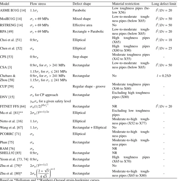
Table 4: Burst model summary properties

Model Flow stress Defect shape Material restriction Long defect limit

ASME B31G [14] 1.1 y Parabolic Low toughness pipes (be-_{low X56)} l2/D t = 20

ModB31G [14] y+69 MPa Mixed shape Low-to-moderate tough-_{ness pipes (below X65)} l2/D t = 50

RSTRENG [14] y+69 MPa Effective area No l2/D t = 50

RPA [49] y+69 MPa Rectangle + Parabolic Low-to-moderate tough-_{ness pipes (below X65)} l2/D t = 20

Choi et al. [51] 0.9 u Elliptical High_(X65) toughness pipes l2/D t = 18

Chen et al. [52] u Elliptical High_{(X80 to X90)}toughness pipes l2/D t = 25

CPS [53] 0.9 u Step shape Moderate toughness pipes_{(X42 to X55)}

-CSA [3] 0.9 ufor y>241 MPa Rectangular

Low-to-moderate

tough-ness pipes (below X65) l2/D t = 50 1.15 yfor y 241 MPa

Chebaro &

Zhou [58] 0.9 ufor y

>241 MPa Rectangular No l = 0.25D

1.15 yfor y 241 MPa

CUP [59] u Regular shape - groove Moderate toughness pipes_{(X46 to X60)}

-DNV [15] ufor CP approach Rectangular Excluding high toughnesspipes (X80)

-m ufor a given safety level

FITNET FFS [64] u(1/2)65 y1 Rectangular NR l2/D t = 20

Ma et al. [81]** 2 u/3(n+1)/2n Elliptical Excluding low toughness_pipes

-Netto et al. [16] 1.1 y Elliptical Moderate-to-high tough-_{ness pipes (X52 to X77)}

-Wang et al. [67] 1.1 y Rectangular + Elliptical No

-PCORRC [71] u Elliptical Moderate-to-high tough-_{ness pipes}

-Phan [75] u Rectangular Moderate-to-high tough-_{ness pipes}

-RAM [76] u NR

-SHELL92 [85] 0.9 u Rectangular NR

-Yeom et al. [73, 74] 0.9 u Rectangular High_{(X65 to X70)}toughness pipes

-Zhu et al. [79]* 2 u/3(n+1)/2 Rectangular No

-Zhu et al. [80]* 2 u

0 BBBB@2 +p3

4p3 1

CCCCAn+1 Rectangular Moderate-to-high tough-_{ness pipes (X65 to X80)} -Based on *Holloman and **Ramberg-Osgood strain-hardening curves.

This table shows that elliptical defect shapes were preferred for approaches using FEM simulations (e.g., Choi, Chen, Netto, Wang, PCORRC, and Ma), whereas those from codes like ASME, CSA, and DNV commonly proposed rectangular defect shapes for an additional level of conservatism in pipeline assessment. Regarding the flow stress, which is associated with the corresponding plastic collapse of the pipe, it lies within the yield and ultimate strengths except for the models that include the strain-hardening coefficients because they approximate the true strain-stress curve of the steel. This table also indicates that the reviewed models are appropriate for a certain material toughness:

• Low toughness pipes (Below X55): ASME B31G, ModB31G, RPA, CPS, CSA, CUP, DNV, Netto RAM, and SHELL;

• Moderate toughness (X55 to X65): ModB31G, RPA, Choi, CSA, CUP, DNV, Ma, Netto, Wang, PCORRC, Phan, Yeom, and Zhu; and

• High toughness (above X65): Chen, Ma, Netto, PCORRC, Phan, Yeom, Zhu.

There are some models with not announced restrictions in the public literature like Fitnet FFS, RAM, and SHELL that can be used in principle for any pipeline bearing in mind this limitation.

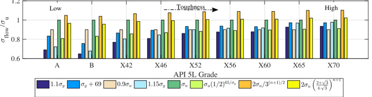
Material restrictions should be considered because inappropriate model selection may produce exaggerated conser-vative results. An arbitrary selection inherently assumes that the prediction capabilities of a model remain unchanged although the model was calibrated with specific burst tests. To properly compare the models level of conservatism, the ratio of the flow-to-ultimate strength was determined for each material reported by the API 5L and depicted in Fig. 6. According to Benjamin, an approach with a smaller ratio would be more conservative [42]. Note that the ASME B31G, Netto and Wang approaches (1.1 y) decrease their level of conservatism with the steel toughness obtaining

flow stresses close to the reported ultimate strength. Considering that approaches from Netto and Wang were designed for moderate-to-high toughness pipes, this result suggests that both approaches are more suitable than standards like ASME and CSA, as it was previously pointed out by Hasan et al. [20] and Teixeira et al. [45]. Note also that the mod-ifications of ASME (i.e., ModB31G, RSTRENG, and RPA) were proposed to decrease the level of conservatism in low toughness pipelines, which is the range of applicability of this model. Finally, Fitnet FFS approach ( u(1/2)65 y1)

could be too protective with a failure threshold lower than ASME for moderate-to-high toughness pipelines, which prevents it to be selected in these cases.

A B X42 X46 X52 X56 X60 X65 X70 API 5L Grade 0.6 0.8 1 1.2 σ flow / σ u 1.1σy σ_y+ 69 0.9σ_u 1.15σ_y σ_u σ_u(1/2)65/σy _2σ u/3(n+1)/2 2σu !_2+√3 4·√3 "n+1 High Low Toughness

Figure 6: Flow-to-ultimate stress ratio comparison

4.2. Metal loss acceptability

The failure criteria described through the flow stress is restricted to intact pipelines. Defect information like the shape idealization or its dimensions is not considered yet. To evaluate these parameters in the comparison, the acceptable depth to withstand the pipe maximum operating pressure (MAOP) was determined for each approach given a defect length. The latter considering that these parameters affect appreciably the burst pressure [51], particularly the defect depth in models like Netto and ASME B31G [45]. For this purpose, three case studies are proposed for a low, moderate and high toughness pipelines considering the toughness restrictions of each model, and a MAOP with the 72% of allowable stress. The properties of each case are presented in Table 5, whereas Figure 7 depicts the acceptable diagram using dimensionless variables d/t and l2_{/D t in which the burst pressure would rise up to the}

operating pressure for low (Figure 7a-b), moderate (Figure 7c-d), and high (Figure 7e-f) toughness pipes.

A defect is acceptable according to a burst model if its defect depth is lower than the reported in Fig. 7 given a specific l2_{/D t. Note these figures also include long defects like in the case of ASME B31G, where exaggerated}

con-servative results are obtained by requiring defects depth be lower than 0.4 t to prevent a burst (Fig. 7b). These figures also show that RAM approach can be considered as a lower boundary of acceptable defects due to its independence with defect length.

Table 5: Case studies for acceptable diagrams. Parameter _toughnessLow _ToughnessModerate _ToughnessHigh

D [mm] 304.8 610 1016 t [mm] 6.35 7.1 18.4 y[MPa] 320 450 552 u[MPa] 435 535 650 E [MPa] 207000 207000 206000 MAOP [MPa] 9.6 7.54 14.39 Pipe material X46 X65 X80 0 5 10 15 20 l2/Dt 0.4 0.6 0.8 d/t a) 20 25 30 35 40 45 50 l2/Dt 0.3 0.4 0.5 0.6 d/t b) 0 5 10 15 20 l2/Dt 0.4 0.6 0.8 d/t c) 20 25 30 35 40 45 50 l2/Dt 0.3 0.4 0.5 0.6 d/t d) 0 5 10 15 20 l2/Dt 0.4 0.6 0.8 d/t e) 20 25 30 35 40 45 50 l2/Dt 0.3 0.4 0.5 0.6 d/t f) ASME B31G Chen Choi CPS CSA Z662-07 CUP DNVRP-F101 FITNET FFS Ma ModB31G NETTO PCORRC Phan 1 Phan 2 Phan 3 RAM RPA SHELL92 Wang Yeom Zhu(2004) Zhu(2015)

Figure 7: Acceptable diagram for: a) low, b) low (continued), c) moderate, d) moderate (continued), e) high, and f) high (continued) toughness

In regard of the three case studies, the results show that the RPA approach increments the level of conservatism of ModB31G for long defects in low-to-moderate toughness pipes almost until the prediction of RAM, whereas the ap-proaches of Choi and Chen presents less noticeable changes for moderate and high toughness pipelines, respectively. These figures also indicate some common performances among the models reviewed. For low toughness pipes, there are three clear approaches with similar behaviors: i) CPS, DNV, and ModB31G; ii) CSA, Fitnet, and SHELL; and iii) the approach of CUP that lies between them. Figure 7a also shows that the CUP approach is overly conservative for almost impact pipelines with an acceptable depth lower than 0.6 t to prevent a burst. These results indicate that approaches like ASME B31G, RAM, and CUP would overestimate the real strength of the pipeline and unneces-sary intervention can be implemented. However, the CUP model could be an interesting approach for long defects with l2_{/D t > 20. For moderate toughness pipes, Figure 7c-d suggest two model clusters: i) ModB31G, DNV, Ma,}

PCORRC, and Zhu; ii) CSA, Phan(1-2), SHELL, Yeom, and Wang. Two additional models lie between these clusters, i.e., Phan (1) and Choi, and finally, the model of Netto that is not conservative at all, except for short defects with the approach of Zhu. These results indicate that approaches like DNV, Ma, PCORRC, and Zhu are interesting models to be considered for pipes with a moderate toughness. Finally, Figure 7e-f present the results for high toughness pipes exposing two model clusters: i) Chen, PCORRC, Ma, and Zhu; ii) Phan and SHELL, which again confirms that the

same approaches as for moderate toughness pipes including the model of Chen.

Similar results were determined by other comparisons based on calculated failure probabilities. Hasan et al. [20] compared the standards ASME B31G, DNV RP F-101 (the capacity -CP- and the maximum allowable pressure -MOP-approaches), CSA Z662-07, and the approach of Netto et al. [16] using Monte Carlo simulations and First Order Second Moment (FOSM) methods. Their results indicate that the DNV (MOP) and CSA approaches are conservative in comparison to ASME B31G, Netto, and DNV (CP). Additionally, they concluded that the standard DNV RP F-101 (CP) is adequate for moderate to high toughness pipelines, whereas the ASME B31G approach could be applicable for any toughness steel based on sensitivity analysis of the failure probability and burst pressure. They recommended the DNV approach for new hardened pipes and ASME B31G or CSA Z662 for both new and old pipes because of their closeness with the results obtained with the model of Netto and co-workers. Another interesting comparison was developed by Caleyo et al. [88] using the ASME B31G, Modified B31G, PCORRC, DNV RP –A version launched in 1999 without the factor 1.05 in Eq. 30–, and SHELL92 approaches. They evaluated several influences on the failure probability and the rate of repairs of a pipeline: the methods to calculate the failure probability, the resistance/load variables distribution, and these coefficients of variation of these distributions. The results of Caleyo et al. [88] showed that the SHELL92 and ASME B31G approaches, respectively, obtained the highest and lowest failure probabilities, which could be attributed to the significance of the defect depth, length, and the operating pressure for the ASME B31G approach [88]. Furthermore, they concluded that defects which depths are around 15% of the wall thickness depend significantly on the burst model, whereas depths about 50% of the wall thickness this dependence is highly undetected. In this case, it can be said that the difference in burst predictions are almost infinitesimal for longer defects.

4.3. Failure probability comparison

To evaluate now the sensitivity of each approach with the defect depth, the failure probability of the reviewed models were determined by implementing the case study reported in Hasan et al. [20]; i.e. an API 5L X65 pipeline with the properties shown in Table 6, which is subject of a degradation process predicted by the SwRI model [89].

Table 6: Case Study reported by Hasan et al. [20].

Parameter u[MPa] y[MPa] D [mm] t [mm] P [MPa] l [mm]

Mean 531 448 713 20.24 17.12 340

COV 0.05 0.07 0.001 0.001 0.08 0.5

Distribution Lognormal Lognormal Normal* Normal* Gumbel Weibull *Truncated at 0.

The failure probability was then calculated with Monte Carlo simulations using an operating pressure based on the yield pressure (for a defect-free pipe) and a safety factor of 72%. The obtained results are depicted in Fig 8,where the model of RAM using Eq. 42 is also included. This figure shows similar performances regarding a certain failure (Pf ⇡ 1 about t=30 years) with a relatively different evolution for the CSA Z662 approach. Besides, the results

indicate that RAM, SHELL92, Fitnet FFS, Wang’s model and CSA Z662 (after 10 years) may obtain conservative burst failure predictions in comparison with the other approaches. Note that a failure probability of 0.5 for these approaches is reached from 8 (RAM) to 12 (SHELL) years, which is lower than the 17 years predicted by the Model of Netto. The early failure of CSA was unexpected considering the results of Zhou & Huang [19]; however, a similar pattern was obtained using information from In-Line inspection [90]. This result may be attributed to the conservatism of moderate-to-high toughness pipelines mentioned by Hasan et al. [20]. Specifically for the RAM predictions, the conservative results are linked with the use of minimum wall thickness instead of the nominal wall thickness as the other burst pressure models. The failure probability of RAM-Med is clearly less conservative based on the reliability in comparison to the other approaches.

Regarding the burst pressure, Table 7 depicts the results for the mean and coefficient of variation (COV) of each model. The majority of the evaluated models follow a common pattern starting near 30 MPa for intact pipelines and reaching a final burst pressure about 16 MPa, after 15 years of corrosion degradation. Bearing in mind that DNV is one of the more accurate burst models for defect-free pipes, the results shown in Table 7 for the first evaluating year, reveal that approaches like Chen, CPS, Ma, RAM, and Zhu may also have good predictions. However, the models of RAM and Chen are more sensitive to depth metal loss by obtaining a difference of 11 MPa between RAM and DNV

0 5 10 15 20 25 30 Time (years) 0 0.1 0.2 0.3 0.4 0.5 0.6 0.7 0.8 0.9 1 Failure probability ASME B31G Chen Choi CPS CSA Z662-07 CUP DNVRP-F101 FITNET FFS Ma ModB31G NETTO PCORRC Phan 1 Phan 2 Phan 3 RAM RAM-Med RPA SHELL92 Wang Yeom Zhu(2004) Zhu(2015) Figure 8: Failure Probability comparison for the selected models

after 15 years of evaluation, so their predictions may be too conservative for pipelines with deeper defects. Indeed, the COV presented in Table 7 shows that Netto and RAM have the lowest and highest COV for burst predictions, respectively, which confirms the above statement. The COV propagation rates were almost constant for DNV, FFS, Phan(2), Yeom, SHELL, Zhu (2004), and PCORRC; increasing for CSA, Choi, and CPS; and decreasing for ASME B31G, Chen, CUP, Ma, ModB31G, Phan(1-3), RAM, RPA, Wang, and Zhu(2015). In addition, the propagation results of the models Phan were close to the structure they were developed, i.e., Netto (Phan 1), FFS (Phan 2), and PCORRC (Phan 3), which was expected. The aforementioned results would suggest that models with decreasing or stable propagation rates are suitable for the predictions of the burst pressure. In case of a moderate toughness pipe like the case study, models like DNV, Ma, Netto, PCORRC, and Zhu can be suggested in advance.

Table 7: Mean and COV results of the predicted burst pressure

Parameter Mean Pb COV Pb

Year 1 5 10 15 1 5 10 15 ASMEB31G 27.50 25.44 22.80 20.42 0.03 0.08 0.13 0.18 Chen 33.58 28.75 23.24 18.97 0.04 0.10 0.17 0.22 Choi 24.75 23.71 21.17 18.12 0.10 0.07 0.13 0.20 CPS 33.77 29.73 24.23 19.06 0.04 0.09 0.18 0.26 CSA 26.81 24.11 19.97 14.58 0.03 0.06 0.12 0.24 CUP 29.44 26.42 22.45 18.86 0.03 0.08 0.14 0.19 DNV 32.02 29.42 25.48 21.37 0.03 0.08 0.16 0.24 FFS 27.39 24.42 20.21 16.13 0.03 0.10 0.18 0.27 Ma 32.18 28.21 23.66 20.16 0.03 0.09 0.15 0.19 ModB31G 28.80 26.40 23.07 19.90 0.03 0.07 0.13 0.18 Netto 27.81 26.25 23.23 20.08 0.02 0.06 0.11 0.15 PCORRC 29.60 27.18 23.72 20.24 0.02 0.08 0.14 0.21 Phan 1 27.14 23.88 20.08 17.04 0.03 0.09 0.13 0.16 Phan 2 27.36 24.67 21.03 17.60 0.03 0.10 0.18 0.26 Phan 3 27.22 24.15 20.53 17.59 0.03 0.09 0.15 0.20 RAM 30.04 22.12 15.19 10.34 0.08 0.16 0.25 0.30 RPA 28.78 26.26 22.83 19.58 0.03 0.08 0.15 0.21 SHELL 26.48 23.61 19.54 15.60 0.03 0.10 0.18 0.27 Wang 27.30 23.86 19.19 15.16 0.03 0.10 0.18 0.23 Yeom 26.51 23.81 20.05 16.41 0.03 0.09 0.17 0.25 Zhu (2004) 32.39 29.74 25.96 22.15 0.02 0.08 0.14 0.21 Zhu (2015) 30.10 27.43 24.27 21.71 0.03 0.08 0.14 0.19