HAL Id: hal-01231807
https://hal.inria.fr/hal-01231807
Submitted on 20 Nov 2015
HAL is a multi-disciplinary open access
archive for the deposit and dissemination of
sci-entific research documents, whether they are
pub-lished or not. The documents may come from
teaching and research institutions in France or
abroad, or from public or private research centers.
L’archive ouverte pluridisciplinaire HAL, est
destinée au dépôt et à la diffusion de documents
scientifiques de niveau recherche, publiés ou non,
émanant des établissements d’enseignement et de
recherche français ou étrangers, des laboratoires
publics ou privés.
Florent Loete, Qinghua Zhang, Michel Sorine
To cite this version:
Florent Loete, Qinghua Zhang, Michel Sorine.
Experimental validation of the inverse
scat-tering method for distributed characteristic impedance estimation.
IEEE Transactions on
An-tennas and Propagation, Institute of Electrical and Electronics Engineers, 2015, 63 (6), pp.7.
�10.1109/TAP.2015.2417215�. �hal-01231807�
Abstract— Recently published theoretic results and numerical
simulations have shown the ability of inverse scattering-based methods to diagnose soft faults in electric cables, in particular, faults implying smooth spatial variations of cable characteristic parameters. The purpose of the present paper is to report laboratory experiments confirming the ability of the inverse scattering method for retrieving spatially distributed characteristic impedance from reflectometry measurements. Various smooth or stepped spatial variations of characteristic impedance profiles are tested. The tested electric cables are CAN unshielded twisted pairs used in trucks and coaxial cables.
Index Terms—Inverse scattering, cable health monitoring, soft
fault diagnosis, frequency domain reflectometry.
I. INTRODUCTION
HE FAST development of electronic devices in modern engineering systems comes with more and more connections through cables, and consequently, the reliability of electric connections becomes a crucial issue. For example, in a modern automotive vehicle, the total length of onboard cables has tremendously increased during the last decades and is now up to 4km. These cables are composed of twisted pairs, coaxial cables, simple wires and many different connectors. These wires and connectors are subject to aging or degradation because of severe environmental conditions. In this area, reliability becomes a safety issue. In some other domains, cable defects may have catastrophic consequences [1]. It is thus a crucial challenge to design smart embedded diagnosis systems able to detect wired connection defects in real time. This fact has motivated research projects on methods for fault diagnosis in electric transmission lines.
Many diagnosis methods based on Time or Frequency Domain Reflectometry (TDR or FDR) have been developed to detect, locate and characterize defects in electrical harnesses [2]-[9][5]. These methods are based on the same principle as radar technology, but applied to guided waves in electric cables. A high frequency electrical signal is sent down a cable, where it
1 Florent Loete is with GEEPS-SUPELEC, 11 rue Joliot Curie 91192 Gif sur Yvette, France. Contacting author email : florent.loete@supelec.fr
2 Qinghua Zhang is with Inria Rennes, Campus de Beaulieu, 35042 Rennes, France.
is reflected at impedance discontinuities or at other inhomogeneities along the cable. The reflected wave is analyzed to detect, locate and characterize the defects. It has been reported that this technology is able to detect and to locate hard faults (open or short circuits) up to an accuracy of about 3 cm [6]. On the other hand, it is a much more difficult problem to deal with soft faults which imply only smooth and localized characteristic impedance changes in electric cables. Some recent methods have been reported that amplify fault signatures and improve the detection of the small echoes caused by soft faults [10]-[15] but, except for connectors [9], to our knowledge, no satisfactory experimental result of reflectometry-based method for the diagnosis of such soft faults has been reported.
The characteristic impedance is the main parameter characterizing an electric cable. When a healthy and uniform cable is considered, the characteristic impedance is usually specified as a single value for the whole cable. In order to deal with localized defects, it is necessary to consider distributed characteristic impedance all along the cable, denoted as with indicating the position along the cable in some coordinate system.
In traditional reflectometry-based methods, the reflected waveforms are visualized and analyzed in the time domain (TDR) or in the frequency domain (FDR), and sometimes a mixture of them is used. As these methods do not directly analyze the characteristic impedance of the cable, it may be difficult to interpret their results for soft faults diagnosis, in particular when such faults do not cause any discontinuity, but only smooth4 variations of the characteristic impedance along the cable. It is thus useful to develop inverse methods retrieving the spatially distributed characteristic impedance profile from reflectometry measurements (in opposition to direct methods simulating reflectometry measurements from specified cable characteristics), but few methods of this nature have been reported [16]. The inverse scattering theory [17] provides a powerful theoretic framework for the estimation of distributed characteristic impedance from reflectometry measurements, in particular for smoothly varying characteristic impedance profiles along cables. Based on this theory, the ability of
3 Michel Sorine is with Inria Paris-Rocquencourt, Domaine de Voluceau, 78153 Le Chesnay, France.
4 The meaning of "smoothness" will be specified in Section II.
Experimental validation of the inverse scattering
method for distributed characteristic impedance
estimation
Florent Loete
(1),
Qinghua Zhang
(2), and
Michel Sorine
(3)interpretation and processing of reflectometry measurements, notably for the purpose of soft fault diagnosis.
The theoretic study and numerical simulations reported in [18],[19] have shown that the inverse scattering method is a promising tool for soft fault diagnosis through the estimation of distributed characteristic impedance. The purpose of the present paper is to confirm these results through laboratory experiments. Some preliminary experiments have been presented in [20]. The present paper presents more complete experimental results, including a study on the errors of characteristic impedance estimation by the inverse scattering method.
This paper is organized as follows. After briefly recalling in Section II the inverse scattering method for electric cable monitoring, in Section III experimental results will be presented with cables exhibiting smooth characteristic impedance variations. The robustness of the inverse scattering method to characteristic impedance discontinuities is experimentally studied in Section IV. Section V then concludes the paper.
II. THE INVERSE SCATTERING METHOD
This section shortly recalls the inverse scattering method for lossless cables. More details can be found in [18]. For the electric cables of less than 10 meters length studied in this paper, losses are neglected. A lossless cable driven by a harmonic voltage wave can be modeled by the frequency domain telegrapher's equations
, , 0 (1a)
, , 0 (1b)
where is the angular frequency (denoted so because it is strongly related to the wavenumber in the inverse scattering theory), , and , denote the voltage and the current, and are distributed inductance and capacitance at the point along the cable; is the imaginary unit. The boundary conditions associated to (1) represent a generator at the left end and a load at the right end of the cable.
Define the electrical distance, the characteristic impedance, the reflected and direct power waves, as follows5
, ∈ 0,
(2)
ν , , , (3a)
5 Where is the length of the cable and is a monotonic function, implying the existence of its inverse function . By abuse of notation,
Some direct computations then lead to the following
Zakharov-Shabat equations [17]: ν , ν , ν , (4a) ν , ν , ν , (4b) where (5)
In theory, it is assumed that the function is absolutely continuous, so that its scattering transform is well defined [21]. This smoothness assumption means essentially that is continuously differentiable and does not vanish on the interval 0, . In practice it excludes high frequency variations beyond the instrumentation bandwidth.
At the left end (corresponding to 0), the reflection coefficient ν , 0 /ν , 0 is typically measured with a network analyzer. It is known [18] that the characteristic impedance can be computed from measured at the left end of the cable through the following steps:
1. Compute the Fourier transform of the reflection coefficient .
21 exp
2. Solve the integral equations (known as Gel'fand-Levitan-Marchenko equations) for their unknown kernels
, and , :
, , 0
, , 0
3. Compute the potential function through:
2 ,
4. By solving equation (5) for , compute:
0 2
where 0 is equal to the internal impedance of the signal generator connected to the left end of the cable (typically integrated in a network analyzer).
V , will be simply written as V , , so will other similar notations depending on .
III. EXPERIMENTS WITH TWISTED PAIRS
In order to experimentally validate the inverse scattering method for estimating the distributed characteristic impedance along a cable, we need to configure electrical cables with known smooth spatial variations of the characteristic impedance. It is realized with twisted pairs for the experiments reported in this section.
A. Inverse scattering for a cable with smoothly varying impedance profile
The characteristic impedance profile of a cable composed of two wires can be easily modified by controlling locally the distance between the two wires. Based on a geometrical model of the cable characteristics, particular forms of the characteristic impedance profile can be realized in this way. Such modified cables will be used to experiment the inverse scattering method, by comparing the characteristic impedance profile computed by inverse scattering method with the one known from the geometric model.
In the lossless case, the characteristic impedance , as defined in equations (2), depends only on the inductance L and the capacitance C per unit length. It is known that L and C for a cable composed of two wires are determined by the radius r of the copper wires, the distance D between the two wires, the magnetic permeability and the dielectric permittivity of the air and the relative dielectric permittivity of the dielectric insulation, as formulated in the following equations:
(6a)
(6b) By choosing the distance between the two wires as a
function of z, a particular characteristic impedance profile can be obtained. In this study, a cosine function is chosen:
1 2 (7)
where 2mm is the diameter of the insulated wire, A = 4mm and l = 25cm, as shown in Fig 1. Following (6a), (6b) and (7) the computed distributed characteristic impedance corresponding to the cosine profile D(z) is shown in Fig. 2
Fig. 1: Untwisted pair with a cosine profile .
Fig. 2: Distributed characteristic impedance corresponding to the cosine profile.
Before applying the inverse scattering method to such a cable, let us first experimentally verify the model of based on (2), (6a) and (6b). Given the characteristic impedance profile computed through (2), (6a), (6b) and (7) as shown in Fig. 2, we numerically simulate the impulse response (also known as the reflectogram) of the cable, and compare this simulated impulse response with the experimentally measured impulse response of the true cable. The experimental setup is presented in Fig. 3. At the left end, the cable is connected to a network analyzer (VNA), and the right end the cable is terminated by a 110 Ω resistance as load. The reflection coefficient measurement is carried out over the 2 MHz - 1.102 GHz with 2 MHz frequency steps. The impulse response of the line is then obtained by computing the IFFT of the reflection coefficient. The results presented in Fig. 4 show a satisfactory agreement between the simulated and the experimental impulse responses of the tested cable. The maximum error is about 25% of the magnitude of the impulse response.
Now we are going to apply the inverse scattering method to the same cable in order to retrieve the distributed characteristic impedance profile from the reflection coefficient measured with the network analyzer. Fig. 5 shows the results of the inverse scattering method for two experiments made on the same cable but with two different loads connected at the right end (resistances of 110 Ω and 220 Ω). The two curves in Fig. 5 are almost identical except at their right ends. The highest bump corresponds to the part of untwisted wires shown in Fig. 1. The right ends of the two curves correspond to the loads of 110 Ω and 220 Ω connected in the two experiments. The fact that the two curves are almost identical in their major part suggests that the variations in the two curves, except at the right end, do correspond to the geometrical variations of the same tested cable.
In Fig. 6 the part corresponding to the cosine untwisted wires is zoomed and compared to the curve computed from (2), (6a), (6b) and (7). The maximum error in percentage of the estimated characteristic impedance is similar to that of the impulse response shown in Fig. 4. The errors can be partly explained by the fact that the losses in the cable are neglected by the inverse scattering method. This fact is further confirmed by two more experiments with a longer cable segment inserted between the network analyzer and the cosine untwisted wires. As shown in Fig. 7, the part corresponding to the cosine untwisted wires (the same as in the previous experiments) produces a lower bump of
untwisted part of the wires from the network analyzer, the more important is the effect of the losses neglected by the inverse scattering method. Nevertheless, if this artificially made characteristic impedance variation was caused by a fault of the cable (smooth variation of about 170 Ω), the accuracy of the inverse scattering method would be sufficient enough for the detection, location and characterization of the fault.
Fig. 3: Experimental setup. The cosine profile is inserted between two 110Ω twisted pair segments.
Fig. 4: Simulated (-) and experimental (- -) impulse responses of the cable illustrated in Fig. 3.
Fig. 5: Inverse scattering performed on the cable including the cosine profile in two experiments, one with a 110 Ω load (-) and the other with a 220 Ω load (-
-).
Fig. 6: Comparison of the measured (-) and simulated (- -) characteristic impedance of the cosine part of the cable.
In Fig. 7 the right ends of the two lines correspond to the two loads connected to the right end of the cable in the two experiments. There is a 14% error on the estimation of the 220 Ω. One explanation of this error is the effect of the losses neglected by the inverse scattering method. Another source of error is the impedance mismatch between the cable and the load, implying an impedance discontinuity, a case that is not covered by the inverse scattering method, in theory. More discussions about impedance discontinuities will be made in Section IV.
Fig. 7:Inversescattering performed on a longer twisted pair. The 0.25 m cosine profile is inserted between the two twisted pair segments of respectively 5.9 m and 0.9 m. In the two presented experiments the line is terminated with a 110 Ω load (-) or with a 220 Ω load (- -).
B. Application to the monitoring of connectors on an automotive electrical harness
The characteristic impedance variation studied in the previous experiments is similar to those observed around connectors in automotive harnesses (see Fig. 8) where the distance between the two wires is increased. We then applied the inverse scattering method to the monitoring of twisted pairs and their connectors used in a truck. A cable of 5.4m long is linked to 0.9m of similar cable through the connector shown in Fig. 8. As shown in Fig. 9, the connector's location and the impedance variation caused by the connector can be inspected by the inverse scattering method. It is then possible to elaborate some
diagnosis rules of the connector based on the evolution of the estimated impedance profile over the time [9].
Fig. 8:Spatial spacing variation of the two wires of a twisted pair around an automotive connector.
Fig. 9: Monitoring of a connector's impedance profile with the inverse scattering method.
IV. ROBUSTNESS OF THE INVERSE SCATTERING METHOD TO IMPEDANCE DISCONTINUITIES
Since equation (4) contains the spatial derivative of the characteristic impedance, it is assumed in theory that is derivable. Consequently, the inverse scattering method presented in section II is, in theory, limited to smooth characteristic impedance profiles, thus excluding the case of impedance discontinuities. Impedance discontinuities are frequently present in practice, typically at the connection between the network analyzer and the tested cable if there is an impedance mismatch. Nevertheless, experimental results reported in the previous section show that the inverse scattering method can tolerate impedance discontinuities to some extent, as e.g. with the impedance mismatch between the network analyzer and the cable, or with the mismatched load. The aim of this section is to further study the robustness of the inverse scattering method in presence of impedance discontinuities and to quantify the error.
The experiments presented in this section are designed with 50 Ω coaxial RG-58 cables with low loss characteristics. They also have good noise immunity, and a well-controlled spatially homogeneous 50 Ω characteristic impedance. The tested configurations are very simple, but they are in no way favorable to the inverse scattering method, because of impedance discontinuities. The accuracy of the characteristic impedance of
the coaxial cables allows us to quantitatively evaluate the error of the inverse scattering method. The measurements are carried out over the 4 MHz – 2204 MHz bandwidth with 4 MHz frequency steps.
In this section, coaxial cables will be used to build composite lines with piecewise constant characteristic impedance profiles. However, the applied inverse scattering algorithm is exactly the same one as in the previous section, which does not assume piecewise constant characteristic impedance profiles.
A. Characteristic impedance drop on a single segment
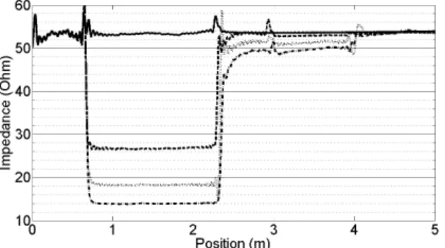
Two identical 50 Ω coaxial cables in parallel (Fig. 10) are used as an equivalent cable of 25 Ω. Similarly, three and four identical cables in parallel form respectively equivalent 16.67 Ω and 12.5 Ω cables. Such a composite segment is then connected to simple 50 Ω coaxial cables as shown in Fig 10 and illustrated in Fig. 11, in order to build a cable with piecewise constant characteristic impedance. The advantage of this configuration is the accuracy of the characteristic impedance (50 Ω, 25 Ω, etc.) in each segment, based on the high quality coaxial cables used in the experiment.
.
Fig. 10: Composite line including two RG-58 50 Ω coaxial cables in parallel.
Fig. 11: Topology of the composite lines used. Equivalent cables of characteristic impedance smaller than 50 Ω are realized by putting multiple 50Ω coaxial cables in parallel.
Fig. 12 shows the inverse scattering results carried out on the cables illustrated in Fig. 11. The location of impedance discontinuities, as well as the impedance level of the composite segment, are estimated with a good accuracy. Nonetheless, one can see some artifacts in the part immediately following the segment composed of parallel cables, especially for strong impedance discontinuities. It is possible to remedy this drawback by increasing the bandwidth of the reflectometry measurements, but in practice the network analyzer has a limited bandwidth. These artifacts are also reduced by adding zeros to complete high frequency measurements (zero padding), because the inverse scattering algorithm then uses a smaller integration step size. For example, in one of the experiments, the same reflection coefficient is processed twice by the inverse scattering method, first with zero padding up to
However, the practice of zero padding is limited by the computer memory size when the data are processed. The results shown in Fig. 12 have been obtained with zero padding up to 30 GHz.
Remember that this study is only for the purpose of evaluating the robustness of the inverse scattering method to impedance discontinuities. If it is known in advance that the tested cable has a piecewise constant characteristic impedance profile, some other methods designed for this particular case may be more appropriate.
Fig. 12: (z) profiles obtained by inverse scattering on the line including an (equivalent) segment of (-) 50 Ω (- -) 25 Ω (▪▪) 16.6 Ω and (▪ ─) 12.5 Ω.
Fig. 13: Comparison of two Z (z) profiles obtained by inverse scattering on the same line including an (equivalent) segment of 12.5 Ω with zero padding up to 15 GHz (-) and 30 GHz (--). These results show that a higher zero padding leads to a more accurate result.
B. Double characteristic impedance drop
This example is intended to study the ability of the inverse scattering method to estimate more complex discontinuous characteristic impedance profiles.
Fig. 14: Above: Two segments of doubled and tripled cables inserted in the middle of a 50 Ω coaxial. Below: Result of the inverse scattering method.
As shown in Fig. 14, in the middle of a 50 Ω coaxial cable, a segment of doubled cables and another one of tripled cables are inserted, with equivalent characteristic impedances of 25 Ω and 16.67 Ω. The result of the inverse scattering method is also shown in Fig. 14. The characteristic impedance profile is estimated with a good accuracy, despite the multiple discontinuities present in the characteristic impedance profile. In Fig. 14, the estimated characteristic impedance profile exhibits spikes at each junction between the different segments of the line (e.g. at the injection point, at the connection of the 50 Ω coaxial cable and the segment of doubled cables etc). These are caused by the 50 Ω connectors which are slightly improperly adapted to the line and furthermore locally add some extra lengths to the line (each straight or Tee connector adds about 2cm to the 50 Ω coaxial line). This explains the small two first impedance spikes observed at 0m and 0.6m. The spike at the third connection point (between the 25 Ω and the 16.66 Ω segments) is all the more observed since 3 BNC Tees are stacked in order to connect the doubled and tripled cables segments.
C. Accuracy of the inverse scattering method in the case of piecewise constant characteristic impedance profiles.
Remember that, in theory, the case of characteristic impedance with discontinuities is not suitable for the inverse scattering method. Nevertheless, the reported experiments show that this method can tolerate discontinuities to some extent. The results of section IV.A show that, the higher is the step jump of the characteristic impedance, the larger is the error of the inverse scattering method. To complete these results, numerical simulations have been made to further characterize the errors. The simulated cable configurations are similar to that of Fig. 11, but the characteristic impedance level jump in the
middle segment can be freely chosen for numerical simulations. The reflection coefficients of the simulated cables with various impedance level jumps ΔZ are simulated in the
50Ω; 350Ω range and then are given as input to the inverse scattering method. The relative accuracy of the inverse scattering method was calculated as:
% ∆ ∆
∆
where ∆ is the impedance level jump of the middle segment estimated by the inverse scattering method. The results are plotted in Fig. 15. As expected, the error is increasing with ΔZ. Therefore, in presence of strong impedance jumps, the error term can rapidly reach quite high values. Nevertheless, when ∆ ∈ 50Ω; 100Ω , the error is less than 5%. So one must be careful when interpreting impedance values computed in presence of strong discontinuities.
When both smooth variations and discontinuities are present in the characteristic impedance profile of a cable, the reflection coefficient measured at one end of the cable is the result of all these imperfections of the cable. As waves injected in a cable are essentially reflected at the discontinuities, too strong discontinuities may mask the effects of the reflections caused by smooth variations. It is thus important to avoid strong discontinuities when smooth variations should be monitored. In the experiments reported in the previous section, it was shown that an impedance jump of 60 Ω (impedance mismatch between the network analyzer and the 110 Ω cable), and another one of 110 Ω (impedance mismatch between the 110 Ω cable and the 220 Ω load) are well tolerated when smoothly varying characteristic impedance profiles are estimated, with a satisfactory accuracy for the purpose of soft fault detection, location and characterization.
Fig. 15: Inverse scattering method accuracy in case of impedance discontinuities. (▲)Accuracy obtained from the inversion of experimentally measured reflection coefficient. (■) Accuracy obtained from the inversion of simulated reflection coefficient.
V. CONCLUSION
The experimental results presented in this paper confirm the previously reported theoretic results and numerical simulations about the inverse scattering method. These results provide a new way for the interpretation of reflectometry measurements. In the first experiment, a spatially smooth variation of the characteristic impedance was created by modifying the spacing of the two wires of a twisted pair. This well-controlled profile
leads to a smoothly varying characteristic impedance, which can be computed through a geometric model of the cable. This result was in good agreement with the characteristic impedance profile estimated by the inverse scattering method. To further characterize the errors of the inverse scattering method, high quality coaxial cables were then used to build composite lines with piecewise constant characteristic impedance profiles. It is shown that the inverse scattering method can tolerate to some extent impedance discontinuities. The robustness of the inverse scattering method to moderate noises has been studied by numerical simulation in [18] where it is shown that, when the signal-to-noise ratio is 24dB, the result of the proposed method is still satisfactory.
The reported results confirm the ability of the inverse scattering method for estimating smoothly varying characteristic impedance profiles, with a satisfactory accuracy for the purpose of soft fault diagnosis in electric cables. Moreover, the implemented inverse scattering algorithm is numerically efficient: for each of the experiments presented in this paper, the processing of the data by the inverse scattering algorithm takes less than a second on a typical notebook computer.
VI. ACKNOWLEGMENTS
This work has been supported by the ANR SODDA project. REFERENCES
[1] C. Furse, Y. C. Chung, C. Lo, and P. Pendayala, “A Critical Comparison of Reflectometry Methods for Location of Wiring Faults,” Journal of
Smart Structures and System, vol. 2, no.1, pp. 25-46, 2006.
[2] C. Furse, and P. Smith, “Spread spectrum sensors for critical fault location on live wire networks," Journal of Structural Control and Health
Monitoring, vol. 12, pp. 257-267, June 2005.
[3] A. Lelong, M. Olivas Carrion, V. Degardin, and M. Lienard, “On line wiring diagnosis by modified spread spectrum time domain reflectometry," PIERS Proceeding, 182-186, Cambridge, USA, July 2-6, 2008.
[4] M.K. Smail, L. Pichon, M. Olivas, F. Auzanneau, and M. Lambert, “Detection of Defects in Wiring Networks Using Time Domain Reflectometry,” IEEE Transactions on Magnetics, vol. 46, no. 8, pp. 2998–3001, July 2010.
[5] C. Furse, Y.C. Chung, and R. Dangol, “Frequency domain reflectometry for on board testing of aging aircraft wiring,” IEEE Trans. EMC, vol. 45, no. 2, 2003.
[6] P. Smith, C. Furse, and J. Gunther, “Fault location on aircraft wiring using spread spectrum time domain reflectometry," IEEE Sensors Journal, vol.5, no. 6, pp. 1469-1478, December 2005.
[7] C. Furse, and N. Kamdar, “An inexpensive distance measuring system for navigation of robotic vehicles," Microwave and Optical Technology
Letters, vol. 33, no. 2, April 2002.
[8] Y. C. Chung, C. Furse, and J. Pruitt, “Application of phase detection frequency domain reflectometry for locating faults in an F-18 flight control harness," IEEE Transactions Electromagnetic Compatibility, vol. 47, no. 2, May 2005.
Electrical Contacts, 1-4, September 2012.
[10] M. Franchet, N. Ravot, and O. Picon, “The use of the pseudo wigner ville transform for detecting soft defects in electric cables," IEEE/ASME
International Conference on Advanced Intelligent Mechatronics (AIM),
309-314, July 2011.
[11] M. Franchet, N. Ravot, and O. Picon, “On a useful tool to localize jacks in wiring network," PIERS Proceedings, 856-863, Kuala Lumpur, Malaysia, March 27-30, 2012.
[12] L. El Sahmarany, F. Auzanneau, and P. Bonnet, “Novel reflectometry method based on time reversal for cable aging characterization," 58th
IEEE Holm Conference on Electrical Contacts, 1-6, September 2012.
[13] L. El Sahmarany, F. Auzanneau, L. Berry, K. Kerroum, and P. Bonnet, “Time reversal for wiring diagnosis," IEEE Electronic letters, vol. 48, no. 21, pp. 1343-1344, October 2012.
[14] L. Abboud, A. Cozza, and L. Pichon, “A matched-pulse approach for soft-fault detection in complex wire networks," IEEE Transactions on
Instrumentation and Measurement, vol. 61, no. 6, pp. 1719-1732, 2012.
[15] L. Abboud, A. Cozza, and L. Pichon, “A non-iterative method for locating soft faults in complex wire networks," IEEE Transactions on Vehicular
Technology, vol. 62, no. 3, January 2013.
[16] M.K. Smail, T. Hacib, L. Pichon and F. Loete, “Detection and location of defects in wiring networks using Time Domain reflectometry and neural networks,” IEEE Transactions on Magnetics, vol. 47, no. 5, pp. 1502-1505, May 2011
[17] M. Jaulent, “The inverse scattering problem for LCRG transmission lines," Journal of Mathematical Physics, vol. 23, no. 12, pp. 2286-2290, December 1982.
[18] Q. Zhang, M. Sorine, and M. Admane, “Inverse scattering for soft fault diagnosis in electric transmission lines," IEEE Trans. on Antennas and
Propagation, vol. 59, no. 1, 141-148, 2011.
[19] H. Tang, and Q. Zhang, “An inverse scattering approach to soft fault diagnosis in lossy electric transmission lines," IEEE Trans. on Antennas
and Propagation, Vol. 59, No. 10, 3730-3737, 2011.
[20] F. Loete, Q. Zhang and M. Sorine, “Inverse scattering experiments for electrical cable soft fault diagnosis and connector location” PIERS
proceedings, Kuala Lumpur, Malaysia, March 2012.
[21] A.G. Ramm, “A new approach to the inverse scattering and spectral problems for the Sturm-Liouville equation,” Annal. Der Physik, vol. 7, no. 4, pp.321-338, 1998.