HAL Id: hal-02393146
https://hal-mines-paristech.archives-ouvertes.fr/hal-02393146
Submitted on 4 Dec 2019
HAL is a multi-disciplinary open access
archive for the deposit and dissemination of
sci-entific research documents, whether they are
pub-lished or not. The documents may come from
teaching and research institutions in France or
abroad, or from public or private research centers.
L’archive ouverte pluridisciplinaire HAL, est
destinée au dépôt et à la diffusion de documents
scientifiques de niveau recherche, publiés ou non,
émanant des établissements d’enseignement et de
recherche français ou étrangers, des laboratoires
publics ou privés.
Urban-scale energy simulation: A development of a
novel method for parsimonious modelling -The example
of solar shading model calculation
Enora Garreau, Thomas Berthou, Bruno Duplessis, Vincent Partenay,
Dominique Marchio
To cite this version:
Enora Garreau, Thomas Berthou, Bruno Duplessis, Vincent Partenay, Dominique Marchio.
Urban-scale energy simulation: A development of a novel method for parsimonious modelling -The example
of solar shading model calculation. BS2019, Sep 2019, Rome, Italy. �hal-02393146�
Urban-scale energy simulation: A development of a novel method for parsimonious modelling
– The example of solar shading model calculation
Enora Garreau
1,2, Thomas Berthou
2, Bruno Duplessis
2, Vincent Partenay
1, Dominique Marchio
2 1Centre Scientifique et Technique du Bâtiment, Sophia Antipolis, France
2
Mines ParisTech, PSL Research University, Centre for energy efficiency of systems, Paris, France
Abstract
In district energy simulation, new models are developed to address the issues arising in the urban-scale. These models can be at different levels of detail, which can influence the simulation time but also the multiple outputs in different ways. In this paper we present the development of a new methodology that can tackle the issues of parsimonious modelling, namely find a trade-off between the available data, the different modelling levels of detail, the expected output and the simulation time. More particularly, this paper focuses on one specific phenomenon, solar shading models at a district scale, and aims to analyse its influence on different performance indicators, such as the building energy needs, power demand or the thermal comfort, following multiple district’s morphologies.
The comparison’s results on 3 types of districts show that static models are not always sufficient to assess accurately the heating demand or power needs. A more sophisticated model can be used without more computational time needed for simple districts.
To choose the adapted models for a given context, a first table is given using the criteria D*H (density*height).
Introduction
In recent years, there has been an increased interest in energy district-simulation following a bottom-up approach in order to address the issues relative to energy transition and energy supply. Indeed, this large-scale modelling is a useful tool for political decision support by evaluating urban energy performance and predicting the impact of energy saving measures. However, the energy simulation at a district level increases the uncertainties when modelling hundreds of buildings. Collecting exhaustively inputs data for parameterization is nearly impossible as well as the use of very detailed models becomes too expensive in computational time.
In district modelling, a current trend consists in developing models ever more detailed which increases computational time and amount of required data without knowing the relevance of such details regarding the expected results or simulation objectives. Different modellings are often compared in the literature but the conclusions are seldom generic since the analysis relies on specific districts or buildings. For example, Han, Taylor and Pisello (2017) studied the inter-building effect on different cities, to draw conclusion on the weather
effect but not the morphology. Frayssinet et al. (2017) compared different building envelope models but at a building scale. Martin et al. (2017) used different multi-zone modelling but also at a building scale, and Dogan and Reinhart (2017) at a district scale but to validate the use of a specific algorithm and not generic models. The aim is then to find a trade-off between availability and quality of inputs data and the level of detail of phenomenon’s modelling regarding the simulation’s objectives. Indeed, the use of such simulator can have different outcomes depending on the user, from the determination of renewables potential to the indoor comfort, or the daily energy consumption. For each output the correct level of detail of each model will not be the same. The purpose of such methodology is not to identify a unique “best” level of modelling at urban scale but to choose the most adapted one regarding a given context. The latter includes the intrinsic properties, like geometry or scale, of the district to be simulated and the objective of the study such as energy consumption and thermal comfort.
Therefore, this paper deals with the development of a novel methodological approach that considers several models with different levels of detail and evaluates their relevance according to the expected simulation outcomes. An important aspect of the methodology is to define indicators of comparison in order to help choosing the most appropriate modelling. This methodology is here applied on the modelling of buildings obstruction on solar radiation at urban scale. These shading masks can deeply influence the energy consumption in some densified districts, but they can be considered in very different manners, from the non-modelling to the calculation of shading and inter-reflections on the discretized surface of buildings. The simulations are computed over a whole year with the district simulator DIMOSIM (Riederer et al. 2015) but can be extended to other tools.
In order to highlight this methodology, this paper is structured as follows: the first part details the proposed methodology, then it is applied in a second part on the models of solar shading, and finally the last part draws conclusions and perspectives.
Methodology and its application on solar
irradiation models and mutual shading
For purposes of comparing intrinsically the models without the influence of others, and thus draw conclusion
per models, they are gathered in thematic families representing the different phenomena or stakeholders involved in district simulation, such as the urban micro-climate, the energy systems or the occupation influence. In each family, sub-families are built to compare only one type of model. These sub-families must be independent blocks, so that different models can be tested without modifying the others. Nevertheless, the level of detail of one sub-model can influence another, and then change the outcome of the latter. Therefore, after considering each sub-family, a concatenation must be done in order to analyse their mutual influence, according to the previous conclusions. For a given sub-family, several steps must be followed.
Step 1 – Literature review and selection of models
Among the subset of chosen models, a reference for comparison is determine as the most validated algorithm or the most commonly used in district simulation.
Step 2 – Definition of key comparison indicators
These key comparison indicators will be used for the models comparison and must be therefore linked and consistent to the sub-family of models.
Step 3 – Selection of districts
A set of districts is created with different morphologies and characteristics adapted to the chosen sub-family. The use of virtual districts with parameters based on realistic districts allows to simulate in a controlled environment. At this step uncertainty on parameters is put aside, and only a fixed set of parameters is used for all the districts.
Step 4 – Definition of model selection criteria
These criteria, based on the intrinsic districts’ characteristics (morphology, proportion of a specific system in the district…), should allow to conclude what kind of model to use depending on the considerate district before any simulation. They will be adapted according to the desired comparison. The following analysis will confirm the pertinent criterion to use, or will express the need to develop new ones.
Step 5 – Simulation and analysis
The districts are simulated and the results analysed on different spatial scales (building, district) and time resolution (annual, monthly, intra-day) as the conclusions can be very different depending on it. The model selection criteria are then to either find for the relevant simulation outputs:
Some threshold values that indicate which pertinent level of detail have to be used on one district
Or some districts classification that are linked to this degree of detail.
The outputs will be compared to the reference using the mean total difference (ME), the root mean square error
1 𝑅𝑀𝑆𝐸 = √1 𝑁∑ ( 𝑥𝑖−𝑥𝑏𝑎𝑠𝑒𝑙𝑖𝑛𝑒,𝑖 𝑥𝑏𝑎𝑠𝑒𝑙𝑖𝑛𝑒,𝑖 )² 𝑁 𝑖 , 𝑀𝐵𝐸 = 1 𝑁∑ 𝑥𝑖−𝑥𝑏𝑎𝑠𝑒𝑙𝑖𝑛𝑒,𝑖 𝑥𝑏𝑎𝑠𝑒𝑙𝑖𝑛𝑒,𝑖 𝑁 𝑖 , 𝑀𝐸 =∑ 𝑥𝑁𝑖 𝑖−∑ 𝑥𝑁𝑖 𝑏𝑎𝑠𝑒𝑙𝑖𝑛𝑒,𝑖 ∑ 𝑥𝑁𝑖 𝑏𝑎𝑠𝑒𝑙𝑖𝑛𝑒,𝑖
(RMSE)1, the mean bias error (MBE) in order to account all positive and negative errors.
Application on solar irradiation models and
mutual shading
To illustrate our approach, we present in this paper an analysis of how to deal with models of solar shading masks. For a first analysis only the mutual shading of buildings is studied, the effects of other shading (solar protection, topography, close solar masks, trees) are put aside for this paper.
With the modelling of dozens or hundreds of buildings, the concept of the inter-building effect is emerging, requiring the development of new models to take into account the mutual impact of near buildings’ influence. Indeed, considering the surrounding buildings for the solar irradiation modelling can strongly impact thermal dynamics as well as visual comfort or solar potential. Han et al. (Han, Taylor, and Pisello 2017) have demonstrated that the non-modelling of shading between buildings can lead to more than 60% error in cooling and heating consumption and 6% in lighting consumption depending on climate zones. Meanwhile, Romero Rodríguez et al. (2017) showed that the impact of urban shading and reflections can reduce the incoming solar radiation for high-density areas by up to 60% for the considering facades and 25% for roofs. However, the computational time to assess the mutual shading in an urban context increases rapidly with the number of buildings and the level of detail. Therefore, a simpler model can reduce the delay of calculation but it is necessary to know if this gain in computational time does not mean an insufficient precision.
To account for mutual solar shading and/or reflections, several methods are available, including the ray-tracing algorithm (EnergyPlus (UIUC 2015), SimStadt (Romero Rodríguez et al. 2017), DIMOSIM, DAYSIM (Reinhart and Herkel 2000), the radiosity method (SOLENE (Miguet and Groleau 2001)), the use of satellite images (Martínez-Durbán et al. 2009) or the calculation of static parameters according to the urban context (SMART-E (Berthou et al. 2015)).
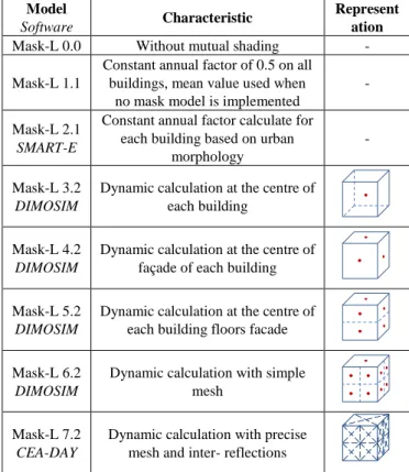
Among the abundance of models, eight different models were chosen because of their availability and/or their potential implementation in DIMOSIM and their precision/validation (Table 1). The interest of such models is first of all to compare static (models X.1) to dynamics (models X.2), and to reduce the computational time needed. The more the building is discretized, the more calculation points and ray-tracing it needs, surging the computation time.
The models 0.0, 1.1 and 2.1 are statics models with solar radiation reduction coefficient and do not take into account the geographic position of the district, while the
with N the number of sample, x the approximation’s value and xbaseline the reference’s value
5 others use dynamic calculation with the sun position through the year. Nevertheless, the SMART-E model (2.1) is using the 3CL-DPE method from the Direction de l’information légale et administrative (2012) (regulatory rule for existing buildings audit in France) in order to calculate a mean annual reduction factor from height and distance of surrounding buildings in a 500 m radius.
Table 1 : Considered shading mask models Model
Software Characteristic
Represent ation
Mask-L 0.0 Without mutual shading -
Mask-L 1.1
Constant annual factor of 0.5 on all buildings, mean value used when
no mask model is implemented
-
Mask-L 2.1 SMART-E
Constant annual factor calculate for each building based on urban
morphology
-
Mask-L 3.2 DIMOSIM
Dynamic calculation at the centre of each building
Mask-L 4.2 DIMOSIM
Dynamic calculation at the centre of façade of each building Mask-L 5.2
DIMOSIM
Dynamic calculation at the centre of each building floors facade Mask-L 6.2
DIMOSIM
Dynamic calculation with simple mesh
Mask-L 7.2 CEA-DAY
Dynamic calculation with precise mesh and inter- reflections
The models of DIMOSIM are based on ray-tracing algorithm with different discretization levels under the 1990 Perez sky model. Two discretizations are implemented in order to have an effective scan of the built environment. First, the nearer the neighbouring building is, the more discretized his footprint is, to account of their potential influence while reducing calculation time. A reduction coefficient for the direct radiation is calculated for each time step and each calculation point over 360-degrees. As for the diffuse radiation, constant sky view factors are applied. DIMOSIM solar radiation computation was compared to TRNSYS, Transient System Simulation Tool, on a single building in order to validate the simple calculation under different kinds of sky models. These comparisons showed very close results on the annual solar irradiation on each facade (under 2.5% for the isotropic model and 3.7% for the Perez model). CityEnergyAnalyst (Fonseca et al. 2015), an open source district simulator, is using DAYSIM software (Reinhart and Herkel 2000), which is validated mostly for the visual comfort. DAYSIM is based on daylight coefficients like RADIANCE (Compagnon 2001) under 1993 Perez sky model, but use a method to accelerate the computational time. This software is used in several district simulations as Strømann-Andersen and Sattrup (2011) did to assess energy consumption in a canyon street. This software is
used as first reference model and is referred as CEA-DAY.
Key comparison indicators
The solar irradiation in a district is a preliminary calculation to perform in order to calculate the solar gains, the solar potential or the micro-climate, all influencing the thermal calculation and the energy supply. Therefore, the comparison indicators for this type of models are related to the energy demand (heating, cooling, lighting), the incoming solar radiation on the roofs or facades, the thermal loads and their variations and the indoor comfort. Here for the interests of clarity and concision, only the annual heating and cooling demand and the MBE and RMSE in heating and cooling loads will be discussed.
Choice of districts
The following virtual districts are generated on the basis of a given density and random heights (Figure 1), and the typologies of Bonhomme et al. (Bonhomme, Ait Haddou, and Adolphe 2012), extended by Tornay et al. (2017), under the GENIUS project.
Figure 1: Example of a high density canyon (left) and a high density grid district (right)
All the buildings are modeled as a solely thermal zone in order to be able to take the output of solar irradiation calculation from CEA-DAY in DIMOSIM and do not then take the thermal transfer between thermal zones into account. There are no occupants, as they bring to much variability, and the buildings are powered with ideal generators and heated by ideal emitters with a 19°C set-point for heating and 26°C set-set-point for cooling. For the first simulations, a window-to-wall ratio of 0.2, an albedo of 0.2 for the ground, 0.3 for the roofs and facades are taken, with buildings N-S oriented and with U-values of 2 W/m²K for the windows and 1 W/m²K for the walls. The simulations are launch over a year with a time step of 10 min for thermal control, and 1 h for solar irradiation to match the hourly weather data.
Model selection criteria
Some model selection criteria are then created in order to detect the global characteristics of a district involving these different levels of model. Here, the criterion D*H is chosen:
𝐷∗𝐻 = ℎ
𝑚𝑒𝑎𝑛∗ 𝑑
Where hmean is the mean height and d is the district’s density (sum of the buildings’ footprints divided by the district area). But the road width could be also used.
Procedure
The solar radiation of CEA-DAY is injected in DIMOSIM to simulate the entire district with the same thermal models and systems models. The simulations are done with Paris-Montsouris 71560 (Oceanic climate) and
Athens 167160 (IWEC, Mediterranean climate) meteorological data. At the end, the other comparisons are performed only with DIMOSIM in order to avoid the compensation of errors.
Results
This section presents and analyzes the simulations previously presented. Several steps were followed:
Validation of the detailed DIMOSIM mask model compared to DAYSIM in order to use it as baseline: - On one single building
- On five districts with different shapes to see the impacts of scale and morphology
Comparison of these 5 districts with DIMOSIM as baseline
Generalization with global typologies of buildings: on three types of districts with variable heights and densities.
Comparison on one building with CEA-DAY
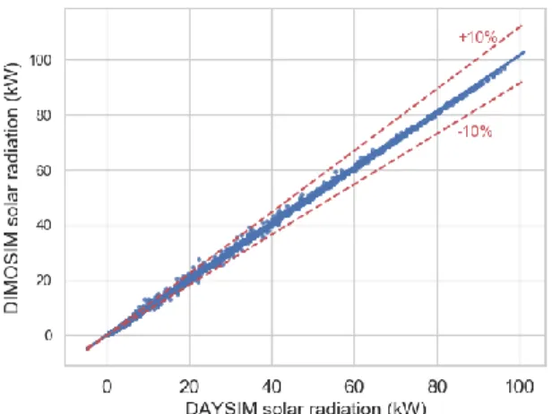
Before simulating a whole district, a simple building was considered to identify the intrinsic differences due to the calculation of solar radiation on tilted surfaces without any reflections while using the same weather data file. If the Pearson’s coefficient between DIMOSIM and CEA-DAY are very good, with the worst on the northern façade of 0.971, and the better 0.999 on the roof (Figure 2), the MBE and RMSE per orientation reach 20% (Table 2).
Table 2 : Comparison between DIMOSIM and CEA-DAY (as baseline) on solar radiation (kWh) for a simple
building
Error type East North Roof South West Total
MBErel [%] 1,5% -3,0% -15,9% -8,5% -7,8% -7,6% RMSErel [%] 3,2% 17,4% 19,1% 16,6% 15,5% 9,5%
Pearson 0.999 0.971 0.997 0.991 0.995 0.999
Figure 2 : Correlation between DIMOSIM and CEA-DAY roof solar radiation (kW) with hourly values
Most of these discrepancies are coming from the different sky models used in both simulators (Perez 1993 for CEA-DAY and Perez 1990 for DIMOSIM), mostly for the diffuse radiation, as well as the sun position that is approximated by only a set a mean values for the entire year in CEA-DAY.
To compare shading models avoiding the bias of the sky model, the radiation on shaded facades will be then
compared only on specific days where the maximal daily standard deviation upon global irradiation (direct + diffuse) between CEA-DAY and DIMOSIM is the lowest. We chose a maximal standard deviation of 10% and selected 25 days all around the year with maximal irradiation varying between 8.1 kW and 59 kW, with the 2 best days the 24/01 and 14/06 where the maximal standard deviation for all facades are under 8 %.
Comparison on five districts’ shapes
Here five types of districts are chosen:
CANYON_high and CANYON_low: Two canyon street with heights between 6 et 18m, 12 buildings and density respectively 0.6 and 0.4
GRID_high and GRID_low: two grid districts, 16 buildings with respectively heights between 21 and 65m, and 3 and 12m, and density of 0.5 and 0.15
ROW: A circle district: heights between 15 and 24m, 8 buildings
We now compare the solar radiation arriving on each building and facades for entire districts, between CEA-DAY (as baseline) and the most detailed shading-model of DIMOSIM (model 6.2). For each district two simulations are done: with and without the reflections (including the ground reflections and the inter-reflections with building, noted as R). DIMOSIM simulates the ground diffuse reflections but not the inter-reflections like CEA-DAY.
- District GRID_low
The GRID_low district, with his lower heights and density, should present a lower influence on the shading model, and so is used as a first comparison. The results are aggregated per orientation (Table 3). On the 25 selected days, the MBE for the case with no reflections, does not exceed 4%. The RMSE is mildly higher, but is still presenting good results under 6%. The solar radiation shows good correlation following the calculated Pearson’s coefficients varying between 0,989 (south) and 0,999.
Table 3 : Comparison between the solar radiation of DIMOSIM and CEA-DAY (as baseline) for each orientation of the GRID_low district for the 25 days Error type East North Roof South West Total
Without inter-reflections MBE -4% -1% 1% -4% -4% -1% RMSE 6% 5% 2% 6% 6% 3% With inter-reflections MBE -7% -4% 1% -6% -6% -3% RMSE 7% 4% 1% 7% 7% 3%
Over the entire year the errors are higher than 4%, ranging from 2% on the roof and -15% in the south for the MBE. The results were also tested on the 2 best days among the 25. The Pearson’s coefficients were slightly better but the other qualitative comparisons were marginally poorer. The 25 days were then preferred for the comparison, in order to have more variability.
With reflections, almost all errors for all facades are getting larger, certainly due to the ground diffuse reflection, since the inter-reflections aren’t much impacting with low heights and high road widths. However, the Pearson coefficients are better, with the worst value on the south of 0,993. DIMOSIM is then slightly over-estimating the lower solar radiation and under-estimating the higher ones (Figure 3), but with very little differences, and thus validating the use of DIMOSIM as baseline.
Figure 3 : Total solar radiation (KW) duration curve with hourly data, for the GRID_low district
- District GRID_high
In order to consolidate the first validation of DIMOSIM as baseline, a second simulation was undertaken with the GRID-high district. The high density and heights should imply a significant impact of masks on the solar radiation calculation.
Compared to the GRID_low district, the differences are higher (Table 4), they achieve 16% for the MBE but with good Pearson’s coefficient like the GRID_low. With the former results on the GRID_low district, an important part of the differences can be attributed to the mask model.
Table 4 : Comparison between the solar radiation of DIMOSIM and CEA-DAY (as baseline) for each orientation of the GRID_high district for the 25 days Error type East North Roof South West Total
Without inter-reflections MBE 16% 11% 16% 13% 6% 12% RMSE 17% 13% 16% 15% 9% 13% With inter-reflections MBE 14% 13% 14% 12% 10% 12% RMSE 16% 14% 14% 14% 12% 13%
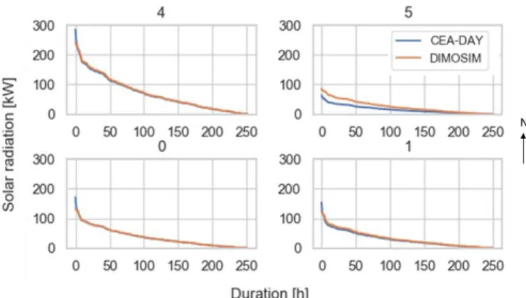
In taking into account the inter-reflections the errors decrease, it can be assumed that the error from the inter-reflections compensate the over-prediction of DIMOSIM. When looking at the building level on the two first lower rows (Figure 4), it is possible to see that DIMOSIM is underpredicting the high solar radiations when the masks don’t play a too important role on the edge of the district, but is folowwing the same tendency. For the building number 5, where the masks have the biggest impact (building situated in the middle of the district), DIMOSIM overestimates the solar radiation by more than 50% due to the shading mask model.
Figure 4 : Total solar radiation (kW) duration curve for four buildings of the GRID_high district for the selected
25 days with the inter-reflections and hourly data
The previous results show that DIMOSIM presents good agreement with CEA-DAY, even though it presents higher differences when the masks impact is important. Given the improvement of the results with the modelling of the inter-reflections, it is showed that the errors are compensating themselves between the mask models 1.1 to 5.2 and CEA-DAY. Therefore, with the good agreement between CEA-DAY and the model 6.2, it prompts us to pursue in the idea of taking DIMOSIM as baseline to simplify the comparison and avoid the compensation of errors between models.
As for the simulation time, the gain in computational time with DIMOSIM allow us to simulate multiple districts without considering the time needed for the shading masks in DIMOSIM for simple districts (Table 5). Obviously, taking real districts with buildings having plenty of facades can increase significantly the computational time compared to what is simulate here.
Table 5 : Shading mask simulation times on a i5-6200U core computer (8G RAM, CPU 2.30GHz) District Grid_high Grid_low
CEA-DAY without R 2659 s 212 s
CEA-DAY with R 3116 s 232 s
DIMOSIM 6.2 4 s < 1 s
MBE without/with R 12 / 12 % - 1 / - 3 %
In conclusion, the results in the calculation of solar irradiation and the gain in computational time between CEA-DAY and DIMOSIM allow us legitimately to take the DIMOSIM mask model 6.2 as reference.
Comparison with DIMOSIM as baseline
Since the use of the DIMOSIM mask model 6.2 as baseline is settled and validated, it is possible to assess the differences with the 5 districts created earlier. In the selected 25 days, no cooling is necessary, then here only the heating demand and the heating loads are presented. The differences between heating demands for the 5 districts are varying from -5 % to 6 % following the mask model but also the district’s morphology (ME in Table 7). As expected, for the GRID_high district, the non-modelling of masks has a more significant impact than for the GRID_low district. However, the static model 2.1 presents better results than the dynamic model 3.2 for the
GRID_high district. The model 5.2 is very close to the 6.2 with less than 1% difference, showing that the calculation here per floor’s facade is sufficient for whatever district. When looking at a more instantaneous scale, the heating power is far more affected that the heating demand (MBE and RMSE Table 7). The use of a completely random mask coefficient (model 1.1) with a rule of thumb is for the heating power too rough, even though the GRID_high district presented better results than the model 0.0 for the total heating demand. The latter is presenting good agreements even for the power demand for these 25 days on all districts. Likewise, when considering the model 2.1, its use for the GRID_high or the ROW heating consumption is well suited with less than 5% difference, but presents a difference of more than 10% when looking at the heating power. The use of one model is then dependent of the objectives and the shape of the district. The results with the Athens’ weather are not presented for the 5 districts, but only in the next results’ part.
Generalization on three types of districts
When looking at the previous results, the morphology of a district is an important matter, as well as the weather. In order to draw more generically conclusions, virtual districts are here implemented with the typology from Bonhomme et al., used previously to build the 5 districts. Here, only three types are considered together by their shape: the detached low-rise (low-rise), the detached mid-rise (mid-mid-rise) and the high mid-rise building. These types are used in order to stay in the limits of possible existing districts, and to avoid creating completely incoherent relation between heights, density or road width. For each type, 20 districts are randomly built within the range of the given parameters (min, max and mean height and road width). CEA-DAY is here not considered, in order to be able to compute heating and cooling loads all over the year.
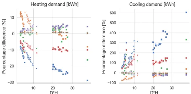
For the heating demand (Figure 5), when the districts are denser and higher, the differences are less varying, except the model 0.0 with the non-modelling of shading masks. If it is possible to say that for the heating demand and for the dense and high districts, it is sufficient to use static models like 1.1 or 2.1, or simple dynamic models like the 3.2, the use of such models implicates much higher differences in cooling demand. In contrast to the latter districts, the ones with a small D*H are presenting variable differences in a short range of indicators values. The choice of the model’s level of detail is very sensible, but stay in the reasonable range of the 10% differences for the heating demand. Nevertheless, for the cooling demand this sensitivity gives very spread results between 0 and 200 %, even reaching 500% differences for the worst cases. This is probably due to the very fast variation in the indicator between dense-low districts, and more sparse-high districts. Nevertheless, by looking at the typology of districts, it is possible to distinguish two similar trends for low value of D*H, and so be able to choose for a same value a specific model. For example, for D*H in the range of 5 to 10, the model 3.2 presents a heating demand’s MBE between -15 % and -5 %, linked respectively to a
low rise detached district and mid-rise detached district. For this latter the model 3.2 is sufficient to implement. With the Athens weather, the results are following the same trend (Figure 6), but with a different range of MBE: a smaller one for the cooling demand, and a larger one for the heating. With this spreading of results, for some high and dense districts even the use of the model 4.2 is not enough to ensure less than 10% of differences in heating demand.
Depending on the climate and the use of buildings, the wanted output will not be the same. For example, for residential buildings in Paris, where cooling devices are not often implemented, the use of simple mask models is possible for good results in heating demand without looking at the cooling part. We can then choose the adapted models for a given context. For example, if a precision of 20% on the heating demand is expected, following the criteria D*H different models can be used (Table 6).
Table 6 : Shading mask model selection for a 20% wanted accuracy in the thermal heating demand
following weather and type of district Weather District’s
type
D*H
≤ 5 [5;7[ [7;15[ [15;30[ ≥ 30
Paris
Low-rise All All - - -
Mid-rise - All X.1 - X.2 - - High rise - - - X.1 - X.2 X.1 - X.2 Athens Low-rise 4/5/6.2 4/5/6.2 - - - Mid-rise - 2.1 – 4/5/6.2 5/6.2 - - High rise - - - 3/5/6.2 X.2
The same study has to be done with the 5 other types of districts proposed in the GENIUS project, and with the inclusion of parameters variability in order to have old, refurbished or new districts with different thermal properties.
Future works
In a future work, 3 others steps will be undertaken to complete the comparison of models and draw more generic conclusion on districts types:
Step 6 – Sensitivity and uncertainty analysis
A global sensitivity analysis on multiple parameters will be done to select the most important ones involved in the analysed model. Then an uncertainty analysis is carried out with this selection on a set of representative districts, chosen accordingly to the former classification or threshold value. This will allow to see if the uncertainties are overlapping between the different models or if new conclusions must be drawn following other parameters and the available data.
Step 7 – Concatenation of sub-families
It consists in a sensitivity analysis with the models (their different levels of detail) as parameters, on a reduced set of representative districts.
Table 7 : Comparison of the thermal heating demand for the five districts under Paris weather with Mask-L 6.2 as baseline, for the 25 selected days, in percent
DISTRICT CANYON_HIGH CANYON_LOW GRID_HIGH GRID_LOW ROW
Error type [%]/
Model ME MBE RMSE ME MBE RMSE ME MBE RMSE ME MBE RMSE ME MBE RMSE
Mask-L 0.0 0 -3 12 0 -1 6 -5 -12 47 0 0 3 -1 -7 22 Mask-L 1.1 5 37 173 6 55 269 2 8 107 6 38 198 5 96 1280 Mask-L 2.1 1 3 14 1 1 5 2 10 119 0 0 3 1 16 241 Mask-L 3.2 0 0 6 1 2 6 -5 -6 42 0 0 3 0 0 86 Mask-L 4.2 1 2 11 1 1 6 1 7 90 1 1 2 1 5 52 Mask-L 5.2 0 0 3 0 0 2 0 1 8 0 0 2 0 -1 5
Figure 5 : Comparison of the thermal heating (left) and cooling (right) demands under the Paris weather for the 3 types of Bonhomme et al. districts
Figure 6 : Comparison of the thermal heating demand under the Athens weather for the 3 types of Bonhomme et al. districts
Step 8 – Application of the methodology
Simulations are performed on real districts extracted from the french digital cadaster dataset BDTOPO®, compiled by the French Geographical Institute “Institut national de l'information géographique et forestière” (IGN). This step
allows to assess the validity of the developed methodology on actual district with their morphological and parametric diversity.
Conclusion
After the choice’s validation of taking the model 6.2 of DIMOSIM as a baseline for the comparison, the results on 5 districts showed that the simplest static models (models 0.0, 1.1) are not sufficient to model the heating demand or power needs for most of the districts, but that more sophisticated one could be used (model 2.1), without more computational time needed. The choice of these models is strongly dependent of the shape and the indicator studied. When looking at the districts composed of detached buildings, it is possible to see trends in the MBE variation of buildings on an annual basis, even if for low value indicators the trends are more complicated to determine.
As the errors under both weathers of Paris and Athens are following globally the same tendency, it is then possible to draw conclusions when comparing one model to another. However, the different range of percentage differences between the two imply to stay careful in the choice of models following the maximal acceptable difference.
Nevertheless, the previous results are done with only one type of albedo, and above all do not take the variability in characteristics of building and envelope performance, namely like between renovated and old buildings, or the uncertainty of this parameters. Here only the first steps of the method are applied, excluding this part of study, that can affect strongly the conclusions. The entire application with sensitivity analysis and real districts will be investigate in a future work, allowing to correlate the outcomes related to the district morphology and the parameters of buildings.
References
Berthou, T., B. Duplessis, P. Rivière, P. Stabat, D. Casetta, and D. Marchio. 2015. ‘SMART-E: A Tool For Energy Demand Simulation And Otimization At The City Scale’. BS2015.
Bonhomme, M., H. Ait Haddou, and L. Adolphe. 2012. ‘Genius: A Tool for Classifying and Modelling Evolution of Urban Typologies’, PLEA2012.
Compagnon, R. 2001. ‘RADIANCE: A Simulation Tool for Daylighting Systems’. LESO-PB, EPFL.
Direction de l’information légale et administrative. 2012.
Modification de La Méthode de Calcul 3CL-DPE Pour La Réalisation Des DPE Introduite Par l’arrêté Du 9 Novembre 2006. https://www.legifrance.gouv.fr
Dogan, T., and C. Reinhart. 2017. ‘Shoeboxer: An Algorithm for Abstracted Rapid Multi-Zone Urban Building Energy Model Generation and Simulation’.
Energy and Buildings 140 : 140–53. https://doi.org/10.1016/j.enbuild.2017.01.030. Fonseca, J., T.-A. Nguyen, A. Schlueter, and F. Maréchal.
2015. ‘City Energy Analyst (CEA): Integrated Framework for Analysis and Optimization of Building Energy Systems in Neighborhoods and City Districts’.
Energy and Buildings 113 (December). https://doi.org/10.1016/j.enbuild.2015.11.055.
Frayssinet, L., F. Kuznik, L. Hubert, M. Milliez, and J.-J. Roux. 2017. ‘Adaptation of Building Envelope Models for Energy Simulation at District Scale’.
Energy Procedia, CISBAT 2017 International
ConferenceFuture Buildings & Districts – Energy Efficiency from Nano to Urban Scale, 122 (September): 307–12. https://doi.org/10.1016/j.egypro.2017.07.327. Han, Y., J. E. Taylor, and A. L. Pisello. 2017. ‘Exploring
Mutual Shading and Mutual Reflection Inter-Building Effects on Building Energy Performance’. Applied
Energy, Clean, Efficient and Affordable Energy for a
Sustainable Future, 185 (January): 1556–64. https://doi.org/10.1016/j.apenergy.2015.10.170. Martin, M., N. Hien Wong, D. Jun Chung Hii, and M.
Ignatius. 2017. ‘Comparison between Simplified and Detailed EnergyPlus Models Coupled with an Urban Canopy Model’. Energy and Buildings 157 (December): 116–25. https://doi.org/10.1016/j.enbuild.2017.01.078. Martínez-Durbán, M., L. F. Zarzalejo, J. L. Bosch, S.
Rosiek, J. Polo, and F. J. Batlles. 2009. ‘Estimation of Global Daily Irradiation in Complex Topography Zones Using Digital Elevation Models and Meteosat Images: Comparison of the Results’. Energy
Conversion and Management 50 (9): 2233–38.
https://doi.org/10.1016/j.enconman.2009.05.009. Miguet, F., and D. Groleau. 2001. ‘A Daylight Simulation
Tool Including Transmitted Direct and Diffuse Light’, BS2001.
Reinhart, C., and S. Herkel. 2000. ‘The Simulation of Annual Daylight Illuminance Distributions — a State-of-the-Art Comparison of Six RADIANCE-Based Methods’. Energy and Buildings 32 (2): 167–87. https://doi.org/10.1016/S0378-7788(00)00042-6. Riederer, P., V. Partenay, N. Perez, C. Nocito, R.
Trigance, and T. Guiot. 2015. ‘Development Of A Simulation Platform For The Evaluation Of District Energy System Performances’, BS2015.
Romero Rodríguez, L., R. Nouvel, E. Duminil, and U. Eicker. 2017. ‘Setting Intelligent City Tiling Strategies for Urban Shading Simulations’. Solar
Energy 157 (November): 880–94.
https://doi.org/10.1016/j.solener.2017.09.017. Strømann-Andersen, J., and P. A. Sattrup. 2011. ‘The
Urban Canyon and Building Energy Use: Urban Density versus Daylight and Passive Solar Gains’.
Energy and Buildings 43 (8): 2011–20. https://doi.org/10.1016/j.enbuild.2011.04.007. Tornay, N., R. Schoetter, M. Bonhomme, S. Faraut, and
V. Masson. 2017. ‘GENIUS: A Methodology to Define a Detailed Description of Buildings for Urban Climate and Building Energy Consumption Simulations’. Urban Climate 20 (June): 75–93. https://doi.org/10.1016/j.uclim.2017.03.002.
UIUC. 2015. ‘EnergyPlus Documentation : Engineering Reference’. US Department of Energy. https://energyplus.net