HAL Id: hal-01868297
https://hal.archives-ouvertes.fr/hal-01868297
Submitted on 5 Sep 2018HAL is a multi-disciplinary open access archive for the deposit and dissemination of sci-entific research documents, whether they are pub-lished or not. The documents may come from teaching and research institutions in France or abroad, or from public or private research centers.
L’archive ouverte pluridisciplinaire HAL, est destinée au dépôt et à la diffusion de documents scientifiques de niveau recherche, publiés ou non, émanant des établissements d’enseignement et de recherche français ou étrangers, des laboratoires publics ou privés.
2D Piezoelectric Lattice Model
Matija Novak, Eduard Marenic, Tomislav Jarak
To cite this version:
Matija Novak, Eduard Marenic, Tomislav Jarak. 2D Piezoelectric Lattice Model. 9th International Congress of Croatian Society of Mechanics, Sep 2018, Split, Croatia. �hal-01868297�
9th International Congress of Croatian Society of Mechanics
18-22 September 2018 Split, Croatia
2D Piezoelectric Lattice Model
Matija NOVAK
*, Eduard MARENIĆ
+, Tomislav JARAK
**Faculty of Mechanical Engineering and Naval Architecture, University of Zagreb
E-mails: {matija.novak,tomislav.jarak}@fsb.hr
+Institut Clément Ader, CNRS UMR 5312, Université Fédérale Toulouse
Midi-Pyrénées, INSA/UPS/Mines Albi/ISAE, France
E-mail: [email protected]
Abstract.In this contribution, the application of lattice models for the application of piezoelectric solids is investigated. Trusses are employed as lattice elements in order to model cohesion forces in the material. The regular triangular lattice with equal hexagonal unit cells is considered. In this work only the material without damage is analyzed as the first step in developing a suitable lattice model for predicting the failure behavior of the materials with strong electromechanical coupling. Appropriate techniques for defining the parameters of truss elements are derived and the influence of the parameters on the model performance is investigated. The efficiency of the proposed strategies will be demonstrated by suitable numerical example.
1 Introduction
The failure of the engineering component made of typical (passive) materials depends strongly on the microstructure of the material. In order to properly describe phenomena depending on material behavior at lower scales (e. g. microscale), like capturing the finite size of fracture process zone, modeling multiple cracks, fragmenting, etc., we can either (i) implement rather complicated procedures in the numerical continuum models [1,2], or (ii) apply numerical lattice models [1,3,4].
In the lattice models, a solid continuum is represented by a number of rigid particles, which interact through rheological elements (e.g. springs) that are used to model cohesive forces between the particles. In the numerical implementation, such connections are modelled by one-dimensional (1D) finite elements (trusses or beams) [3]. The evolution of damage inside the material is described explicitly by the breaking of the bonds between the particles. We note here that in the lattice models cohesive elements model behavior of the underlying solid while the particles serve only for the physical interpretation. Material parameters of the lattice elements are computed from the lattice geometry and the condition that the enthalpy of the lattice should be equal to the enthalpy of the underlying continuum model [3, 4].
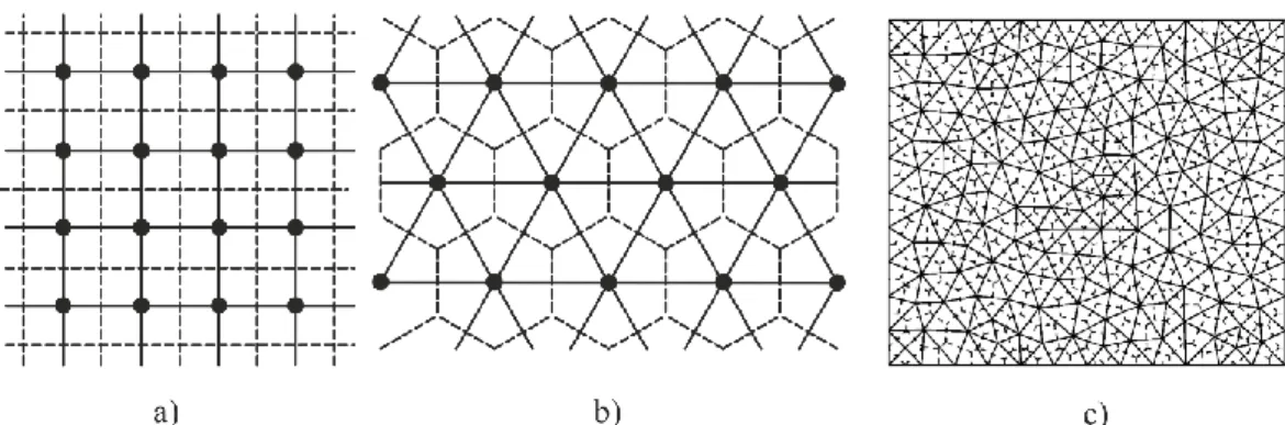
With respect to the lattice topology, two types of lattices can be distinguished: regular and irregular (see [4]). The simplest examples are square and triangular lattices shown in Figure 1. a) and b). Due to the symmetry and periodicity all lattice elements have equal geometry and material parameters (cross section area, moment of inertia, Young’s modulus, etc.). In irregular lattices, the grids are unstructured, and in general all lattice elements have different geometries, as shown on Figure 1c). The regular lattices are able to represent uniform straining exactly, while in the irregular lattices, this cannot be achieved unless different parameters are defined for each lattice element, which is not a trivial task [5]. Despite that, irregular lattices are better suited for capturing the direction
2
of crack propagation correctly and to describe the material heterogeneity at lower scales [3,4].
Figure 1: a) square regular lattice, b) triangular regular lattice, c) irregular lattice In this work, we are focusing on the piezoelectric materials. Piezoelectrics have the ability to transform mechanical to electrical energy (direct piezoelectric effect) and vice versa (inverse piezoelectric effect) [6] and are, thus, mostly used as sensors and actuators. It should be noted that, to the knowledge of the authors, this is the first attempt of modeling the piezoelectric materials by the numerical lattice models. At the moment the majority of piezoelectric materials of practical importance are brittle, thus, for the development of the new lattice model we follow similar procedures as in [4] used for the passive material. Here, we propose the procedure for establishing the lattice parameters which are computed from the condition of equality of the enthalpy of a unit cell of the lattice and the real continuum. The electromechanical coupling is included in piezoelectric constitutive relations in which stress and electric displacement both depend on strain and electric field.
2 Electro-mechanical lattice parameters
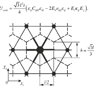
In this section we present the general framework for computing lattice parameters in a regular lattice. The presented framework is detailed for the triangular lattice, where lattice elements form equilateral triangles (see Figure 2).
2.1 General procedure
Analogously as for the passive media [3], for the active piezoelectric material the lattice parameters follow from the equivalence of continuum and the lattice unit cell enthalpy
.
cont cell
U U (1)
The enthalpy of the continuum piezoelectric media [6] reads
1 1 d d , 2 2 cont V V U
σ ε V
D E V (2)where andσ ε are the second order stress and strain tensors, D stand for the electric displacement vector and E denotes the electric field vector. Constitutive equations for piezoelectric materials are [6, 7]
– , ,
σ Cε eE D eε κE (3)
where C is the fourth order elasticity tensor, e is the third order tensor of piezoelectric coupling coefficients and κ is the second order permittivity tensor. Including the constitutive equations (3) in (2), and assuming that the strains and electric fields are constant, the enthalpy of the continuum can be written as
2
,2
cont ij ijkl kl k kij ij i ij j V
U C E e E E (4)
where V is the volume of the unit cell.
Enthalpy of the single unit cell is computed by summing up the enthalpies of all the lattice elements in this unit cell
( ) ( ) ( ) ( ) 1 1 1 d d , 2 2 e N e e e e cell e V v U V V
σ ε
D E (5)where superscript e stands for e-th lattice element and Ne denotes the total number of
lattice elements in one unit cell.
2.2 Triangular lattice with hexagonal unit cell
In what follows we limit our consideration to the hexagonal unit cells (see Figure 2),
whose volume is 2
3 / 2,
V l t with l being the length of the lattice element and t the
thickness of the unit cell. Inserting this volume into (4), we obtain for continuum
2
3
2 .
4
cont ij ijkl kl k kij ij i ij j l t
U C E e E E (6)
4
Obviously, the continuum electrical enthalpy (6) can be decomposed in three parts: the mechanical, coupled and electrical, defined by the first, second and third term of the right-hand side of the equation (6), respectively.
Herein, the truss elements are used as lattice elements, analogously to similar lattice models of passive material [3]. The key difference is that the piezoelectric trusses are used, that is, these elements have two nodes and three degrees of freedom (two displacements and the electric potential) in each node [8]. For this type of finite element, constitutive equations (3) for the e-th element reduce to simplest one-dimensional form
( ) ( ) ( ) ( ) ( ) 11 11 111 1 ( ) ( ) ( ) ( ) ( ) 1 111 11 11 1 , , e e e e e e e e e e E e E D e E (7) where ( )e
E is the Young’s modulus of the lattice element. All the components in (7) refer
to the local coordinate system of the element e, with the coordinate axis 1 in the direction of the truss element, while all the other stress, strain, electric field and electric displacement components vanish in this one-dimensional form. Plugging reduced form of the constitutive equations (7) in equation (5), and taking N e 6 yields for the lattice
6 ( ) ( ) ( ) ( ) ( ) ( ) ( ) ( ) ( ) 11 11 1 111 11 1 11 1 1 1 + d . 2 e e e e e e e e e cell e V U E e E E V
(8)In this work it is further assumed that all material parameters are constant along the truss cross section and equal for all the elements in the unit cell. The truss strain and electric fields (in each element) are obtained by projecting the global strain and electric fields on the truss axis ( )e
i
n
as ( ) ( ) ( ) ( ) ( ) 11 , 1 , e e e e e i ij j i i n n E n E (9)where ij and Ei are the global uniform strain and electric fields, respectively. Indices i
and j take values 1 or 3, depending on the direction in the global coordinate system
1 3.
OX X For the hexagonal unit cell depicted in Figure 2, the unit direction vectors read as
(1) (4) (2) (5) (3) (6) 1 1 1 1 1 1 (1) (4) (2) (5) (3) (6) 3 3 3 3 3 3 1 1 1, , – , 2 2 3 3 0, , . 2 2 n n n n n n n n n n n n (10)
Finally, taking the cross section of the lattice truss elements to be rectangular with thickness t, equal to the thickness of the continuum model, and height h equal to the side of the hexagonal unit cell (as shown in Figure 2), we can write dVA xd ,with Aht. Inserting (9) and (10) into (8), and integrating over element’s halflength, 0 x l/ 2, the final expression for the enthalpy of a unit cell may be written as
2 6 6 6 ( ) ( ) ( ) ( ) ( ) ( ) ( ) ( ) ( ) ( ) ( ) ( ) 111 11 1 1 1 3 2 . 12 e e e e e e e e e e e e cell ij kl i j k l i jk i j k i j i j e e e l t U n n n n E e n n n E E n n
(11)Analogously to the continuum, we note that the unit cell enthalpy (11) is composed of the mechanical, coupled and electrical part.
2.3 Lattice parameters for structured triangular piezoelectric truss lattice
Having the expression of the previous subsection at hand, we proceed to determine (i) mechanical, (ii) coupled, and (iii) electrical lattice parameters.
Imposing the equivalence of above developed continuum and unit cell enthalpies yields the following mechanical material parameters
( ) ( ) ( ) 1111 1133 1313 3 1 1 , , . 4 4 4 e e e C E C E C E (12)
From (12), it can be deduced analogously as for the passive materials [1,4] that for the plane stress cases the Poisson’s ratio of the proposed lattice model is fixed to the value of
1 / 3.
The Young’s modulus on the other hand is computed from the plane stress condition 1111 1 2, cont E C (13)
where Econt is the Young’s modulus of the continuum model. From (12) and (13), it
follows that the Young’s modulus for the truss lattice elements can be computed as
( ) 3 .
2
e
cont
E E (14)
Typically the piezoelectric coupling tensor has few non-zero components (see e.g. [6,9]), namely
e
311,
e
322,
e
333,
e
113and
e
223,
given that the material is polarized in direction3
.
X
Analogously as for the mechanical parameters, the piezoelectric coupling coefficients of the lattice elements are computed from the equivalence of (6) and (11), leading to( ) ( ) 311 113 111 322 223 333 111 3 3 , 0, . 6 2 e e e e e e e e e (15)
Combining the first and last term from (15) one notes the following constraints between the global model coupling parameters
311 113 333/ 3.
e e e (16)
which need to be respected for the proposed lattice model to accurately describe the behavior of the underlying continuum.
Finally, the equality of the electrical parts of the enthalpies (6) and (11) leads to
( )
11 11 33, 22 0.
e
(17)
In equation (17) there is also one constraint,1133, implying that the proposed model
6
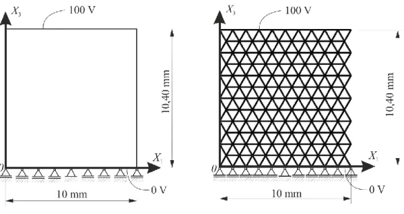
3 Numerical analysisThe performance of the developed lattice model is tested on the academic example of the uniaxial contraction of the rectangular plate due to electric charge. Mechanical boundary conditions are imposed along the bottom edge, while the electric potential is imposed on the top and bottom edge, as shown on Figure 3a).
Figure 3. Boundary conditions: a) continuum model, b) lattice model
The analytical solutions, based on the continuum model with Econt 56540 MPa, 1 / 3
and 9 2
11 33 16,50 10 N/V ,
are compared with the solution obtained by the
piezoelectric truss element lattice model presented in Figure 3b). The calculations are performed for two sets of values of the continuum coupling parameters, given in equations (18) and (19), whereby the constraints (16) are met only in the first case.
3 3 311 313 113 N N Case1: 4,32 10 , 12,96 10 , Vmm Vmm e e e (18) 3 3 311 322 333 3 113 223 N N Case 2: 21,68 10 , 12,96 10 , Vmm Vmm N 17,00 10 . Vmm e e e e e (19)
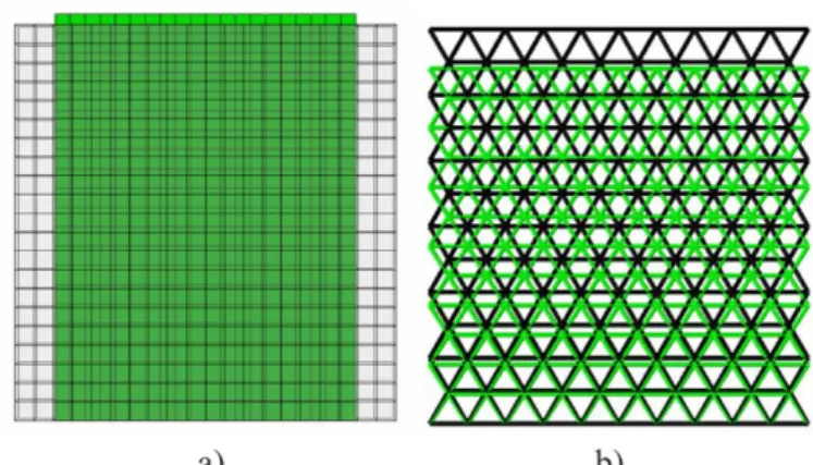
In (18) and (19), only the coupling coefficients with non-zero values are given with respect to the global coordinate system as defined in Figure 3. Displacements in both directions and enthalpies are compared with analytical results. Obtained values are presented in Table 1, while Figure 4 and Figure 5 show the undeformed and deformed shape of the continuum model and lattice model for the Case 1 and Case 2, respectively.
Table 1. Results for displacements and enthalpies for the Case 1 and Case 2
Case 1 Case 2
Analytical
solutions (l=0,25 mm) Lattice Analytical solutions (l=0,25 mm) Lattice Horizontal displacement / mm 8 7,352 10 0 5 1, 744 10 0 Vertical displacement / mm 5 2, 040 10 5 2, 037 10 6 2,386 10 5 2, 037 10 Enthalpy / Nmm 4, 606 10 5 4, 604 10 5 5, 783 10 5 4, 604 10 5 Enthalpy error, % - 0,043% - 20,39%
Figure 4. Undeformed and deformed shape for Case 1: a) continuum model, b) lattice model
Figure 5. Undeformed and deformed shape for Case 2: a) continuum model, b) lattice model It is to be noted that four different lattice models have been used in calculations, with the length of the lattice elements equal to 2 mm, 1 mm, 0.5 mm and 0.25 mm, but the results for displacements and enthalpy converged to the values presented in Table 1 even when using the coarsest model.
8
4 ConclusionIt is clearly visible that accurate results are obtained by the proposed lattice model only if the material constraints (16) are met, otherwise significant errors can be generated. While this fact significantly restricts the practical applicability of the present lattice model, it is expected that this shortcoming can be efficiently overcome by applying piezoelectric beam elements instead of the truss elements, analogously as for the passive materials [1, 3, 4].
References
[1] G. Z. Voyiadjis, Handbook of Damage Mechanics, Springer, New York, 2015. [2] M. Jirásek, Nonlocal damage mechanics, Revue européenne de génie civil, 11:
993-1021, 2007.
[3] M. Ostoja-Starzewski, Lattice models in micromechanics, Appl Mech, 55(1): 35-60, 2002.
[4] M. Nikolić, E. Karavelić, A. Ibrahimbegović, P. Miščević, Lattice Element Models and Their Peculiarities, Arch Computat Methods Eng, 2017.
[5] E. Schlangen, E. J. Garboczi, New method for simulating fracture using an elastically uniform random geometry lattice, Int J Engng Sci, 34(10): 1131-1144, 1996.
[6] V. Piefort, Finite Element Modelling of Piezoelectric Active Structures, PhD Thesis, Universite Libre de Bruxelles, 2001.
[7] J. Sladek, V. Sladek, Ch. Zhang, P. Solek, E. Pan, Evaluation of fracture parameters in continuously nonhomogeneous piezoelectric solids, Int J Fract, 145: 313-326, 2007.
[8] Simulia, Abaqus Analysis User’s Guide, 2014.