Science Arts & Métiers (SAM)
is an open access repository that collects the work of Arts et Métiers Institute of
Technology researchers and makes it freely available over the web where possible.
This is an author-deposited version published in: https://sam.ensam.eu Handle ID: .http://hdl.handle.net/10985/10563
To cite this version :
Florent COLOMBET, Damien PAILLOT, Frédéric MERIENNE, Andras KEMENY - Impact of geometric field of view on speed perception - In: Driving Simulation Conference, France, 2010-09-09 - Les Collections de l'INRETS - 2010
Any correspondence concerning this service should be sent to the repository Administrator : archiveouverte@ensam.eu
Impact of Geometric Field Of View
on Speed Perception
Florent Colombet, Damien Paillot, Frédéric Mérienne, Andras Kemeny
Arts et Metiers Paris Tech, CNRS, Le2i, Institut Image 2 rue T. Dumorey, 71100 Chalon-sur-Saône, France Technical Center for Simulation, Renault
1 avenue du Golf, 78288 Guyancourt
colombet@cluny.ensam.fr, paillot@cluny.ensam.fr, merienne@cluny.ensam.fr, andras.kemeny@renault.com
Abstract – This paper deals with changes of the geometric field of view on speed
perception. This study has been carried out using the SAAM dynamic driving simulator (Arts et Métiers ParisTech). SAAM provides motion cues thanks to a 6 DOF electromechanical platform and is equipped with a cylindrical screen of 150°. 20 subjects have reproduced 2 speeds (50 km/h and 90 km/h) without knowing the numerical values of these consigns, and with 5 different visual scale factors: 0.70, 0.85, 1.00, 1.15 and 1.30. This visual scale factor correspond to the ratio between the driver’s field of view covered by the screen (constant) and the geometric field of view. This study shows that this visual scale factor has a significant impact on the speed reached by the subjects and thus shows that perceived speed increases with this visual scale factor. A 0.15 modification of this factor is enough to obtain a significant effect. The modification of the geometric field of view remained unnoticed by all the subjects, which implies that this technique can be easily used to make drivers reduce their speed in driving simulation conditions. However, this technique may also modify perception of distances.
Résumé - Cet article présente l’effet du changement du champ de vision
géométrique sur la perception de la vitesse. Cette étude a été réalisée sur le simulateur de conduite dynamique SAAM (Arts et Métiers ParisTech). SAAM utilise une plate-forme électromécanique à 6 DDL et est équipé d’un écran cylindrique de 150° pour restituer la sensation de mouvement. 20 sujets ont reproduit 2 vitesses (50 km/h et 90 km/h), sans connaître les valeurs de ces vitesses, et avec 5 facteurs d’échelle visuelle différents : 0.70, 0.85, 1.00, 1.15 et 1.30. Ces facteurs d’échelle correspondent aux rapports entre le champ de vision du conducteur couvert par l’image (constant) et le champ de vision géométrique. Cette étude montre que ce changement visuel a un impact significatif sur la vitesse qu’atteignent les sujets et montre donc que la vitesse perçue augmente avec ce facteur d’échelle visuelle. Un changement de 0.15 de ce facteur suffit pour obtenir un effet significatif. Les changements de champ de vision
géométrique n’ont été détectés par aucun des sujets, ce qui implique que cette technique peut facilement être utilisée pour amener les conducteurs à réduire leur vitesse en conditions de simulation de conduite. Cependant, cette technique pourrait aussi modifier la perception des distances.
Introduction
Driving simulation allows car manufacturers to develop and test their future cars with digital prototypes and thus reducing the number of physical prototypes. It is thus possible to test the ergonomics, the comfort, the safety, new driving aid systems with drivers in the loop. To ensure the behavior fidelity of the drivers and thus the validity of these studies, drivers have to be provided with motion cues as close as possible with those in real conditions. That’s why a large number of human factors studies (Kemeny & Panerai, 2003) (Kennedy et al., 1993) have been carried out with driving simulators to study driver behavior or self-motion perception in driving conditions.
In this paper we will investigate more precisely speed perception. Previous studies (review in Kemeny & Panerai, 2003) show that many factors influence perception of speed, such as optic flow, time-to-contact, field of view, angular declination, image contrast or weather conditions. Perception of speed has been deeply investigated by several authors such as (Lappe et al., 1999) who claim that optic flow is the main factor for perception of self-motion. (Berthoz et al., 1975) have also shown the importance of peripheral vision for the perception of linear horizontal self-motion. According to (Jamson, 2000), the image resolution and the field of view have a significant impact on speed perception. (Panerai et
al., 2001) showed the significant influence of the height of the driver viewpoint on
perception of speed in comparison to real-world driving.
More recently, (Mourant et al., 2007) studied the influence of the geometric field of view on speed perception. In his experiment, he asked subjects to produce certain speeds (30 and 60 mph) on a static driving simulator with a 45 deg curved screen and with different geometric field of view (GFOV) conditions (25, 55 and 85 deg). He found that produced speed was highly correlated to the GFOV and that produced speed decreased when the GFOV increases. (Diels & Parkes, 2009) made a similar experiment on the TRL driving simulator (visual display covering 210 deg, vibrations rendering, no motion). Subjects were also asked to produce different speeds (20, 30, 50 and 70 mph) with four different GFOV conditions (175, 210, 245 and 280 deg). He obtained similar results.
(Mourant et al., 2007) and (Diels & Parkes, 2009) both claim that perceived speed increases linearly with the size of the GFOV. However in their studies, subjects are asked to produce and not to reproduce vehicle speeds. As speed perception depends on driving conditions (Panerai et al., 2001), in this paper we propose to investigate more precisely the impact of GFOV modifications on speed perception with a speed reproduction task. This experiment has been done with the dynamic driving simulator SAAM (Arts et Métiers ParisTech / Renault, previously referred to as SAM (Colombet et al., 2009)).
Method
Participants
Twenty volunteer subjects (3 female and 17 male) external to the lab participated in this study. They ranged in age from 20 to 69 years old (mean 44 years old). They all had 10/10 or corrected to 10/10 vision, held a valid driving license for almost 2 years (mean 25 years) and drove 26 000 km/year on average.
Driving simulator
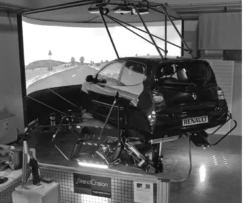
This experiment was carried out using the SAAM (referred to previously as SAM (Colombet et al., 2009), see Figure 1) dynamic driving simulator. It is composed of a cockpit based on a Renault Twingo II standard car which has been lightened and instrumented. The inside of the cockpit is unchanged so it is visually identical to the initial car.
Figure 1. SAAM dynamic driving simulator (Arts et Métiers ParisTech / Renault)
Visual environment is projected thanks to 3 DLP projectors at a 1280x1024 resolution per channel on a 150° cylindrical screen . The screen is high enough for its top not to be seen by the driver. The cockpit and the screen are interdependent thanks to a chassis that also liaise between the cockpit and the upper frame of the electromechanical platform.
Accelerations are rendered thanks to a Gough-Stewart electromechanical platform (MOOG 2000 E) which allows 6 degrees of freedom (± 20 deg, ± 0.25 m, ± 5 m/s²). A classical motion cueing algorithm with anti-backlash filters (Reymond & Kemeny, 2000) is used to compute the simulator displacements. In this algorithm, high-frequency accelerations are rendered by simulator displacements while low-frequency accelerations are rendered by tilt-coordination. Simulated vehicle vibrations are not rendered.
Haptic rendering is done on the steering wheel (active electromechanical system) and on the pedals (passive mechanical system). The gearbox is the original five speed automatic gearbox of the car. Sound of the engine, the road and the traffic is rendered through the cockpit speakers located in the doors. The whole driving simulation is generated by the SCANeR© II software (Oktal, Renault).
Surrounding parasite sounds (such as actuators noise) are cut off thanks to the cockpit which is completely closed. An intercom facility yet allows for communication between the cockpit and the control room.
Expected results
SAAM dynamic simulator differs from those used by (Mourant et al., 2007) and (Diels & Parkes, 2009) in terms of motion restitution (respectively no motion and only vibrations) and in terms of horizontal field of view cover (respectively 55° and 210°). However we expect the same result: perceived speed will grow up as geometric field of view increases.
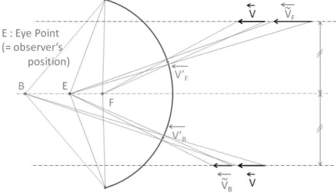
To increase the GFOV, the computational point of view is moved forward or backward to decrease the GFOV. As shows Figure 2, modifying geometric field of view will modify optic flow. The same velocity vector is displayed on the screen in if display is computed from point F and in if display is computed from point B. As the driver stays in point E, he will perceive by seeing and by seeing . And because and , and also because optic flow is one of the main factors for speed perception (Lappe et al., 1999), we can suppose that speed perception will increase (respectively decrease) when the computational point of view is moved forward (respectively backward).
Figure 2. Influence of computational point of view on both GROV and speed perception
Experimental conditions
To verify our hypothesis, five visual conditions were compared (see Figures 3 and 4). The driver’s eye-point is situated at point E. Traditionally display is computed from this same point. In our experiment, we varied the point of view used to compute the visual scene. Five different points were used: B1, B2, E, F1
and F2, all lined up along the longitudinal axis. F1 and F2 are located ahead of E,
and B1, B2 behind of E.
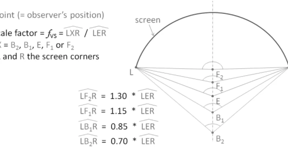
As driving simulators used by (Mourant et al., 2007) and (Diels & Parkes, 2009) do not provide the same cover of driver’s field of view, we cannot compare our results as functions of the GFOV. So we have defined the visual scale factor as the ratio between the geometric field of view and the field of view covered by the screen. The positions of points B1, B2, E, F1 and F2 have been determined
in order to obtain five different visual scale factors: respectively 0.70, 0.85, 1.00, 1.15 and 1.30.
Figure 3. Schematic presenting the different point of views in relation to the screen. Point E is the eye point, that is to say the observer’s point
of view. Display should normally be computed from point E. But for the experiment, it was computed from 5 different points: B1, B2, E, F1 and F2,
all lined up along the longitudinal axis
In every case, the computed image is displayed on the whole screen. In this way the driver’s field of view covered by the virtual scene remains identical during all the experiment.
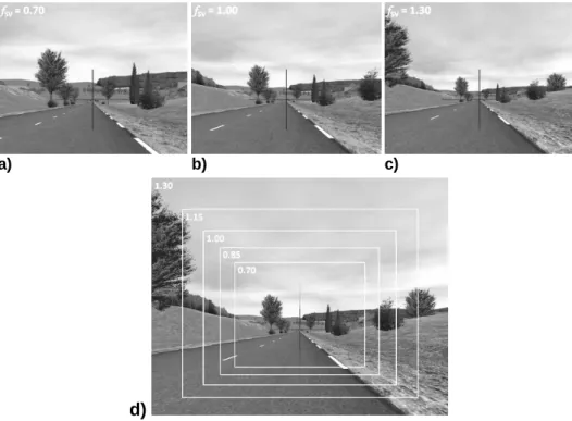
Figure 4 presents screenshots from central display with different visual scale factors, showing the effect on the computed image. The car is always at the same position for all these screenshots.
Experimental protocol
After a free practice drive to familiarize with the driving simulator, subjects were asked to reproduce two speeds (50 km/h and 90 km/h) in the 5 different visual conditions. The experiment took place on a straight country road (see screenshots in Figure 4).
a) b) c)
d)
Figure 4. Screenshots taken with visual scale factors of 0.70, 1.00 and 1.30 in respectively a), b) and c). In d), 5 screenshots (corresponding to the
5 visual scale factors 0.70, 0.85, 1.00, 1.15 and 1.30) are superposed. All these screenshots correspond to only the center image displayed in the simulator (corresponding to 52° of driver’s horizontal field of view)
For each speed and for each visual condition, subjects drove two times. First they drove with a speed regulator (cruise control) at the consign speed. Speedometer was hidden so they didn’t know the numerical value of this speed and thus no bias was introduced. The visual scale factor was then of 1.00. This first driving session lasted about 1 min.
For the second driving session, the speed regulator was disabled and the visual scale factor was randomly changed. Subjects were asked to reach the speed at which they were the first time and then to act the turn signal. The reached speed at which they felt like at consign speed was measured as soon as the turn signal was activated. Besides, as sound plays also an important role in speed perception (Kemeny & Panerai, 2003), it was disabled for this second driving session in order to see more clearly the impact of visual scale factor. Speed perception is analyzed through the speed reached by the subjects. Actually the more the speed perception grows the more the speed reached will decrease for the same perceived speed.
Each participant tested every visual scale factor with every consign speed. The order of treatment of these 10 conditions was random. Table 1 summarizes the simulator configurations for the 2 driving sessions repeated by the subject 10 times (one for each configuration in random order).
Table 1. For each of the 10 conditions (2 different consigns of speed and 5 different visual scale factors), subject had to drove 2 times. This table summarizes the simulator configurations for these two driving sessions
1st driving session 2nd driving session
Speed consign 50 km/h or 90 km/h Same as in first driving
session Visual scale factor
fSV 1.0
0.70, 0.85, 1.00, 1.15 or 1.30 randomly
Speed regulator Enabled: forced to speed consign
(not piloted by driver) Disabled
Sound Enabled Disabled
Speedometer Hidden Hidden
Motion rendering /
haptic rendering Enabled Enabled
After the experiment, subjects were asked if they noticed any changement in the simulator settings between the different driving sessions.
Results
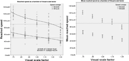
Figure 5 presents the speeds reached by the participants as a function of the visual scale factor. Values are sorted by corresponding speed consign (50 km/h in blue circles and 90 km/h in red triangles). Left graph presents all the values and right graph presents the means and the error bars representing 95% confidence level.
Figure 5. Reached speed (on the left) and mean reached speed (on the right) as functions of visual scale factor for both speed consigns (50 km/h
in circles and 90 km/h in triangles). Vertical error bars represent 95% confidence level
We can see on these graphs that as expected, speed reached by the participants is decreasing while the visual scale factor is increasing and actually means that perceived speed is increasing with the visual scale factor. This decrease seems to be done along a cubic function. Cubic regressions have been done and the R² coefficients’ corresponding to the 50 km/h and the 90 km/h consigns are respectively 0.41 and 0.574.
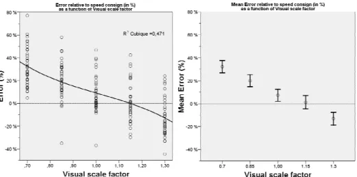
For studying at the same time data corresponding to these 2 different speed consigns, errors relative to speed consigns have been computed. Figure 6 presents the obtained values (on the left) and the corresponding mean errors (on the right) as functions of the visual scale factor. We can see that error is also decreasing along a cubic function (R² = 0.471) while the visual scale factor is increasing.
Figure 6. Error (on the left) and mean error (on the right) relative to speed consign displayed as functions of visual scale factor. Vertical error bars
represent 95% confidence level
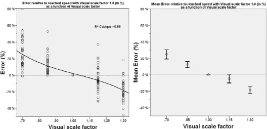
In order to study individual results, we also computed for each data the error relative to the speed reached by the same subject for the same speed consign with the visual scale factor of 1.0. We obtained the results presented in Figure 7 where we can see that this error is also decreasing along a cubic function (R² = 0.58). We can also see that there is almost no negative value for 0.70 and 0.85 visual scale factors (respectively 5% and 3%) whereas there are some positive values for 1.15 and 1.30 visual scale factors (respectively 33% and 10%). That means that relatively to the speed that subjects reached with visual scale factor of 1.0, they drove faster in 96% of the case with 0.70 and 0.85 factors. But with 1.15 and 1.30 factors, subjects drive more slowly in only 79% of the case.
A one-factor ANOVA with Tukey post hoc tests was used to analyze these error data. It showed that visual scale factor is highly significant with p < 0.001. Post hoc results show significant differences between each visual scale factor (p < 0.001) except between 1.00 and 1.15 for which we obtain p = 0.431.
Figure 7. Error (on the left) and mean error (on the right) relative to speed reached by the same subject with the same speed consign with a visual scale factor of 1.0, as functions of visual scale factor. Vertical error bars
represent 95% confidence level
To the question: “Did you notice any changement in the simulator settings
between the different driving sessions ?”, all the subjects answered they did not
notice any changement.
Discussion and perspectives
We showed that for a speed reproduction task, visual scale factor modifications significantly impacted the speed reached by the subjects, which means that speed perception increases with the visual scale factor. We also showed that a modification of 0.15 of the visual scale factor was enough to obtain a highly significant impact (p < 0.001) on speed perception. Furthermore, these visual modifications were subtle enough to remain unnoticed by drivers. So this technique can easily be employed to have drivers reduce or increase their speed in driving simulation conditions.
These first conclusions are consistent with those obtained by (Mourant et al., 2007) and (Diels & Parkes, 2009) though the task (speed reproduction instead of speed production) and the simulation conditions (dynamic with 6 DOF instead of respectively no motion and only vibrations) were different. On the other hand we also found that the variation of speed perception as a function of visual scale factor seems to be stronger when reducing the visual scale factor than when it is increased (see Figure 7). The fact that drivers seem more inclined to raise their speed rather than to reduce it could be one explanation. The absence of audio cues could also explain this result.
On the Figure 6, we can see that the error relative to the speed consign is minimum (in absolute value) for a 1.15 visual scale factor. This value is close to the result of 1.22 that (Diels & Parkes, 2009) obtain with their speed production task. In our experiment, this 1.15 value is hard to explain because the subjects were asked to reproduce a speed, and not to produce it relatively to their own real
experience. So we could have expected to find a result more close to 1.00 than 1.15. Once again, the lack of sound cues can explain this discrepancy.
Perspectives
We have seen that GFOV modification has an impact on speed perception and seems to remain unnoticed by drivers. And as speed perception is often underestimated in virtual reality applications (Banton et al., 2005), using the visual scale factor could be used for dedicated driving simulators, especially for low cost driving simulators vs. full scale driving simulators. However, the difference between the actual speed and the perceived speed seems also to depend on the speed according to (Mourant et al., 2007). So the GFOV should be dynamically changed as a function of the vehicle speed. Yet effects of dynamic variations of the visual scale factor have not been investigated and knowing the necessary conditions to keep these variations unnoticed by the drivers seems necessary. Furthermore, as acceleration is mathematically the speed derivative, dynamic variations of the GFOV may also have an effect on acceleration perception.
We can also notice that perception of distances may be affected by the visual scale factor (see Figure 2). For the driver, could be perceived “nearer” than and “farther” than . We can also see on Figure 11 that e.g. the same tree seems nearer on picture a) than on picture c). As perception of distances is important (Kemeny & Panerai, 2003) to carry out elementary driving tasks such as keeping safety distances or taking a curve, studies to determine the precise effect of the visual scale factor on perception of distances and/or on elementary driving tasks should also be considered. It could then allow concluding on the usability of this technique and to determine the conditions of experimental use.
Acknowledgements
This work has been done thanks to the support of Le Grand Chalon.
Bibliography
Banton, T., Stefanucci, J., Durgin, F., Fass, A., & Proffitt, D. (2005). The perception of walking speed in a virtual environment. Presence:
Teleoperators and Virtual Environments , 14 (4), 394-406.
Berthoz, A., Pavard, B., & Young, L. R. (1975). Perception of linear horizontal self-motion induced by peripheral vision (linearvection) basic characteristics and visual-vestibular interactions. Experimental Brain
Research , 23, 471-489.
Colombet, F., Kemeny, A., Mérienne, F., & Père, C. (2009). Motion cueing strategies for driving simulators. Proceedings of the WINVR 09
Conference. Chalon-sur-Saône, France.
Diels, C., & Parkes, A. M. (2009). Geometric Field Of View Manipulations Affect Perceived Speed in Driving Simulators. Proceedings of the Road Safety
Jamson, A. H. (2000). Driving Simulator Validity: Issues of Field of View and Resolution. Proceedings of the Driving Simulation Conference, 57-64. Paris, France.
Kemeny, A., & Panerai, F. (2003). Evaluating perception in driving simulation experiments. TRENDS in Cognitive Science , 7 (1), 31-37.
Kennedy, R. S., Lane, N. E., Berbaum, K. S., & Lilienthal, M. G. (1993). Simulator Sickness Questionnaire: An Enhanced Method for Quantifying Simulator Sickness. The International Journal of Aviation Psychology , 3, 203-220.
Lappe, M., Bremmer, F., & van den Berg, A. V. (1999). Perception of self-motion from visual flow. Trends in Cognitive Sciences , 3 (9), 329-336.
Mourant, R. R., Ahmad, N., Jaeger, B. K., & Lin, Y. (2007). Optic flow and geometric field of view in a driving simulator display. Displays , 28, 145-149.
Panerai, F., Droulez, J., Kelada, J. M., Kemeny, A., Balligand, E., & Favre, B. (2001). Speed and safety distance control in truck driving: comparison of simulation and real-world environment. Proceedings of the Driving
Simulation Conference, 91-108. Sophia Antipolis (Nice), France.
Reymond, G., & Kemeny, A. (2000). Motion cueing in the Renault driving simulator. Vehicle System Dynamics , 34, 249-259.