HAL Id: tel-02591699
https://pastel.archives-ouvertes.fr/tel-02591699
Submitted on 15 May 2020HAL is a multi-disciplinary open access archive for the deposit and dissemination of sci-entific research documents, whether they are pub-lished or not. The documents may come from teaching and research institutions in France or abroad, or from public or private research centers.
L’archive ouverte pluridisciplinaire HAL, est destinée au dépôt et à la diffusion de documents scientifiques de niveau recherche, publiés ou non, émanant des établissements d’enseignement et de recherche français ou étrangers, des laboratoires publics ou privés.
injection de bulles dans une couche limite turbulente
décollée redéveloppée
Jishen Zhang
To cite this version:
Jishen Zhang. Etude expérimentale de la réduction de trainée par injection de bulles dans une couche limite turbulente décollée redéveloppée. Autre [cond-mat.other]. Ecole nationale supérieure d’arts et métiers - ENSAM, 2019. Français. �NNT : 2019ENAM0057�. �tel-02591699�
Arts et Métiers - Campus de Paris Institut de Recherche de l’École Navale
2019-ENAM-0057
École doctorale n° 432 :
Sciences des Métiers de l’ingénieur
présentée et soutenue publiquement par
Jishen ZHANG
le 12 décembre 2019Experimental Study of the Bubbly Drag Reduction in the Recovery
Region of a Separated Turbulent Boundary Layer
Doctorat
T H È S E
pour obtenir le grade de docteur délivré par
l’École Nationale Supérieure d'Arts et Métiers
Spécialité “ Mécanique des Fluides et Énergétique”
Directeur de thèse : Jean-Yves BILLARD Co-encadrement de la thèse : Céline GABILLET
T
H
È
S
E
JuryM. Éric CLIMENT, Professeur des Universités, HMF, IMFT Président
M. Mohamed FARHAT, Professeur, STI IGM LMH, EPFL Rapporteur
M. Jean-Yves BILLARD, Professeur des Universités, IRENav, ENSAM – École Navale Examinateur
M. Antoine DAZIN, Professeur des Universités, FISE, ENSAM ParisTech Examinateur
Mme. Céline GABILLET, Maître de Conférences, IRENav, ENSAM – École Navale Examinateur
Ainsi qu’au cabaret l’homme demeure au monde. Le plaisir et le vin se laissent avaler.
Le temps y dure peu, tant que la joie abonde. Et puis il faut compter, payer et s’en aller.
m’avoir accueilli au sein du laboratoire, d’avoir soutenu et guidé depuis ma première année de thèse. Son exigence m’a enseigné la rigueur du travail, ses compétences, son expérience professionnelle et ses conseils avisés m’ont été indispensables tout au long de ces années.
Je tiens à remercier Monsieur Jean-Yves Billard, qui m’a dirigé dans cette thèse, en particulier pour la confiance et la liberté qu’il a bien voulues m’accorder. Je remercie Monsieur Eric Climent et Monsieur Mohamed Farhat pour avoir accepté la tâche de rapporteurs. Que Monsieur Antoine Dazin et Madame Gaëlle Perret soient également remerciés d’avoir participé au jury de soutenance.
Ma profonde reconnaissance va à l’équipe du service technique (SEFER) : Michel, Alain, Jean-Charles, Steve, Laurent, Pierre et Arnaud.
Special thanks to my supervisor 村井さん for having welcome me in the Flow Control Laboratory of the University of Hokkaido and allowed me to discover the artistic side of bubbles and for his kind advice during my stay in Japan. Thanks to my co-supervisors and colleagues : 田坂さん and 朴さん, 衆示さん, 俊さん, 大地さん, 侑さん, 大輝さん, 幸太郎さん, 菅野さん, 健介さん, 亦默さん, 栩 さん, 惠実さん, Suzy さん and Martina さん.
Mes pensées vont ensuite aux collègues de l’IRENav avec qui j’ai aiguisé mes connaissances sur la préparation du café presque parfait, sur les fines stratégies du jeu de tarot ou bien sur la distinction entre le vrai beurre et le faux ; Vennec et Yannick qui ont dépanné le réseau et le serveur avec leurs formules magiques ; Marie et Abdel qui m’ont accompagné quotidiennement pour traverser la Grande Porte Robert Surcouf ; Karine qui m’a donné d’excellents conseils sur les films italiens ; Vanilla ma précieuse collègue qui a supporté l’état turbulent de mon bureau pendant 3 ans avec sa gentillesse et sa bienveillance ; Loïc qui s’est vanté de ses talents de pâtissier et de ses anecdotes de « son époque » ; Joseph et Rozenn qui ont apporté de la joie de vivre et sans qui mes années de thèse n’auraient pas pu être aussi heureuses …
Mes remerciements s’adressent aussi à l’équipe de la cellule pédagogique de l’Ecole Navale, Pierre, Christophe, Alexandre, Jimmy et Jean-Yves, pour m’avoir conseillé et aidé à m’épanouir dans mon travail d’enseignant. Je remercie particulièrement à mon ami Pierre pour les nombreuses discussions intéressantes qui ont rendu les 1460 heures en bateau trans-rade beaucoup moins ennuyeuses.
Je remercie également mes amis Alice, Ségolène, Thibault, Gilles, Fatih, Owenn, François, Guillaume, Maryvonne, 池子强, 徐霄, 王乐, 尚亚菲, 石婵 et 刘泽 …
Je ne pourrais terminer sans remercier ceux qui sont chers à mon cœur, et qui m’ont toujours soutenu au cours de mes études : ma mère, mon père, mon grand-père et ma grand-mère.
i Table of Contents
Table of Contents ... i
Nomenclature ... v
1.1 Roman Symbols ... v
1.2 Greek Symbols ... vii
1.3 Abbreviations ... viii
Introduction ... 1
1 CHAPTER I. Literature Survey & Objectives ... 4
1.1 Generalities about the single-phase turbulent boundary layer ... 4
1.1.1 Equations of conservation ... 6
1.1.2 Integral length scales ... 7
1.1.3 Discussion about universality of the mean stream-wise velocity profiles ... 8
1.1.4 Discussion about universality of the turbulent shear stress profiles ... 12
1.1.5 Discussion about the mechanism of turbulence production in the turbulent boundary layer 13 1.2 Generalities about the single-phase turbulent flow downstream of obstacles at the wall ... 15
1.2.1 Classification of obstacle perturbation ... 16
1.2.2 Reattached flows ... 16
1.2.3 Turbulent structure in adverse pressure gradient flows ... 17
1.3 Bubbly turbulent boundary layer ... 17
1.3.1 Effect of the bubble size: Micro-bubbles ... 18
1.3.2 Effect of the bubble size: Intermediate-size bubbles ... 20
1.3.3 Effect of the bubble size: Single large bubbles ... 22
1.3.4 Effect of the pressure gradient ... 23
1.3.5 summary ... 24
1.4 Conclusion ... 25
2 CHAPTER II. Description of Experimental Device and Flow Conditions ... 26
2.1 Experimental Device ... 26
2.2 Flow Conditions ... 29
2.3 Experimental Techniques ... 31 2.3.1 High frequency PIV measuring system for the characterization of the single phase flow
ii 2.3.2 PTV measuring system for the characterization of the liquid phase in the two-phase
flow 34
2.3.3 Shadowgraphy measuring system for the characterization of the gas phase in the
two-phase flow... 39
3 CHAPTER III. Characterization of the Single Phase Flow Developing Downward the Step ... 46
3.1 Analysis procedures ... 46
3.1.1 Time-Averaging ... 46
3.1.2 POD analysis ... 49
3.2 Results. Characteristics of the single phase flow ... 51
3.2.1 General features of the mean flow ... 51
3.2.2 General features of the fluctuating flow ... 55
3.2.3 validity of the universal logarithmic law ... 60
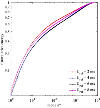
3.2.4 Modal decomposition and frequency analysis ... 66
3.2.5 Longitudinal evolution of the integral scales of the flow ... 69
3.2.6 Discussion ... 71
3.3 Conclusion ... 75
4 CHAPTER IV. Influence of Bubble Injection on the Flow Developing Downward the Obstacle. Characterization of the Gas Phase ... 76
4.1 Bubbly Flow conditions ... 76
4.2 Statistical analysis procedure of Shadowgraphy measurements ... 77
4.2.1 Spatial and time averaging ... 77
4.2.2 Uncertainties ... 79
4.2.3 Validation of measurements and statistical processing. Conservation of mass flux of the gas 79 4.3 Bubble size and shape ... 80
4.3.1 Distribution of equivalent diameter ... 80
4.3.2 Evolution of the bubble equivalent diameter with flow conditions ... 82
4.3.3 Evolution of the bubble aspect ratio with flow conditions ... 84
4.4 Gas volume fraction ... 85
4.4.1 General features of the gas volume fraction profiles ... 85
4.4.2 Self-similarity of y profiles of the gas volume fraction against the air injection rate ... 86
4.4.3 Self-similarity of y profiles of the gas volume fraction against the velocity ... 88
4.4.4 Self-similarity of the y profiles of the gas volume fraction against both velocity and air injection rate ... 92
4.4.5 Analysis of the volume fraction peak in the vicinity of the wall according to the operating conditions ( , ) ... 93
iii 4.4.6 Analysis of the integral scales of the bubble layer according to the operating conditions
( , ) ... 96
4.5 Gas phase mean flow ... 100
4.5.1 Mean stream-wise velocity profiles ... 100
4.5.2 Mean wall-normal velocity profiles ... 102
4.6 Gas phase turbulence ... 104
4.6.1 Rms stream-wise velocity ... 104
4.6.2 Rms wall normal velocity ... 106
4.6.3 Turbulent shear stress ... 108
4.7 Conclusion ... 110
5 CHAPTER V. Influence of the Bubble Injection on the Flow Developing Downward the Obstacle. Characterization of the Liquid Phase Velocity Field... 112
5.1 Bubbly Flow conditions ... 112
5.2 Statistical analysis procedure of PTV measurements ... 113
5.2.1 Spatial averaging ... 113
5.2.2 Time averaging ... 114
5.2.3 Uncertainties ... 115
5.2.4 Validation in single-phase flow of the PTV measurements of the statistical quantities by comparison to PIV ... 116
5.3 Analysis of the liquid velocity field in the bubbly flow. Comparison to the single-phase flow. 117 5.3.1 General features of the mean and fluctuating liquid flow ... 117
5.3.2 Validity of the log law ... 124
5.3.3 Integral parameters of the liquid phase flow ... 129
5.4 Discussions ... 132
5.4.1 Stream-wise velocity drift between gas & liquid ... 132
5.4.2 Wall-normal velocity drift between gas & liquid ... 136
5.4.3 Non-dimensional analysis of the gain of drag variation ... 138
5.4.4 Contribution of different mechanisms ... 140
5.5 Conclusion ... 145
6 General Conlusion ... 147
6.1 Recommendations for future investigations ... 148
7 Reference ... 150
8 Appendices ... 157
iv
8.2 Appendix B. Comparison between PTV and PIV profiles in single phase flow ... 158
8.2.1 Mean velocity components ... 158
8.2.2 Reynolds stresses ... 159
8.2.3 Logarithmic law versus inner variables ... 162
8.2.4 Logarithmic law versus outer variables ... 164
8.2.5 Comparison of the integral parameters between PTV and PIV ... 166
v
Nomenclature
1.1 Roman Symbols
Major axis of the bubble contour.
Minor axis of the bubble contour.
Additive constant in the log law.
Additive constant in the log law.
Capillary number
Cross-correlation threshold for the PMC method.
Bubble drag coefficient.
Friction coefficient.
Friction coefficient of single-phase undisturbed flow.
Lift coefficient of the bubbles.
Particle-mask window size for the PMC method.
Bubble average diameter.
Width of the bubble injection area. Reconstruct the gas flow rate.
Gas-on-liquid drag force per unit volume. Gas-on-liquid lift force per unit volume.
Froude number based on the bubble diameter and the reference velocity. Froude number based on the momentum thickness and the reference
velocity.
Reference frequency.
Vortex traveling frequency.
Standard gravity.
Clauser parameter.
Clauser parameter of single-phase undisturbed flow.
Gain factor.
Obstacle height.
Shape factor.
Moore‟s bubble drag coefficient constant.
Recirculation length.
Viscous length of the boundary layer.
Power rate of the velocity power law.
Static pressure.
Static pressure outside the boundary layer.
Gas injection rate.
Water flow rate.
Seeding particle injection rate.
vi Quasi-parallel motion threshold of the particles for the relaxation PTV
method.
Reynolds number.
Reynolds number based on momentum thickness and reference velocity.
Reynolds number based on single-phase undisturbed momentum thickness and reference velocity.
Reynolds number based on momentum thickness and friction velocity.
Neighbor particles distance threshold for the relaxation PTV method. Maximum possible displacement of the particles for the relaxation PTV
method.
Threshold on the isolated bubbles selection. Instantaneous stream-wise liquid velocity.
Instantaneous stream-wise liquid fluctuation velocity. Instantaneous stream-wise bubble velocity.
Instantaneous stream-wise gas fluctuation velocity.
Stream-wise mean liquid velocity.
External stream-wise velocity.
Stream-wise mean gas-phase velocity. Stream-wise gas-phase rms velocity.
Stream-wise mean liquid-phase velocity. Reference velocity.
Friction velocity.
Time between pulses.
Shifts of semi-logarithmic profiles caused by pressure gradient. Mean stream-wise liquid rms velocity.
〈 〉 Stream-wise Reynolds stress of the liquid flow. 〈 〉 Reynolds shear stress of the liquid flow.
〈 〉 Reynolds shear stress of the gas flow.
Instantaneous wall-normal liquid velocity. 〈 〉 Wall-normal Reynolds stress of the liquid flow. Instantaneous wall-normal liquid fluctuation velocity.
Instantaneous wall-normal bubble velocity.
Instantaneous wall-normal gas fluctuation velocity.
Wall-normal mean liquid velocity.
Wall-normal mean gas velocity.
Wall-normal gas-phase rms velocity. Mean wall-normal liquid rms velocity.
Weber number based on the reference velocity and the mean bubble
diameter.
Weber number based on the friction velocity and the mean bubble
diameter.
Stream-wise coordinate. (The origin is the beginning of the obstacle.)
vii -position of gas local maximum volume fraction.
-position where – . -position where – .
Coles‟s wake term.
1.2 Greek Symbols
Gas local surface fraction.
Gas local volume fraction.
Gas local maximum volume fraction.
〈 〉 Average gas volume fraction.
Clauser's pressure gradient parameter.
Boundary layer thickness.
Boundary layer stream-wise turbulence intensity thickness. Boundary layer wall-normal turbulence intensity thickness. Boundary layer thickness of single-phase undisturbed flow.
Gas layer thickness.
Bubble boundary thickness.
Boundary layer displacement thickness.
Single-phase undisturbed boundary layer displacement thickness.
Clauser's universal thickness.
Gas volume fraction scale length. Image scale factor.
Non-dimensional wall coordinate. (outer variable.)
Circulation.
Shear rate.
Eigenvalue of the velocity matrix for POD analysis
Dynamic viscosity.
Effective viscosity.
von Kármán‟s constant.
Fluid density.
Eigenvector of the velocity matrix for POD analysis
Surface tension.
Standard deviation of the 2D Gaussian distribution for the PMC method
Wall shear stress.
Wall shear stress without gas injection. Momentum thickness of the boundary layer.
Undisturbed momentum thickness of the boundary layer.
Kinematic viscosity.
viii Production of turbulent kinetic energy.
1.3 Abbreviations
ALDR Air Layer Drag Reduction
ANR Agence Nationale de la Recherche
BDR Bubbly Drag Reduction
CCD Charged-Coupled Device
DOF Depth of Field
DR Drag Reduction
DV Drag Variation
DNS Direct Numerical Simulation
EEDI Energy Efficiency Design Index
FDRAIHN Frictional Drag Reduction for Naval Hydrodynamics
FFT Fast Fourier Transform
IA Interrogation Area
LDV Laser Doppler Velocimetry
PIV Particle Image Velocimetry
POD Proper Orthogonal Decomposition
PMC Particle Mask Correlation
PTV Particle Tracking Velocimetry
1
Introduction
Minimizing the hydrodynamic resistance of marine vehicles has been a goal of Engineers and designers for several decades. With over of the volume of the world‟s trade carried by sea (UNCTAD 2018; IMO 2019), international maritime transport is essential for the world‟s economy and yet faces a challenge in respect to climate change: despite increases in operational efficiency for many ship classes, total shipping CO2 emissions increased from million tonnes to million tonnes
( ) from to , being responsible for of global CO2 emissions (Olmer et al. 2017).
Reducing greenhouse gas emissions is imperative. The Energy Efficiency Design Index (EEDI) regulation of the International Maritime Organisation mandates improvements in ship energy efficiency. Essentially, the EEDI requires new ships (since ) to emit less CO2 per unit of
“transport work” (gram of CO2 per tonne-mile). Ships built between and are required to be
more efficient than a baseline of ships built between and . Subsequently, ships built between and must be more efficient, and those built in or later must be more efficient than the baseline (Olmer et al. 2017).
The total drag can be separated into 3 contributions: 1) skin friction (or viscous) drag, 2) form drag, 3) wave-caused resistance. Skin friction is of particular importance for marine vehicles since the latter contributes up to of a ship‟s and of a submarine‟s total resistance (Perlin & Ceccio 2015). For a surface vessel, in the general circumstances, the skin friction drag is dominant at small Froude numbers ( ).
Therefore, skin friction reduction can result into immediate decreases in fuel consumption and consequentially gas emissions. Designers struggled since long time to minimize the overall drag while maintaining desired operational characteristics. However, the minimization of one form of resistance often leads to an increase in another. For example, the use of slender hulls can reduce both form and wave drag but may cause an increase in skin friction and a decrease in stability.
All existing DR (drag reduction) techniques can be divided into passive and active means. Successful application of passive drag reduction includes modification of the hull shape and surface coating and installation of a bulbous bow. These are techniques which do not require additional input of mass, momentum or energy to promote drag reduction. Active techniques, on the contrary, require continuous engagement of mass, momentum or energy supply to achieve DR, and primarily the skin friction reduction. The relevant methods include introducing polymers/fibres or bubble/gas into the boundary layer of the flow around the hull, addition of air layers beneath hulls etc. Among these techniques, gas-induced skin friction reduction techniques are of special interest because air injection causes no damage to the environment.
Depending on the gas flux quantities and the external velocity, air injection can result in air layer drag reduction (ALDR) or in bubbly drag reduction (BDR), accordingly. ALDR occurs when a continuous air layer separates the hull surface from the flowing liquid and it interrupts the momentum transfer from the flows to the wall (Fukuda et al. 2000; Mäkiharju et al. 2013). It is reported to lead to a local drag reduction of comparing to when air layer is absent (Elbing et al. 2013). However, to maintain such a nearly continuous layer, the required air flux is reported to be quite sensible to the solid surface‟s roughness and should be approximately proportional to the square of the free stream velocity (Elbing et al. 2008). As discussed also in Ceccio (2010), that it presents a challenging control problem to maintain the air layer during changes in navigation speed and while manoeuvring at sea
2 trials. Indeed, perturbations required larger gas flux to maintain the layer (or cavity) stable (Makiharju et al. 2010)
Some structural modifications on the hull bottom such as a cavity design (i.e.: back-ward facing step) behind the air injection allow a better control of the air layer. For flow over a rough wall, the air cavity would be more cost-effective than an air layer because a relatively low gas injection rate is required to achieve the drag reduction of the same order of magnitude as in air layer case. In contrast, for a smooth wall, higher gas injection rate would be required to establish an air cavity, comparing to that for an air layer, and the rate required to establish the air cavity was reported to depend on the travel speed (Makiharju et al. 2010).
Bubbly drag reduction (BDR), comparing to ALDR, requires bubble injection in the turbulent boundary layer and evokes much more complex mechanisms. Numerous experimental & numerical investigations have been conducted to better understand these mechanisms. Successful bubble drag reduction (BDR) was firstly discussed by McCormick & Bhattacharyya (1973) and net drag reduction reaching to was achieved on a fully-submerged axisymmetric body of in length at velocities ranging from to . Madavan et al. (1984) have carried out BDR measurements in a zero pressure gradient turbulent boundary layer and found that BDR increases with increasing gas injection rates and decreasing reference velocities (increasing gas volumetric fraction) and when buoyancy pushed the bubbles towards the wall. It was also revealed that the bubbles‟ location was important: it must be with wall units of the wall to promote effective BDR (Pal et al. 1988). Some Soviet researchers (Bogdevich et al. 1976) have observed that the drag reduction reaches its maximum at the immediate location downstream the gas injection and does not persist as bubbles move away from the wall when traveling downstream. Same was observed for bubbly drag reduction under a flat pate by Elbing et al. (2008). Some numerical investigations by means of direct numerical simulation (DNS) of turbulent bubbly flow (Lu et al. 2005) have confirmed the importance of bubbles‟ wall-normal location in BDR persistence. Unfortunately, such numerical investigations are only possible at modest Reynolds numbers.
Although much research has been done experimentally and numerically on both non-equilibrium and equilibrium adverse pressure gradient boundary layers in single phase flow (Clauser 1954; Bradshaw 1967; Townsend 1956; Skåre & Krogstad 1994; Song 2002; Castillo & Wang 2004; Aubertine & Eaton 2005), very few studies have been dedicated to bubbly drag reduction in case of pressure gradient application. The influence of the pressure gradient on the BDR has been firstly studied by
McCormick & Bhattacharyya (1973). Clark & Deutsch (1991) have conducted BDR measurements on
a fully-submerged axisymmetric body under zero, positive and adverse stream-wise pressure gradient and have revealed that a weak adverse pressure gradient helps maintaining bubbles in the buffer layer and thus leads to drag reduction at low speeds. On the contrary, a favorable pressure gradient inhibited the bubbly drag reduction.
To our best knowledge, the bubbly drag reduction has never been investigated in a reattached flow (recovery region) downstream an obstacle mounted at the wall, which induces separation of the boundary layer. This configuration can be encountered in the downstream region of a cavity at the hull. The goal of this thesis is to examine experimentally bubbles interactions with a reattached turbulent boundary layer downstream of a 2D surface-mounted squared obstacle when bubbles of intermediate-size (sub-millimetric and millimetric bubbles) are injected under favorable gravity condition at the wall in the reattached flow. different free-stream velocity conditions have been studied, and the air injection rate at the wall has been varied.
3 This dissertation consists of chapters.A brief resuming of each chapter is described as follows: Chapter 1 provides an overview of the state-of-art covering single-phase turbulent boundary layer under zero and adverse pressure gradient single-phase recovery region downstream of surface-mounted obstacles, and bubbly drag reduction mechanisms.
In Chapter 2, experimental means including the water tunnel facility, obstacle geometryare described. Flow conditions with and without obstacle and gas injection configurations are mentioned. At last, instruments and means of measurement used including high frequency Particle Image Velocimetry
(PIV), low frequency Particle Tracking Velocimetry (PTV) and high frequency Shadowgraphy are
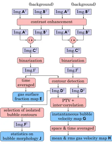
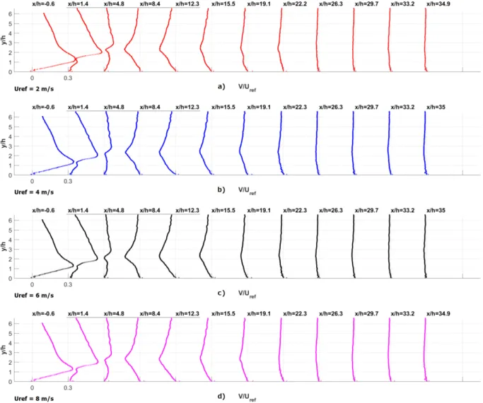
introduced, altogether with associated image processing techniques and system-induced data uncertainties. PIV was used to characterize the single phase flow at 11 stream-wise locations from the upstream of the obstacle to the recovery region, including the recirculating region. PTV and Shadowgraphy were used at one stream-wise location in the recovery region to characterize both the liquid-phase and gas-phase flows respectively under bubbles injection conditions.
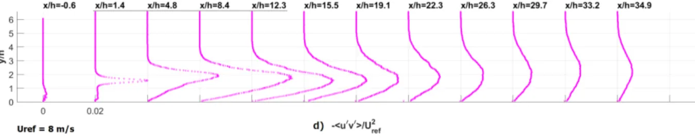
In Chapter 3, analysis procedures of experimental data of turbulent boundary layers in single-phase obstacle flow are introduced. Stream-wise evolution of integral parameters of the turbulent boundary layer in the total measuring sections, and the recirculation length are characterized. The time-averaged mean and fluctuating velocity profiles are equally presented. The influence of adverse pressure gradient on mean profiles and integral parameters is discussed and the logarithmic law of the wall of mean stream-wise velocity profiles is confirmed to be valid in recovery region.
Chapter 4 describes the gas-phase flow characteristics. The evolutions of mean bubble diameter, aspect ratio and the gas layer thickness in function of volumetric fraction, Weber number and reference velocity are illustrated and commented. The time averaged local gas volume fraction profiles are also shown and analyzed according to the air injection rate and velocity. The gas-phase mean and turbulent velocity profiles are shown and discussed in comparison with PIV single-phase profiles. The characteristics of the liquid-phase flow measured in the recovery region testing section are described in Chapter 5. Comparison is made with the single phase flow. Bubble-induced modifications in time-averaged mean and fluctuating velocity profiles, log law parameters as well as integral quantities are discussed. A return to equilibrium boundary layer and a friction velocity reduction are mentioned. Finally, the non-dimensional analysis of the bubbly flow is introduced and the mechanisms implied into bubbly drag reduction based on relative variation of the friction coefficient are discussed.
4
1 CHAPTER I. Literature Survey & Objectives
In this chapter, we describe the state of the art of the turbulent boundary layer theory, pressure gradient effects on flow structures, separated and reattached flow and bubbly drag reduction. In the first section, the general features of the single phase turbulent boundary layer under pressure gradient effect will be discussed. In the second section, generalities about separated and reattached shear flows downstream of an obstacle, mounted at the wall, will be introduced. In the last section, some principle underlying mechanisms associated with bubble-induced drag reduction will be mentioned.
1.1 Generalities about the single-phase turbulent boundary layer
Turbulence surrounds our everyday lives: from a factory chimney, to an aircraft jet; from a water flow in a river, to a tossed cup of coffee. The first known observation about turbulent flow structure was found in a sketch of Leonardo da Vinci (Figure I. 1).
Figure I. 1 “snapshot” of water flow into a tank, Leonardo da Vinci, circa 1500.
However, the problems related to the origin of turbulence, that is to say, the transition from laminar to turbulent flow, remain quite complex. It was until years later after the first illustration of da Vinci, that this phenomenon was experimentally studied by Reynolds (1883). The latter supposed that the turbulence appears as a result of a stability problem of laminar flows and its apparition was related to a definite value of the Reynolds number , where and denote the characteristic velocity and length and is the kinematic viscosity of the fluid. The Reynolds number highlights the ratio of inertia force to the friction force on the fluid particle and is a characteristic number for the similarity condition of different flows (Schlichting 1955). A large amount of experimental and theoretical investigations have been carried out between and for a deeper understanding of the laminar-turbulent transition (Dryden 1959; Schlichting 1955; Tollmien & Grohne 1961; Shen 1969; Tani 1969; Morkovin 1969; Reshotko 1976). The value of Reynolds number at which laminar-turbulent transition occurs (critical Reynolds number ) was found to vary greatly among flow types. Numerous investigations were conducted on the process of transition in the boundary layer on a flat plate (Burgers 1924; van der Hegge Zijnen 1924; Dryden 1935). The critical Reynolds number of the boundary layer developing along a flat plate (under zero pressure gradient) is expected to be ( )
, where is the distance from the leading edge of the plate. On a flat plate, in the same ways as in a pipe, the critical Reynolds number can be increased when the incoming flow is less perturbed.
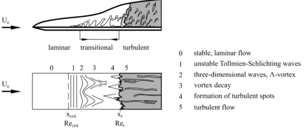
A conceptual illustration of the laminar-turbulent transition in the boundary layer is shown in Figure I. 2 (Oertel 2008). At the critical Reynolds number , 2D perturbing waves named
Tollmien-5
Schlichting waves appear in the flow and lead to characteristic 3D -vortex further downstream. The
-vortices decay and cause turbulent spots, that marks the beginning of the transition to a turbulent boundary layer flow. The transition process is complete and the boundary layer is considered fully turbulent.
Figure I. 2 Sketch of the laminar-turbulent transition in the boundary layer of a flat plate. Extracted from Oertel 2009
Figure I. 3 represents the mean stream-wise velocity distribution in the wall-normal direction achieved in a 2D fully turbulent boundary layer for stationary conditions of the flow. is the stream-wise direction, is the wall-normal direction.
Due to the presence of the solid wall, the no slip condition must hold at the wall with . For a Newtonian fluid, the wall shear stress is linked to the velocity gradient at the wall and the dynamic viscosity of the fluid
( )
denotes the external velocity outside the boundary layer. Outside the boundary layer, the flow is a potential flow. According to Bernoulli‟s equation, the external velocity is related to the static pressure outside the boundary layer.
The skin-friction coefficient is defined by:
The boundary layer thickness is by convention the distance from the wall to where the mean velocity reaches of the external velocity and increases with in the downstream direction.
6
Figure I. 3 Schematic of a wall-bounded fully turbulent boundary layer.
For reasons of dimensionality, the friction velocity can be defined as follows:
√
The friction velocity can be used to characterize the turbulent flow in the near-wall region (Chassaing 2000). It is representative of the order of magnitude of the velocity fluctuations in the turbulent boundary layer.
1.1.1 Equations of conservation
We consider a 2D stationary turbulent boundary layer. Let us denote and , the instantaneous stream-wise and wall-normal velocity components. and are the averaged velocity respectively and , are the fluctuating velocity component respectively.
Prandtl‟s boundary layer theory is of great importance to simplify the conservative equations in a
turbulent boundary layer. By introducing the following assumptions ,
,
into the averaged Navier-Stokes equations (Reynolds equations), we obtain the following differential conservation equations: -direction: ( 〈 〉 ) -direction:
Since the pressure is constant along the wall-normal direction in the boundary layer, the stream-wise pressure gradient is imposed equal to the external velocity gradient
The term 〈 〉 is the Reynolds shear stress and represents the amount of momentum in the stream-wise direction due to the correlation between the stream-stream-wise and wall-normal flow fluctuations
7 (Cousteix 1989). The total shear stress is composed of the viscous and turbulent shear stresses respectively:
〈 〉
However, in the presence of flow separation & reattachment, Prandtl‟s equation is no longer valid because some assumptions are no longer true, notably the one . That has pushed us to find a
order simplification by taking into account the following hypothesis ( ): -direction: 〈 〉 〈 〉 -direction: 〈 〉
Note that comparing to the classical Prandtl‟s momentum equation (Eq. ), two additive terms of the turbulent stress appear on the right-hand-side, which come from the contribution of stream-wise and wall-normal Reynolds stresses 〈 〉 and 〈 〉 .
1.1.2 Integral length scales
Integral length scales are length scales that characterize the boundary layer globally in the wall-normal direction. They only depend on the stream-wise position . The boundary layer is traditionally characterised by the displacement thickness , the momentum thickness, and the shape factor (Cousteix 1989). These parameters are defined in Eq. to .
∫ ( ) ∫ ( )
∫ ( ) ∫ ( )
And
The displacement thickness is a distance by which the external potential field of flow is displaced outwards as a consequence of the mass deficit in the boundary layer due to the wall. The momentum thickness quantifies the loss of momentum in the boundary layer, as compared with potential flow. These parameters are valuable because they allow the boundary layer to be characterised quantitatively, as a result, they allow informative comparisons to be made between various boundary layers under a range of scenarii.
The shape factor , being the ratio of to , is a one-parameter family of velocity profile, depending on the external pressure gradient. In the case of a flat plate, the value of the shape factor is in the laminar regime and in the turbulent regime. Clauser (1954) indicated that varies with
8 Equation , which derives from the integration in the direction of the stream-wise momentum conservation Equation , evidences that the wall shear stress is linked to the integral parameters , and the stream-wise pressure gradient
:
( )
1.1.3 Discussion about universality of the mean stream-wise velocity profiles
For the turbulent boundary layer developing along a wall, three distinct regions (inner, overlap and outer regions) can be found and two different length scales can be considered according to the distance from the wall.
1.1.3.1 Inner region:
In the inner part of the boundary layer (inner region), where the advection can be neglected, the characteristic length scale is the viscous length of the boundary layer
The normal distance from the wall can be scaled by , leading to the well-known wall coordinate (inner variable):
In the very near wall region of the inner region (i.e.: viscous sub-layer), where the viscous diffusion exceeds the turbulent diffusion, we have a linear velocity profile:
This law is well established for a very small range of ( ).
Farther from the wall, still in the inner region, where the turbulent diffusion exceeds the viscous diffusion, the mean velocity profile follows a logarithmic law.
Where denotes the universal von Kármán‟s constant and the intercept constant. For a flat plate (
), the values and are observed to be approximately independent of , despite a slight increase of with increasing (Dean 1978). It was reported that essentially depends on the roughness height (Hama 1954).
The logarithmic law versus inner variables is valid in the logarithmic region which extends for a flat plate in the range
9
Figure I. 4 Universal velocity distribution for mean velocity profiles as a function of inner variables for a turbulent boundary layer. Extracted from Clauser 1954
Much experimental work has been done over the years on modifications of the inner region under the influence of adverse pressure gradient (
) (Ludwieg & Tillmann 1950; Stratford 1959; Herring & Norbury.1967; Klebanoff & Diehl 1952; Schultz-Grunow 1941; Bradshaw 1967; Clauser 1954). Equation evidences that an adverse pressure gradient reduces the friction coefficient (Schubauer and Kebanoff 1950). Ludwieg & Tillmann (1950) have proposed an empirical formula allowing estimation of :
Where is the Reynolds number based on the momentum thickness:
Clauser (1954) showed that although the pressure gradients have a significant effect on the friction
velocity, the universal logarithmic law is well established even when pressure gradients are present (Figure I. 4) and discussed the universality of parameters and .
Direct numerical simulation (DNS) of Spalart & Watmuff (1993) indicated that the the logarithmic law may be affected by pressure gradients which can modify both the von Kármán constant and the constant. Table I. 1 summarizes the values of and obtained by diverse authors with increasing pressure gradients.
Case
Spalart & Leonard 1987 Herring & Norbury Herring & Norbury Spalart & Leonard 1987 Clauser 1954; Bradshaw 1966 Clauser 1954; Bradshaw 1966
Table I. 1 Influence of the adverse pressure gradient on inner log fit and Clauser parameters. Pressures were
normalized with
However, the functional dependency of these parameters on the pressure gradient is not known and it is also possible part of the modifications may be a Reynolds number effect. Indeed, it was reported that
10 increasing the Reynolds number in zero pressure gradient produces similar effects as increasing the pressure gradient (Spalart 1988).
Overall, the existence of a universal log law with constant and values for turbulent wall-bounded flow still remains uncertain. George (2007) argued in his resuming review that the values of in boundary layers differ from those in pipe/channel flows, and the historical value of seems to be a compromise for those flow types.
It is now to discuss the outer and overlapping regions and the effects of pressure gradient: 1.1.3.2 outer region:
In the outer part of the boundary layer (outer region), the distance from the wall can be scaled by , leading to the non-dimensional coordinate (outer variable):
In the outer region of the turbulent boundary layer, the universality of the stream-wise velocity profiles is not obvious.
The notion of “equilibrium boundary layer” is to be introduced. For an equilibrium turbulent boundary layer, profiles of as a function of are expected to be similar, regardless of the stream-wise position , Reynolds number and roughness (Clauser 1954).
Equilibrium turbulent boundary layers are very commonly examined when studying adverse pressure gradient flows. This is because once equilibrium conditions are established, the velocity profiles of the boundary layers is said self-similar and the measurements are required at only a single stream-wise position (Aubertine 2005). The study of equilibrium boundary layers has led to a greater understanding of some of the basic changes which occur to boundary layers in adverse pressure gradient.
Clauser (1954) had firstly laid out the idea of equilibrium turbulent boundary layer. For a given
equilibrium profile, some parameters should remain constant. Non-dimensional parameters were introduced, which were the ratio of the stream-wise pressure gradient to the viscous shear stress gradient over an integral length of the boundary layer.
Based on the displacement thickness, the parameter is defined as follows:
Clauser defined a new integral length scale that is easier to characterize experimentally than , and
that is considered as more universal than or .
∫ ( ) ∫
is a universal function of , depending on the value of the Clauser parameter , defined according to:
√
is approximately for a constant pressure turbulent boundary layer. Clauser indicated that under constant pressure condition, we have . For turbulent equilibrium boundary layers, a positive
11 stream-wise pressure gradient induces an increase in , and the contrary for a negative stream-wise pressure gradient (see Table I. 1).
Townsend (1961) developed another definition of equilibrium boundary layer. He pointed out that an
equilibrium layer was one in which the local rate of energy production and dissipation reached a state of equilibrium. The local energy production/dissipation was so large that the aspects of the turbulent motion were almost uniquely determined by the shear stress distribution and were independent of conditions outside the region. This assumption requires only absolute balance between energy production and dissipation but not the stress equilibrium and allows a zero pressure gradient boundary layer to be included into a family of equilibrium layer.
Equilibrium was reported (Skåre and Krogstad 1994) to be obtained when the friction coefficient remains at a low constant level of and mean velocity profiles were documented to be self-similar. Townsend (1976) pointed out that the self-similar mean velocity profiles can only be obtained if the profiles of the turbulent shear stress
are also self-similar.
Some analogue results by Cousteix (1989) on the outer region have suggested that for each equilibrium family, the corresponding deficit mean velocity profile is uniquely a function of and the function itself varies under the influence of pressure gradient parameter (Figure I. 5). It should be noticed that this observation remains true only if the Reynolds number approaches infinity, and the friction velocity approaches zero.
Figure I. 5 Self similar solutions of mean velocity profiles in the outer region of turbulent boundary layer as a function of . Extracted from Cousteix 1989
1.1.3.3 Overlap region:
The inner and outer regions are clearly separated on the condition that the Reynolds . In the overlapping region, a logarithmic law is valid.
Clauser (1954) has established the validity of a logarithm law for as a function of ,
for all equilibrium turbulent boundary layers:
Where is the shift in the additive constant of the log law from the zero pressure gradient condition.
12 increases as augments. The validity range of the logarithmic law is reduced with the increase in value: from at to at .
Figure I. 6 shows the equilibrium mean velocity profiles in the overlapping region from Clauser‟s data, the slope of the semi-logarithmic curve remains constant under different pressure gradient sets and the shift in the vertical ordinate of the straight line portion (shift in is clearly seen. As can be seen in Figure I. 6, the logarithmic region is “shortened” as the pressure gradient increases, which is in accordance with results of reattached flow of Bradshaw & Wong (1971) and Castro (1979), the latter argued that this might be due to the developing wake region.
Figure I. 6 Logarithmic plot of the mean velocity profiles versus outer variables, according to values. Extracted from Clauser 1954
At large distance from the wall, (typically of order under constant pressure), measurements diverge from the logarithmic law of the wall (Chassaing 2000). Coles (1956) has introduced the notion of a law of the wake which was an additive correction on the inner region log law (Eq. ):
Where denotes the wake term and is in the form of and the Coles wake parameter. Coles (1962) observed that equals to and becomes independent for large
Reynolds numbers ( ).
1.1.4 Discussion about universality of the turbulent shear stress profiles
Integration in the wall-normal direction ( direction) of Equation in the logarithmic region of the inner region (where advection and viscous diffusion are negligible by comparison to turbulent diffusion) yields:
〈 〉
The Reynolds stress wall-normal distributions are observed to be very sensible to the pressure gradient (Figure I. 7). With a positive increasing pressure gradient, the peak moves away from the wall (Cousteix 1989).
13
Figure I. 7 A) Reynolds shear stress profile under a mild adverse pressure gradient ( ) B) Reynolds shear
stress profile under a steep adverse pressure gradient ( ). Extracted from Cousteix 1989
Figure I. 8 shows the evolution of the total shear stress profiles under the influence of pressure gradient parameter . (As profiles are plotted in the outer region, the viscous shear stress can be neglected and the total shear stress equals approximately the Reynolds shear stress 〈 〉). It can be seen that influences the slope of Reynolds shear stress near the wall, for a negative value of , the maximum Reynolds shear stress lays in near wall region while in case of a positive value of , the
Reynolds shear stress reaches the maximum far from the wall, and the wall-normal peak location
moves away from the wall, as increases.
Figure I. 8 Self similar solution in the outer region of the wall-normal distribution of Reynolds shear stress under the
influence of Extracted from Cousteix 1989
1.1.5 Discussion about the mechanism of turbulence production in the turbulent boundary layer
For the turbulent boundary layer under constant pressure, the production of turbulent kinetic energy 〈 〉 is maximum in a sub-region of the inner region, where the contribution of turbulent diffusion is same order as the one of the viscous diffusion (buffer layer). The buffer layer is located in between the viscous sub-layer and the logarithmic region.
Some observations in the buffer layer of a smooth wall-bounded turbulent boundary layer have been made that attest for the existence of instantaneous vortices associated with strong turbulent stress events (Sheng et al. 2009).
Under the effect of instability (i.e.: an initial perturbation), a span-wise vortex that lifts locally vertically from the wall, breaks and gives birth to two elongated counter-rotating stream-wise vortices. Between the two vortices, the flow is subjected to an outflow jet “ejection” resulting in a local wall shear stress decrease (the wall stress minimum is located beneath the vortex roll up region); on the
14 other hand, wall shear stress maximum develops on the outer sides of the stream-wise vortex pair, corresponding to a “sweeping” phenomenon (inflow jet). Figure I. 9 illustrates this scenario. The vortices (coherent structures) are localized in the buffer region , their size is of the order of . It leads to instantaneous stream-wise wall shear stress streaks that alternate between minima and maxima.
Figure I. 9 Conceptual sketch of the creation of wall shear stress streaks according to vortices generation in the buffer layer. Extracted from Sheng et al. 2009
Near wall distributions of turbulent stresses for a zero pressure gradient turbulent boundary layer are shown in Figure I. 10, according to the measurements by Sheng et al. (2009). The stream-wise term reaches a maximum value in a region very close to the wall, roughly at (buffer layer). The transverse component increases gradually as increases and reaches a maximum value of . According to the continuity equation, should be observed to decreases as increases when , but such behavior is impossible to be verified experimentally (Hinze 1975). As for the Reynolds shear stress 〈 〉, a constant value in the range is observed. Following the Reynolds number or the geometry (e.g.: weak secondary flows that occur in square ducts (Kawahara 1995; Kline et al. 1967)), locations of peak production and magnitudes might be varying.
Another observation is the anisotropy of the distribution of and for flat plate turbulence.
Wilcox (1994) suggested that the two terms in the logarithmic region follows the ratio
. At a certain distance from the wall near the boundary layer upper limit, turbulence becomes isotropic, which means that the turbulent stresses in both directions are equal to each other (Schlichting 1955).
15
Figure I. 10 Universal distribution for mean turbulent shear stresses, normalized by or , as a function of inner variables for a turbulent boundary layer. Extracted from Sheng et al. 2009
Measurements of Skåre & Krogstad (1994) on a non-separated flow under strong adverse pressure gradient have shown that the distribution of kinetic energy between the different turbulent stresses remains unaffected by the pressure gradient, same ratio between the different turbulent stresses is conserved comparing to that of zero pressure gradient flows.
1.2 Generalities about the single-phase turbulent flow downstream of obstacles
at the wall
In the framework of the current study, we have focused on a specific flow with adverse pressure gradient which is a turbulent flow in the reattached region downstream of a 2D squared obstacle. The sudden restriction and expansion of the flow section makes the flow quite complex, comparing to flows without separation. This section is devoted to the description of general features of the flow developing downstream of obstacles at the wall. We are interested in the particularities of this flow that make the turbulent boundary layer different from the classical turbulent boundary layer with adverse pressure gradients (as described in section of the chapter).
Figure I. 11 shows the configuration. A separation of the boundary layer occurs, which leads to the development of a recirculating region. Here is the initial boundary layer at the obstacle position without the presence of the obstacle. denotes the recirculation length and is strongly affected by the initial inclination of the dividing streamline and thus by the obstacle‟s geometry (Bergles 1983). However, the recirculation length is reported to vary weakly with the Reynolds number (Song and Eaton 2004). The same authors have also concluded that boundary layers at less than can not be considered fully turbulent.
As shown in Figure I. 11, downstream of the recirculating region, a new shear layer is born and spreads outwards the original shear layer. At the reattachment point, the new shear layer splits and gives birth to a new sub-boundary layer.
16
Figure I. 11 Schematic of flow over obstacle
Under these circumstances, conventional boundary layer calculation methods might be inapplicable under the perturbation effects on the turbulence structure. Bradshaw & Wong (1971) suggested that it was needed to define three strengths of perturbation applied to an initial shear layer flow over obstacle. The levels were characterized by the ratio of the initial boundary layer thickness and the obstacle height .
1.2.1 Classification of obstacle perturbation
According to Bradshaw & Wong (1971), the strength of the perturbation depends on how far the new shear layer bordering the recirculation flow has spread into the original shear layer and can be classified as follows:
1) Weak perturbation: 2) Strong perturbation: 3) Overwhelming perturbation:
It was mentioned by the same authors that the flow structure might be easier to understand when it is under an overwhelming perturbation since this type of flow is less dependent on the initial boundary layer. Comparing to a backward-facing step flow, the flow over obstacle can be more complex as it involves two separation regions.
1.2.2 Reattached flows
The flow quite after the reattachment point differs much from a plane mixing layer (ordinary boundary layer), even at positions far downstream of the obstacle (Bradshaw and Wong 1971). As mentioned earlier, the split of the new shear layer at the reattachment point has resulted in roughly one-sixth of the mass flow deflecting up-stream in the case of a backward-facing step flow (Etheridge & Kemp 1977). Coles (1956) defined the reattached mean velocity profiles as a linear combination of the logarithmic law of the wall and the law of the wake.
However, it was reported in the works on reattached flow downstream of a 2D surface mounted square under a “weak” perturbation ( ; ) by Antoniou & Bergeles (1988) that the logarithmic law (Eq. ) holds true in the reattached flow, even at region near the reattached point (Antoniou & Bergeles 1988). Song & Eaton. (2002) carried out LDA & PIV measurements on separated and recovered blow with strong perturbation due to a smoothly contoured ramp and found that the logarithmic law of the wall is valid downstream of reattachment but the range of validity reduced to at but extended to at . The return of parameter and Clauser parameter to their expected values at equilibrium has been be equally observed for a reattached flow under strong perturbation at distance from the obstacle (Antoniou & Bergeles 1988).
17 1.2.3 Turbulent structure in adverse pressure gradient flows
Castro & Haque (1987) pointed out in their works on turbulent structure in the recirculation region that the turbulent structure of the separated shear layer differs from that of a plane mixing layer, notably the monotonous increase of the Reynolds normal stresses as reattachment is approached.
Agelinchaab & Tachie (2008) have carried out experimental investigations of channel flow over a 2D
square obstacle and reported that the Reynolds stream-wise, wall-normal and shear stresses increase along the dividing streamline, reach the maxima and decreases as the reattachment approaches.
Bradshaw and Wong (1971) explained that the Reynolds stresses decrease is induced by the splitting
of large eddies that produce the shear stresses. Partially in the recirculation region and after the reattachment point, values of 〈 〉 are reported to increase linearly with near the wall (Etherridge and Kemp 1977, Agelinchaab & Tachie 2008). Downstream of reattachment point where a new sub-boundary layer develops, the locations of peak values of 〈 〉 increasingly move away from the wall, under effect of the mixing and spreading of the new layer, values of maxima of 〈 〉 decrease rapidly (Agelinchaab & Tachie 2008).
In the reattached boundary layer, a stress equilibrium layer was defined (DeGraaff & Eaton 1999) as a near wall region where the Reynolds stresses are in equilibrium with the local skin friction. Song &
Eaton (2004) suggested that in the recovery region of the separated turbulent boundary layer, the inner
part of the boundary layer ( ) recovers more rapidly than the outer layer and develops a stress equilibrium layer while the energetic large eddies in outer layer persist. Accordingly, in the stress equilibrium layer, the scaling of the Reynolds stress proposed by DeGraaff & Eaton (2000) for a flat-plate turbulent boundary layer is still valid.
1.3 Bubbly turbulent boundary layer
Most of the studies dealing with the interaction between bubbles and a turbulent boundary layer have been focused on bubbly drag reduction (BDR). As mentioned in the general introduction, bubbly drag reduction has been mainly addressed in the context of propulsion of marine underwater vehicles and surface ships (Ceccio 2010).
Up to the nineties, studies dedicated to the bubbly drag reduction were experimental studies conducted in turbulent boundary layers developing at zero pressure gradient condition and small Reynolds numbers. In most of these studies, global measurement of the bubbly drag induced reduction was achieved and it reveals a large discrepancy between the results according to the Reynolds numbers and the air injection rates. When compiling all these results, even at high Reynolds numbers, self-similar laws cannot be evidenced (Sanders et al. 2006) and are still of interest. Although some physical mechanisms are suspected in the bubbly drag reduction process, it still requires academic and numerical studies, particularly local studies, to clearly identify which of the mechanisms is dominant and find, if possible, models.
We will now discuss of the different physical mechanisms implied in the bubbly drag reduction (BDR).
Park (2016) has suggested a classification of effects of bubbles in boundary layer into two categories,
passive static effects and active dynamic effects.
The passive static effects are characterized by modifications of fluid properties by small bubbles comparing to the boundary layer thicknesses. Such modifications include the decrease of near wall average density (Elbing et al. 2008) and the modification of the local viscosity (Einstein 1906). It requires a gas volume fraction peak near the wall. Madavan et al. (1985) have confirmed, in their
18 work with numerical modelling of bubbly boundary layer by locally varying density and viscosity, a quite good agreement with the experimental results.
The gas volume fraction peak is enhanced at low velocity, high air injection rate and favorable gravity direction (i.e.: injection under a wall) (Madavan 1985). Nevertheless, the gas volume fraction peak localisation in the buffer layer or in the logarithmic region depends on the bubble size and obviously plays a role.
The active dynamic effects, on the other hand, involve the modifications of the turbulent flow structure induced by the bubbles, splitting of the bubbles (Meng & Uhlman 1989)and deformation of the bubbles (Kitagawa et al. 2005).
Overall, mechanisms involved in both effects for bubbly drag reduction seem to be the issue of bubble size. Let‟s call the equivalent bubble diameter. It can be classified roughly into three types of bubble size: micro-bubble, intermediate-size bubble and large-size bubbles. This will be introduced separately along with influence on BDR. We will examine only the case when gravity is favorable to
BDR. A schematic diagram of the bubbly flow is shown in Figure I. 12.
Figure I. 12 Schematic representation of the bubbly turbulent boundary layer with gravity effect in favor of bubbly drag reduction
Let us define the gain factor as the ratio of Relative Drag Reduction (by comparison to the single phase flow) to the average gas volume fraction 〈 〉 in the bulk flow:
〈 〉
Where denotes the drag reduction as bubbles are injected and is the initial drag without bubbles. The gain factor evaluates the sensitivity of the drag reduction per unit void fraction (Murai 2014). 1.3.1 Effect of the bubble size: Micro-bubbles
A bubble is classified as a micro-bubble when its diameter is smaller than the near wall coherent structures.
In turbulent boundary layer flow, the buffer layer is extended roughly from to viscous length and is the region of high Reynolds stress, turbulent production and momentum transfert. To achieve BDR with micro-bubbles, bubbles must be able to interact with the flow structure in this region and must be smaller than the near wall stream-wise vortices responsible for the wall friction streaks (size ) (see Figure I. 9). For micro-bubbles, the magnitude of the gain can be several hundreds.
19 Recent DNS results (Ferrante & Elghobashi 2003) highlighted a large DR by bubbles with dimensionless diameter . At this size range, bubbles were reported to be trapped into the near wall stream-wise vortices of the buffer layer and created a local positive convergence ⃗⃗⃗ ⃗⃗ , resulting in a push-away effect on the vortical structures, enhancement of the outflow jet and reduction of the global viscous drag (Figure I. 13). The mechanism is a compressibility effect. At higher
Reynolds number, the stream-wise vortices are squeezed and a higher volume fraction is required to
achieve same relative reduction of the viscous drag as for smaller Reynolds numbers (Ferrante & Elghobashi 2005).
However, producing such flow is difficult experimentally because the near wall vortices are very small.
Figure I. 13 Schematic of the drag reduction mechanism in a micro-bubble turbulent boudary layer. A) single-phase flow. B) bubbly flow. Extracted from Ferrante & Elghobashi (2004)
Experimental studies of micro-bubbles injection into turbulent boundary layer on both flat plate (Madavan et al. 1984; Pal, Merkle & Deutsch 1988) and on axisymmetric bodies (McCormick & Bhattacharyya 1973; Deutsch & Pal 1990; Clark III & Deutsch 1991) were performed.
A substantial reduction of the momentum flux has been experimentally obtained in the inner region with micro-bubbles of mean diameter , which is of the order of the smallest turbulent scale (Kolmogorov length scale), leading to a local wall friction decrease by (Jacob et al. 2010). The drag reduction is associated to a loss in the coherence of the turbulent structures of the buffer layer and a redistribution of the turbulent kinetic energy in favor of the small scales of the turbulence.
In the experiments of Hara et al. (2011) and then in the experiments of Paik et al. (2016), the reduction of the wall friction is closely linked to the reduction of the turbulent shear stress induced by the important vertical fluctuating motion of the bubbles and their high concentration in the buffer layer. The flow relaminarization caused by the change in the rheological properties of the fluid in the presence of micro-bubbles can be another mechanism. Derived from the formulation of Einstein (1906) for a dilute suspension and taking into account the bubble deformability by the shear stress (Frankel & Acrivos 1970), the effective viscosity of a dispersed bubbly flow can be estimated by the following relationship: