Fast Modeling of Radiation and Conduction Heat Transfer and application example

(1)

HAL Id: pastel-00958292

https://pastel.archives-ouvertes.fr/pastel-00958292

Submitted on 12 Mar 2014

HAL is a multi-disciplinary open access

archive for the deposit and dissemination of sci-entific research documents, whether they are pub-lished or not. The documents may come from teaching and research institutions in France or abroad, or from public or private research centers.

L’archive ouverte pluridisciplinaire HAL, est destinée au dépôt et à la diffusion de documents scientifiques de niveau recherche, publiés ou non, émanant des établissements d’enseignement et de recherche français ou étrangers, des laboratoires publics ou privés.

Fast Modeling of Radiation and Conduction Heat

Transfer and application example

Boutros Ghannam

To cite this version:

Boutros Ghannam. Fast Modeling of Radiation and Conduction Heat Transfer and application exam-ple. Other. Ecole Nationale Supérieure des Mines de Paris, 2012. English. �NNT : 2012ENMP0106�. �pastel-00958292�

(2)

présentée et soutenue publiquement par

Boutros GHANNAM

le 19 Octobre 2012

Modélisation Ultra-rapide des Transferts de Chaleur par Rayonnement et par

Conduction et exemple d'application

Fast Modeling of Radiation and Conduction Heat Transfer and application

example

Doctorat ParisTech

T H È S E

pour obtenir le grade de docteur délivré par

l’École nationale supérieure des mines de Paris

Spécialité “Energétique”

Directeur de thèse : Denis CLODIC Co-encadrement de la thèse : Maroun NEMER

Jury

M. John R. HOWELL, Prof., Mechanical Eng. Department, University of Texas at Austin Rapporteur M. Olivier GICQUEL, Prof., Laboratoire EM2C, Ecole Centrale Paris Rapporteur M. Ludovic FERRAND, Dr., Technology officer, CMI Greenline Europe Examinateur M. Walter YUEN, Prof., Academic Development, The Hong Kong Polytechnic University Examinateur M. Denis CLODIC, Directeur de recherche émérite, Mines ParisTech Examinateur M. Maroun NEMER, Dr., Centre Energétique et Procédés, Mines ParisTech Examinateur

Ecole doctorale n° 432 : Sciences des Métiers de l'Ingénieur

T

H

E

S

E

MINES ParisTech

Centre Efficacité énergétique des Systèmes 60 bd Saint-Michel 75272 PARIS Cedex 06

(3)

(4)

ACKNOWLEDGMENTS

This work was carried out at the “Center for Energy and Processes – Paris” (CEP) of the “École Nationale Supérieure des Mines de Paris” (ENSMP) in France.

I first thank my supervisor Pr. Denis Clodic for hosting me in his team and advising me throughout this work. I particularly thank him for his trust and his invaluable always just in time intervention and support.

I thank Dr. Maroun NEMER for his support and guidance. His integral view on research and continuous enthusiasm for always getting better results has pushed this work forward more than I have expected.

I thank Dr. Khalil El KHOURY for his guidance and his great effort for revising and verifying the work throughout the thesis. I also particularly thank him for his enthusiasm and encouragement that always helped me to keep going forward.

I thank Pr. Walter W. Yuen for his support and effort for reviewing a part of this work. I owe him a particular acknowledgment for his work that is the basis for this thesis project.

The work presented in this dissertation was supported and partially funded by CMI INDUSTRY Thermline. I particularly thank Dr. Ludovic Ferrand and Mr. Jean-Christophe MITAIS for all the interest they have shown in this work and also for their valuable support and remarks.

I would like to express my sincere appreciation and gratitude to Anne-Marie Bonnet for her professional support and personal involvement and encouragement throughout this work. I owe her special thanks for her great effort in proofreading my work and making sure that everything goes right.

I also thank Rocio VALDEZ, Marie-Astrid KRAMES, Philomène ANGELOSANTO, and Joëlle ANDRIANARIJAONA for their professional support.

Finally, I thank my colleagues and coworkers in the CEP for their friendship, support and valuable discussions.

I dedicate this work to my parents Dunia and Georges, to my brothers Boulos, Andros, and Angelo and to my girlfriend Abeer. I particularly thank them for their support and encouragement and for enduring my absence during this work.

(5)

(6)

CONTENTS i

INTRODUCTION 1

CHAPTER 1 DIRECT EXCHANGE FACTORS COMPUTATION METHOD

9

Nomenclature Erreur ! Signet non défini.

1.1 Introduction

1.2 Multiple Absorption Coefficient Zonal Method (MACZM)

1.2.1 Concept of Generic Exchange Factors (GEF) and Superposition 1.2.2 Mean Beam Length (MBL) and Artificial Neural Network Correlations

1.3 Modray Tool Description Erreur ! Signet non défini.

1.3.1 Calculation of Direct Exchange Factors sisj with the Flux Planes Method

1.3.2 Calculation of Surface-Volume and Volume-Volume Direct Exchange Factors using Emery Et Al. Relations

1.3.3 Calculation of Total Exchange Factors using the Plating Algorithm

1.4 Elementary Operations Validation Erreur ! Signet non défini.

1.5 Test Case Description Erreur ! Signet non défini.

1.5.1 Furnace Description Erreur ! Signet non défini.

1.5.2 Modeling Approach Erreur ! Signet non défini.

1.5.3 Test Procedure Erreur ! Signet non défini.

1.6 Calculation of Radiative Exchange Factors Erreur ! Signet non défini.

1.6.1 Calculation of the Direct Exchange Factors in the Furnace using MACZM Erreur ! Signet non défini.

1.6.2 Calculation of the Direct Exchange Factors using Modray Erreur ! Signet non défini.

1.6.3 Comparison of Results And Discussion Erreur ! Signet non défini.

1.7 Experimental Validation Erreur ! Signet non défini.

1.8 Conclusions Erreur ! Signet non défini.

References Erreur ! Signet non défini.

CHAPTER 2 IMPLEMENTATION AND PARALLELIZATION OF MACZM

11

2.1 Introduction Erreur ! Signet non défini.

2.2 Multiple Absorption Coefficient Zonal Method (MACZM) And Algorithm Erreur ! Signet

non défini.

2.3 Grid Generation And Representation Of The Objects In The Discrete Space Erreur ! Signet non défini.

2.4 Mean Absorption Coefficient Computation By Ray Tracing Erreur ! Signet non défini.

2.4.1 Connectivity of The Discrete Line Erreur ! Signet non défini.

2.4.2 Span by Span Algorithm Erreur ! Signet non défini.

2.4.3 The Tripod 6-Line Algorithm Erreur ! Signet non défini.

(7)

ii CONTENTS

2.4.5 Comparison of the Ray Traversal and Mean Absorption Coefficient Computation Algorithms

Erreur ! Signet non défini.

2.5 Artificial Neural Network And GEF Superposition Erreur ! Signet non défini.

2.6 GPU Cuda Programming Model Overview Erreur ! Signet non défini.

2.7 Parallel Implementation of MACZM in CUDA Erreur ! Signet non défini.

2.7.1 Cuda Parallel Kernel Erreur ! Signet non défini.

2.7.2 Computation of The Mean Absorption Coefficient Erreur ! Signet non défini.

2.7.3 Artificial Neural Networks Erreur ! Signet non défini.

2.8 Application: Simulation of a Steel Reheating Furnace Erreur ! Signet non défini.

2.8.1 Description of The Steel Reheating Furnace and the Simplified Furnace Erreur ! Signet non défini.

2.8.2 Simulation in MODRAY Erreur ! Signet non défini.

2.8.3 Simulation in MACZM Erreur ! Signet non défini.

2.8.4 Relative Error Erreur ! Signet non défini.

2.8.5 Discussions and MACZM Multi-Grid Erreur ! Signet non défini.

CHAPTER 3 TOTAL EXCHANGE FACTORS COMPUTATION BY NRPA

13

3.2 Plating Algorithm Mathematical Formulation Erreur ! Signet non défini.

3.2.1 Matrix Representation And Parallel Execution Of The PA Erreur ! Signet non défini.

3.3 Formulation of the Non-Recursive Plating Algorithm (NRPA) Erreur ! Signet non défini.

3.3.1 Identification of the Non-Recursive Plating Algorithm (NRPA) Equation Erreur ! Signet non défini.

3.3.2 Nrpa Equation for an Enclosure With 3 Surfaces Erreur ! Signet non défini.

3.3.3 Nrpa Equation for an Enclosure With N Surfaces Erreur ! Signet non défini.

3.3.4 Demonstration of the Non-Recursive Plating Algorithm (NRPA) Equation By RecurrenceErreur !

Signet non défini.

3.3.5 Computation of the skskk − Exchange Areas Erreur ! Signet non défini.

3.3.6 Order of the Non-Recursive Plating Algorithm Erreur ! Signet non défini.

3.4 Matrix Form of the NRPA Erreur ! Signet non défini.

3.4.1 NRPA of Order 2 Erreur ! Signet non défini.

3.4.2 NRPA of Order M > 2 Erreur ! Signet non défini.

3.5 Reducing The Computational Complexity of the Nrpa Via Matrix Multiplication Erreur !

Signet non défini.

3.5.1 Overview of Matrix Multiplication Optimal Algorithms Erreur ! Signet non défini.

3.5.2 Computational Complexity of the NRPA Erreur ! Signet non défini.

3.6 Testing The Error of Non-Recursive Plating Algorithm Erreur ! Signet non défini.

3.6.1 Enclosure Description Erreur ! Signet non défini.

(8)

CONTENTS iii

3.6.3 Error Analysis and Discussions Erreur ! Signet non défini.

3.7 Implementation and Computation Time Comparison of the Pa And The Nrpa Erreur ! Signet non défini.

3.7.1 Multi-Core Cpu Implementation of the Pa Erreur ! Signet non défini.

3.7.2 Gpu Cuda Parallelization of the Pa Erreur ! Signet non défini.

3.7.3 Cpu and Gpu Implementation of the Nrpa Erreur ! Signet non défini.

3.7.4 Computation Time Comparison Erreur ! Signet non défini.

CHAPTER 4 3D HEAT DIFFUSION COMPUTATION

15

4.2 Discrete Approximation Of The 3d Heat Diffusion Equation By Finite Differences

Erreur ! Signet non défini.

4.2.1 Three-Dimensional Heat Diffusion Equation Erreur ! Signet non défini.

4.2.2 Discretization of The Heat Diffusion PDE Erreur ! Signet non défini.

4.2.3 Simple Explicit Method Erreur ! Signet non défini.

4.2.4 Simple Implicit Method Erreur ! Signet non défini.

4.2.5 Crank-Nicolson Method Erreur ! Signet non défini.

4.3 Finite Differences Split Methods Applied to the 3d Heat Diffusion PDE Erreur ! Signet non défini.

4.3.1 Locally One-Dimensional (LOD) Method Erreur ! Signet non défini.

4.3.3 Douglas-Gunn Alternating Direction Implicit (ADI) Method Erreur ! Signet non défini.

4.3.4 Alternating Direction Explicit (ADE) Method Erreur ! Signet non défini.

4.4 Highly Efficient Tridiagonal Linear System Solvers Erreur ! Signet non défini.

4.4.1 Thomas Algorithm Erreur ! Signet non défini.

4.4.2 Cyclic Reduction (CR) Algorithm Erreur ! Signet non défini.

4.4.3 Parallel Cyclic Reduction (PCR) Algorithm Erreur ! Signet non défini.

4.5 Gpu Cuda Programming Model Overview Erreur ! Signet non défini.

4.5.1 Maximizing The Number of Parallel Threads Erreur ! Signet non défini.

4.5.2 Memory Coalescing Erreur ! Signet non défini.

4.6 Parallelization of the Split Methods and Implementation in CUDA Erreur ! Signet non défini.

4.6.1 Utmost Parallelisation Implementation Erreur ! Signet non défini.

4.6.2 Stencil Implementation Erreur ! Signet non défini.

4.6.3 Performance and Comparison Erreur ! Signet non défini.

4.7 Highly Efficient GPU Implementation of the LOD Method Using Optimal Solvers and

Parallelization Schemes Erreur ! Signet non défini.

4.8 Analytical Validation if the Split Methods 111

4.8.1 Setting the Problem 111

(9)

iv CONTENTS

4.9 Analysis By Example of the Accuracy of the Split Methods in Order to Time and Space

Mesh Size 113

4.9.1 Numerical Simulation 113

CHAPTER 5 3D ULTRA-RAPID SIMULATION OF STEEL REHEATING FURNACE, OPENING

FOR INLINE CONTROL

117

5.1 Introduction 117

5.2 3d Numerical Computation Model for a Steel Reheating Furnace and Performance

Evaluation 120

5.2.1 Computation of the Direct Radiative Exchange Factors 121 5.2.2 Computation of the Total Radiative Exchange Factors 122 5.2.3 Computation of temperature Profiles in the Slabs 123 5.2.4 Dynamic Simulation and Performance Evaluation 124

5.3 Application: Thermal Analysis of a Steel Reheating Furnace 125

5.3.1 Thermal Analysis Model 125

5.3.2 Discretization 126

5.3.3 Radiation Heat Exchange in the Furnace 126 5.3.4 Thermal Model of the Walls and the Rails 126 5.3.5 Energy Conservation and Gas Temperature 127

5.4 Optimization of Rails Positions and Heating Temperature Profiles 127

5.4.1 Thermal Model Inputs 127

5.4.2 Black Points Analysis and Rails Positioning 127 5.4.3 Heating Temperature Profile Set Point 130

5.5 Conclusions and Future Work 131

Conclusions and Perspectives

133 APPENDIX A GPU CUDA PROGRAMMING

137

A.1 Introduction 138

A.2 Cuda Program Structure 139

A.3 Cuda Memories 140

A.4 Cuda Threads 141

A.5 Performance Considerations 142

APPENDIX B RESUME DE LA THESE EN FRANCAIS

143

B.1 Calcul des Facteurs de Transferts Radiatifs Directs par MACZM 144

B.2 Implémentation et Parallélisation de MACZM 152

B.3 Calcul Des Facteurs de Transferts Radiatifs totaux 162

(10)

CONTENTS v

B.5 Application à la Simulation Ultra-Rapide d'un Four de Réchauffage Sidérurgique 182

(11)

(12)

INTRODUCTION

Introduction

Massively Parallel Programming and Fast Computing

For more than two decades since their beginning, Central Processing Units (CPUs) drove rapid performance increases and cost reductions in computer applications. Hardware advances allowed the same programs to run faster with each new CPU generation. This also allowed application software to have better user interfaces and provide more functionality. On the other hand, parallel programs used to run more usually on data-center servers or departmental clusters. As a result, only a few elite applications funded by governments and large corporations have been successfully developed on these parallel computing systems. Although parallel programming was less accessible and had limited market, sequential programming is more naturally understood by human mind. Since 2003, the increase in single CPU performance has slowed down due to energy consumption and heat dissipation issues that limited the increase of the clock frequency and the work that can be achieved in each CPU clock period. This has enhanced the appearance of multi-core CPUs that begun with two-core processors, that roughly doubles with each new CPU generation. On the other hand, the programmability of Graphical Processing Units (GPUs) has begun to increase. GPUs are many-core processors that were first designed for the video game industry, which exerts tremendous economic pressure for the ability to perform a massive number of floating-point calculations per video frame in advanced games. Figure 1 shows a comparison between CPUs and GPUs theoretical point throughput from 2001 to 2009. In 2009, GPU theoretical floating-point throughput had become about ten times higher than CPU. In the same way as multi-core CPUs, the number of GPU cores tends to double with each new generation and have got to more than 1500 cores per single GPU chip in 2012. As a result, GPUs provides now Terra Floating-Point operations per second (TFLOPS) on Desktop computers and Peta Floating-Point operations per second (PFLOPS) on Clusters.

(13)

2 Introduction

Figure

1:

CPUs and GPUs theoretical floating-point throughput from 2001 to 2009.

Figure

2:

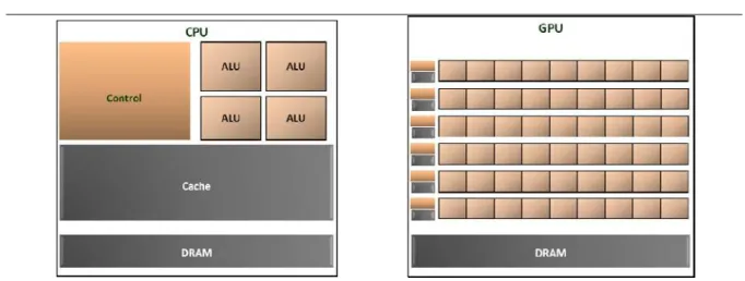
CPU and GPU design comparison

The large performance gap between multi-core CPUs and many-core GPUs is due to the difference in their fundamental design philosophy. CPUs are optimized for sequential run. As shown in Figure 2, they have a large cache memory in order to reduce memory accesses latency. In addition, they are equipped with sophisticated control logic that allows the instructions of a single thread to execute in parallel or out of their sequential order while maintaining the appearance of sequential execution. Nevertheless, the performance is not due to control or cache memory, but to the power of the Arithmetic-Logic Unit (ALU). On the other hand, GPUs are designed to have small cache memory and less complex logic unit, but a very large number of smaller cores. GPU cores are designed to execute in parallel while their execution scheduling is optimized by hardware function. The smaller GPU cache memory is covered by higher memory bandwidth to its DRAM memory due to a lighter design of this one. As a result, the high number of GPU cores is able to deliver high throughput, with lower cost and less energy.

GPUs were first developed for game industry, and thus their programmability was very limited. Even with the low programmability, successful programs were implemented for GPU execution for non-graphical applications, using the difficult graphics APIs. This was known as General Purpose programming using a Graphics Processor Unit (GP-GPU). Thus, only a very few highly skilled programmers were able to develop general purpose applications to run on the GPU. Everything changed with the release of CUDA by NVIDIA in 2007 [1]. CUDA is a C extension that allows GPU programming without passing through graphics APIs. An additional hardware was added to the GPU for this purpose. CUDA allows managing memory transfer between CPU and GPU and task scheduling for running sequential program parts on the CPU and parallel parts on the GPU. Since its apparition, many scientific and engineering applications were implemented using CUDA and high accelerations were achieved.

Even though CUDA allows GPU programming without passing through graphics API, minimum hardware knowledge is necessary for GPU programming using CUDA [2]. When an application is suitable for parallel execution, high speed-ups can be achieved over sequential execution by running it on the GPU. Usually, it is easy to obtain some speed-up for applications having data-parallelism. Nevertheless, efficient CUDA programs that achieve high speed-ups by GPU parallel

(14)

Massively Parallel Programming and Fast Computing 3

execution over sequential CPU execution require more reflection and optimization. First, it is important to efficiently handle memory operations in order to hide the long memory latency. On the other hand, it is important to have at least hundreds or thousands of concurrent threads executing in parallel in order to take advantage of the high computation throughput that could be delivered by the many GPU cores. Despite that, the acceleration that can be achieved using a GPU depends on the portion of parallel execution parts in an application. If for example % of the program execution time is spent on the part that can be parallelized, × speed-up of it will only reduce the application computation time by a factor of . . On the other hand, if the computation time of the part that can be parallelized accounts for 99 % of the sequential execution time, × speed-up of this part will reduce the application execution time by a factor of . Then it is crucial to maximize the portion of the program part that can be executed in parallel before doing an efficient CUDA implementation. For example, in magnetic resonance imaging (MRI) reconstruction, spiral scan data were replaced by Cartesian scan data for parallelization on the GPU [2]. Even though Cartesian data demands more computation on a CPU, it is more suitable for parallel execution. An optimized CUDA program using Cartesian scan allowed high speed-ups of more than × to be obtained while running MRI reconstruction on the GPU by comparison to CPU. This finally reduced scanner time from the order of hours to the order of minutes.

Another important issue is to keep low complexity and high efficiency while parallelizing methods for GPU execution. An efficient GPU code will deliver high speed-ups for GPU execution by comparison to CPU execution. Nevertheless, if the resolution scheme that is used for GPU execution demands much more computation than the original sequential scheme, the GPU acceleration will be irrelevant.

Finally, GPU programmability has helped Scientists and engineers to make breakthroughs in multiple domains due to the program accelerations that were obtained. Beginning with medical imaging, it was one of the earliest applications to take advantage of GPU computing, where for example computed tomography (CT) reconstruction has reached the level where four GPUs can do the same computation that could be done using 256 CPUs [3]. Similarly, in computational fluid dynamics, very large speedups are being achieved for Navier-Stokes models and Lattice Boltzmann methods [4, 5, 6]. GPU performances are also being useful for computational finance were for example derivative pricing algorithms are accelerated up to × [7], thus allowing more competitiveness and fast pricing results. Moreover, high speed-ups are achieved in several weather and ocean modeling applications such as numerical weather prediction [8], that enables saving in time and improvements in accuracy.

In this work, we take advantage of GPU capabilities in order to provide an extremely fast solution for computing radiation heat transfer in semi-transparent media and for computing 3D diffusion heat transfer. Work is done on the first hand in order to provide solutions methods that are highly parallelizable so they could be able to take advantage of GPU performance. Consequently, efficient GPU implementations for the solution methods are provided. On the other hand, particular effort is made in order to keep computational efficiency and low complexity of the solution methods.

(15)

4 Introduction

Simulation of Heat Transfers in High Temperature Thermal Systems

Like in many high temperature applications, heat transfers in steel reheating furnaces are mainly due to radiative exchanges between furnace objects and to heat diffusion inside its objects and more particularly the slabs to be heated. Steel reheating furnaces are then a good example of thermal systems. Thus, they are considered in this thesis for demonstrating the fast solutions that are being developed.

In general, the difficulty of computing heat diffusion in thermal systems varies depending on boundary conditions, their variation with time and the geometry of the objects where the heat diffusion has to be computed. On the other hand, the computation of radiation exchanges is usually too computationally expensive and could be done on very large size clusters having hundreds or thousands of CPUs. Moreover, its complexity increases when coupled to conduction, convection or chemical reaction. This is because the coupling necessitates finer mesh to be applied for computing radiation heat transfer in order to provide accurate boundary conditions for other heat transfer modes.

Moreover, thermal systems control requires real time simulations, thus demanding not only high computational throughput but also more importantly fast solutions that allow the computations to be achieved in real time.

In the following some applications are considered in order to illustrate the complexity of the computation that arises primarily for computing radiation heat exchanges and then for computing heat diffusion.

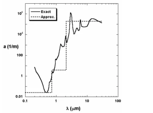
Consider first the analysis of a steam explosion in a nuclear reactor obtained by the in the mixture of hot molten nuclear fuel at 3000 K with water (figure 4). Understanding the premixing process in this reaction and knowing the water quantity in the reactor is the key for controlling the boiler process and the reactor safety. The presence of high temperatures due to the nuclear fuel implies that water temperature profile in the reactor to be highly varying. Thus, due to the high variation of the absorption coefficient of water with temperature (figure 5), radiative exchanges have to account for the highly non-gray and varying absorption coefficient in the reaction. Besides, the rapidity of the reaction implies very small computation time steps for the computation.

(16)

Simulation of Heat Transfers in High Temperature Thermal Systems 5

Figure 5: The 3-band approximation of water absorption coefficient used in the premixing

calculation.

Besides its importance in heat transfer, radiation is the basis for illumination, which is very challenging for the video industry. Every advance in illumination techniques provides more options in games and imaging as well as it provides better and more realistic effects and images. In video games, illumination has to be computed in real-time with every change of positions and light sources. Radiation exchanges have then to be computed many times in one second in order to provide real illumination effects in the video image.

In addition to mathematical complexity, recall to the difficulty of computing radiative exchanges in inverse problems as for determining radiative properties for surfaces or volumes. Radiative properties depend on temperature, surface roughness and degree of polish and it depends on mixture proportions in gases. In inverse problems, the computation of radiative exchanges has to be repeated with different radiative emissivities and absorptivities in order to reach the input temperature profiles, which indicates that accurate radiative properties have been found. Actually, in addition to that many radiative properties have to be accounted for in one single application, thus too many repetitions of the computation are required.

Finally, consider the application case of this thesis that is steel reheating furnaces. The inline control for an industrial furnace consists of hundreds of thousands of lines of code. Nevertheless, the only too time consuming part in such programs is the computation of the heat transfer in the furnace. Due to high temperatures, the heat transfers inside a steel reheating furnace are dominated by radiation. Convection effects could be neglected. The computation of heat transfer in a steel reheating furnace consists then of computing radiation exchanges between the objects in the furnace and coupling radiation to heat diffusion inside the furnace objects, the most important being the heat diffusion inside the slabs. Computing the 3D heat transfers in the whole furnace and knowing the 3D temperature profiles of the slabs at each position of the furnace allows higher level

(17)

6 Introduction

of furnace control. The result of that will be better heat quality and better energy efficiency. In contrast, the systems that are available to this date allow only 1D or 2D slab temperature profiles to be computed, while radiation exchanges are usually computed in advance with very large mesh size. Thus, the values of radiative exchange factors lack in precision and the mesh sizes are very large in order to provide precise boundary conditions for computing heat diffusion in the slabs. In this work, we provide a fast solution for computing radiation heat transfer in 3D semi-transparent media based on the Multiple Absorption Coefficient Zonal Method (MACZM). In addition, a fast solution of heat diffusion is given based on an optimized GPU parallelization of the finite difference Locally One Dimensional (LOD) split method. As a result, the whole radiation exchanges in a steel reheating furnace will be able to be solved in about a second with a high precision mesh size. This is fast enough in order to allow dynamic simulation of the radiation exchanges for the inline control on the first hand and on the second hand, it provides precise boundary conditions for computing the heat diffusion in the slabs or the other furnace components. Besides, the given solution for the heat diffusion allows a high precision and very fast computation of the 3D heat diffusion in the slabs. As for example, given a time step of one second it allows to completely compute the 3D heat diffusion in a slab for the five hours time that it stays in the furnace, in less than a minute.

Manuscript Overview

Chapters 1 through 3 are dedicated for the computation of radiative exchange factors. Chapter 1 presents a numerical and experimental validation of the multiple absorption coefficient zonal method (MACZM) for computing direct radiative exchange factors in 3D inhomogeneous non-gray media. It first represents an overview of MACZM as well as the definition of Mean Beam Lengths (MBLs) that allow the computation to be done using artificial neural networks (ANNs). Then it describes the flux planes method for computing direct radiative exchange factors. Flux planes method is then used for validating MACZM for the computation of direct exchange factors between volume and surface elements. At the end of this chapter, MACZM accuracy is validated experimentally and by comparison to the flux planes method over a steel reheating test furnace. Finally, the advantage of MACZM in computation time is highlighted.

Chapter 2 covers efficient CPU and GPU implementations of the multiple absorption coefficient zonal method. In the first part of chapter 2, the algorithm corresponding to MACZM is described. Grid generation and connectivity control relative to space discretization and the method computations are discussed. Then, three efficient line discretization algorithms with linear complexity property are adapted for MACZM algorithm and compared and the best of them is kept for the implementation. In the second part of chapter 2, an efficient GPU parallel implementation of the MACZM using CUDA is represented. In this issue, GPU memory handling and efficient implementation of the different parts of the MACZM algorithm are presented. A very brief introduction to CUDA is given in that part. The reader who is totally unfamiliar with CUDA should refer first to Appendix A for better understanding of how CUDA works or skip this part directly to the application part. The last part of the chapter covers a multi-grid approach for MACZM in order to avoid unnecessary computations. The steel reheating furnace application is considered in order to describe the multi-grid approach.

(18)

REFERENCES 7

Chapter 3 covers the computation of total radiative exchange factors. Even though this chapter completes the previous two chapters, there is no continuity between this chapter and the previous ones. In chapter 3, the plating algorithm for computing total exchange factors from direct exchange factors is first reviewed. A Non-Recursive Plating Algorithm (NRPA) is then formulated by identification to the plating algorithm in order to avoid recursion in computations. The NRPA is then written in matrix form that consists mainly of a matrix multiplication operation. Reduction in computational complexity for the NRPA is then achieved based on low complexity matrix multiplication algorithms. Finally, CPU and GPU implementations of the NRPA are then given based on linear algebra libraries. Besides, Multi-core CPU parallelization and GPU parallelization of the plating algorithm are presented at the end of the chapter. Sequential and parallel PA and NRPA computation time comparison is then given.

Chapter 4 is devoted for the 3D solution of the heat diffusion in slabs. First, it presents a fast review of finite difference approximation and discretization. Explicit, implicit and Crank-Nicolson schemes are reviewed. Then a review of the finite difference split methods that have less computation complexity is given. Since the split methods require the solution of tridiagonal system of linear equations, efficient sequential and parallel tri-diagonal system solvers are reviewed. A highly parallel parallelization scheme for GPU execution of the Locally One Dimensional (LOD) split method is then presented. In addition, stencil parallelization scheme is reviewed. Finally, an optimal hybrid parallelization scheme and solver strategy for running LOD method on the GPU that delivers high speed-ups is presented. The chapter ends with a simple analytical verification of the split methods that were reviewed complemented by an accuracy analysis on the influence of time and space discretization steps.

Finally, chapter 5 demonstrates an efficient thermal solution of a steel reheating furnace based on the methods and algorithms presented in the previous chapters. In this chapter, an efficient 3D numerical model for solving radiation and conduction in a steel heat furnace is first presented. Then an approach for 3D thermal analysis of the furnace is discussed. In the analysis, an approximate analytical solution is given for taking into account the cooling effect of furnace rails. The 3D temperature profiles of the slabs is then given at any time of the heating process, which makes it possible to determine the low temperature zones on the slabs, called black points. Finally, an appropriate configuration of the rails position in the furnace that results in better temperature uniformity in the slabs is determined.

REFERENCES

1. NVIDIA. CUDA Technology; http://www.nvidia.com/CUDA, 2007.

2. D. B. Kirk, W. W. Hwu, Programming Massively Parallel Processors a Hands on Approach, Elsevier inc., 2010

3. H. Scherl, B. Keck, M. Kowarschik, J. Hornegger, Fast GPU-Based CT Reconstruction using the Common Unified Device Architecture (CUDA), NSS 07 IEEE, Nuclear Science Symposium, 2007

(19)

8 Introduction

4. J. M. Cohen, M. J. Molemaker, A Fast Double Precision CFD Code using CUDA, In 21st International Conference on Parallel Computational Fluid Dynamics, 2009.

5. Y. Zhao, Lattice Boltzmann based solver on the GPU, International Journal of Computer Graphics, vol. 24 (5), pp. 323-333, 2009

6. G. Stanvech, D. Juba, W. Dorland, and A. Varshney, Using Graphics Processors for High-Performance Computation and Visualization of Plasma Turbulence, Journal of Computing in Science and Engineering, vol. 11 (2), pp. 52-59, 2009.

7. OnEye High Performance Computing, Using GPU to Compute Options and Derivatives, OnEye Pty Ltd, Sydney, Australia, 2008.

8. J. Michalakes, GPU Acceleration of Numerical Weather Prediction, International Symposium on Parallel and Distributed Processing, IEEE, 2008

(20)

CHAPTER

Direct Exchange Factors

Computation Method

1

CHAPTER CONTENTS

1.1 Introduction ... Erreur ! Signet non défini. 1.2 Multiple Absorption Coefficient Zonal Method (MACZM) ... Erreur ! Signet non défini. 1.3 Modray Tool Description ... Erreur ! Signet non défini. 1.4 Elementary Operations Validation ... Erreur ! Signet non défini. 1.5 Test Case Description ... Erreur ! Signet non défini. 1.6 Calculation of Radiative Exchange Factors ... Erreur ! Signet non défini. 1.7 Experimental Validation ... Erreur ! Signet non défini. 1.8 Conclusions ... Erreur ! Signet non défini. References ... Erreur ! Signet non défini.

(21)

10 Chapter 1 Direct Exchange Factors Computation Method

EXPERIMENTAL VALIDATION OF THE MULTIPLE ABSORPTION

COEFFICIENT ZONAL METHOD (MACZM) IN A DYNAMIC MODELING

OF A STEEL REHEATING FURNACE

Boutros Ghannam

11

, Maroun Nemer

1

, Khalil El Khoury

2

, and Walter Yuen

3

1

Mines ParisTech, CEP – Center for Energy and Process Studies 60, boulevard Saint-Michel – F – 75272 Paris Cedex 06

2_{Lebanese University, Roumieh, Lebanon}

3

University of California Santa Barbara, Santa Barbara, CA 93106 United States

Abstract -

In this work, the multiple absorption coefficient zonal method (MACZM) is being implemented and validated numerically. The method is demonstrated to be highly suitable for the analysis of radiative heat transfer in multi-dimensional inhomogeneous non-grey media. A uniform rectangular fine grid is considered and small CPU time is achieved. This makes the method of great interest for transient applications. The validity of the method is demonstrated in two steps. First, cases with simple geometry are considered and results are compared to results generated by direct numerical integration. Results are also generated by MODRAY, which is a source project based on an original method called the flux-planes approximation, and are shown to be equally accurate. Second, the case of a steel reheating furnace is considered. In a previous work, the furnace heat balance and temperature profiles were simulated using a finite difference computation approach and radiative exchange factors generated by MODRAY. Experiments were performed and results generated by the model were found to be in good agreement with experimental data. The radiative exchange factors are now recalculated with MACZM. They are shown to be very close to those generated by MODRAY. The comparison of the two methods clearly shows that MACZM is much faster for the calculation of the volume-volume radiative exchange factors on a uniform rectangular grid.

(22)

CHAPTER

Implementation and

Parallelization of MACZM

2

CHAPTER CONTENTS

2.1 Introduction ... Erreur ! Signet non défini. 2.2 Multiple Absorption Coefficient Zonal Method (Maczm) and Algorithm Erreur ! Signet non

défini.

2.3 Grid Generation And Representation of the Objects in The Discrete Space ... Erreur ! Signet

non défini.

2.4 Mean Absorption Coefficient Computation by Ray Tracing ... Erreur ! Signet non défini. 2.5 Artificial Neural Network and GEF Superposition ... Erreur ! Signet non défini. 2.6 Gpu Cuda Programming Model Overview ... Erreur ! Signet non défini. 2.7 Parallel Implementation of MACZM in CUDA ... Erreur ! Signet non défini. 2.8 Application: Simulation of a Steel Reheating Furnace ... Erreur ! Signet non défini. 2.9 Conclusions ... Erreur ! Signet non défini. References ... Erreur ! Signet non défini.

(23)

32 Chapter 2 Implementation and Parallelization of MACZM

AN EFFICIENT CPU - GPU IMPLEMENTATION OF THE MULTIPLE

ABSORPTION COEFFICIENT ZONAL METHOD (MACZM)

Boutros Ghannam

12

, Maroun Nemer

1

, Khalil El Khoury

1

, and Walter Yuen

2

1

MINES ParisTech, CEP – Center for Energy and Processes 60, boulevard Saint-Michel – F – 75272 Paris Cedex 06 2

University of California Santa Barbara, Santa Barbara, CA 93106 United States

Abstract -

The multiple absorption coefficient zonal method (MACZM) is an efficient radiative heat transfer modeling method in non-isothermal inhomogeneous media. The method is of high interest for dynamic applications because of its ability to asses semi-transparent radiative heat transfer in very short computation time. In this work, an efficient algorithm for MACZM is implemented. A connectivity control study is presented for taking into account the connectivity considerations required by the method. An identified ray traversal algorithm corresponding to part of the MACZM implementation is then selected among three different approaches presented in the paper, based on the famous ray traversal algorithms the 6-tripod line algorithm and the 6-parametric line algorithm. On another hand, the MACZM is highly parallel and is implemented in CUDA, a parallel computing architecture that enables an easy use of the powerful graphics processing unit (GPU). An efficient implementation is discussed consisting of an optimal solution for exploiting the method parallelism (threading) and the use of the memory resources available on the GPU. Speed-ups going from 300 to 600 times are achieved, using a NVIDIA Tesla C 1060 GPU and an Intel Xeon CPU E5507 at 2.27 GHz. Radiative heat transfer is then simulated in a steel reheating furnace using the optimized GPU implementation. The computation time is further reduced using a multi-grid approach.

(24)

CHAPTER

Total Exchange Factors

Computation by NRPA

3

CHAPTER CONTENTS

3.1 Introduction ... Erreur ! Signet non défini. 3.2 Plating Algorithm Mathematical Formulation ... Erreur ! Signet non défini. 3.3 Formulation of the Non-Recursive Plating Algorithm (NRPA) ... Erreur ! Signet non défini. 3.4 Matrix Form of the NRPA ... Erreur ! Signet non défini. 3.5 Reducing The Computational Complexity of the NRPA Via Matrix Multiplication .. Erreur !

Signet non défini.

3.6 Testing The Error of Non-Recursive Plating Algorithm ... Erreur ! Signet non défini. 3.7 Implementation And Computation Time Comparison of the PA And The NRPA ... Erreur !

3.8 Conclusions ... Erreur ! Signet non défini. References ... Erreur ! Signet non défini.

(25)

58 Chapter 3 Total Exchange Factors Computation by NRPA

THE NON-RECURSIVE PLATING ALGORITHM (NRPA) FOR COMPUTING

TOTAL RADIATIVE EXCHANGE FACTORS IN ENCLOSURES

Boutros Ghannam

13

, Maroun Nemer

1

, Khalil El Khoury

1

MINES ParisTech, CEP – Center for Energy and Processes

60, boulevard Saint-Michel – F – 75272 Paris Cedex 06

Abstract

Many numerical methods for computing radiation exchange in enclosures are based on the computation of direct exchange areas (DEAs) and total exchange areas (TEAs). Excessively long computation times can be associated to TEAs computation. Among the most performing methods, the plating algorithm (PA) computes TEAs from DEAs based on a set of simple recursive equations. An efficient CPU and GPU parallelization of the PA are represented. Nevertheless, PA computation complexity is . A novel formulation, the non-recursive plating algorithm (NRPA) is introduced. It allows the computation of TEAs with one single non-recursive step. Its equations are formulated by identification to the PA equations giving TEAs from DEAs, requiring one simple assumption. The NRPA is then written in matrix form as mainly a square matrix multiplication operation. Based on advancement in matrix multiplication computation, the NRPA complexity is proven to be . for the number of multiplications. CPU and GPU NRPA are implemented based on the optimized linear algebra library BLAS for CPU and cuBLAS for GPU CUDA programs. NRPA is found to highly outperform PA in both CPU and GPU computation times. Finally, a test enclosure is considered in order to validate the accuracy of the NRPA by comparison to the PA.

(26)

CHAPTER

3D Heat Diffusion

computation

4

CHAPTER CONTENTS

4.1 Introduction ... Erreur ! Signet non défini. 4.2 Discrete Approximation of The 3d Heat Diffusion Equation by Finite Differences ... Erreur !

4.3 Finite Differences Split Methods Applied to the 3d Heat Diffusion PDE .. Erreur ! Signet non

défini.

4.4 Highly Efficient Tridiagonal Linear System Solvers ... Erreur ! Signet non défini. 4.5 Gpu Cuda Programming Model Overview ... Erreur ! Signet non défini. 4.6 Parallelization of the Split Methods And Implementation In CUDA ... Erreur ! Signet non

défini.

4.7 Highly Efficient GPU Implementation of the LOD Method Using Optimal Solvers and Parallelization Schemes ... Erreur ! Signet non défini. 4.8 Analytical Validation of the Split Methods ... 111 4.9 Analysis by Example of the Accuracy of the Split Methods in Order to Time and Space Mesh Size ... 113 4.10 Conclusions ... Erreur ! Signet non défini. References ... Erreur ! Signet non défini.

(27)

86 0 3D Heat Diffusion computation

A FAST SOLUTION OF THE 3D HEAT DIFFUSION EQUATION BY FINITE

DIFFERENCE SPLIT METHODS AND AN EFFICIENT GPU

PARALLELIZATION

Boutros Ghannam

14

, Maroun Nemer

1

Mines ParisTech, CEP – Center for Energy and Processes

60, boulevard Saint-Michel – F – 75272 Paris Cedex 06

Abstract

In this paper an optimal and efficient numerical solution of the 3D heat diffusion Equation on GPUs is presented. The solution is the result of the optimized combination between finite difference discretization scheme, parallelization schemes in CUDA, and appropriate tridiagonal matrix solvers. Finite difference split methods are used for their low computational complexity and parallelization property. At the first hand, a new parallelization scheme is applied for the solution of the Locally One Dimensional (LOD) method. The scheme is shown to give high accelerations going up to 60 times by comparison to CPU time, beginning from small grid size. On the other hand, Thomas algorithm for the solution of linear tridiagonal systems is used for the first time, together with a stencil parallelization. It is shown to deliver higher performance by comparison to the first scheme with large grid size, with up 250 times acceleration by comparison to CPU time. Finally, a combined alternating parallel scheme solution is discussed, allowing an optimal performance to be achieved even for small grid size.

(28)

ANALYTICAL VALIDATION OF THE SPLIT METHODS

111

4.8 ANALYTICAL VALIDATION OF THE SPLIT METHODS

4.8.1 Setting the problem

A cube of dimensions × × is

considered for the validation (Figure 14). The cube is at initial temperature = and exchanges heat by convection to a heat source

of temperature = . A constant

convection heat exchange coefficient ℎ = . is considered on all sides of the cube. Because of an analytical solution, the physical properties of the cube are considered to be constant during the whole heating time,

giving a conductivity = . , a

heat capacity = . , and density

= . .

4.8.2 Analytical solution

The analytical solution for the considered three-dimensional case is the product of three one- dimensional analytical solutions of the transient heat conduction in a plain wall (Figure 15).

The governing PDE for the one-dimensional heat diffusion is as follows:

= Where = / is the diffusivity of the material.

Figure 14: Cube submitted to convection heat

(29)

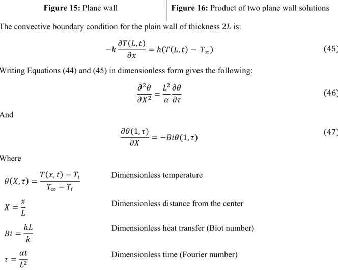
Figure 15: Plane wall Figure 16: Product of two plane wall solutions

The convective boundary condition for the plain wall of thickness is:

− , = ℎ , −

Writing Equations (44) and (45) in dimensionless form gives the following:

= And , = − , Where , = , −₋ Dimensionless temperature

= Dimensionless distance from the center

=ℎ Dimensionless heat transfer (Biot number)

= Dimensionless time (Fourier number)

The analytical solution for the temperature profile in the plain wall is given as a function of the dimensionless variables as:

, = sin_sin cos ⁄

Where values are the solution of tan = .

This solution can be approximated by its first term for > . with an error that is less than 2%. Thus if we consider the temperature at the center plane of the plain wall, it is given by:

, = sin

sin For > . .

Finally, the analytical solution for the temperature at the center point of the cube is the product of the solutions of three identical solutions of the temperature at the center plane of a plain wall (Figure 16). The solution is then given by:

, = , × , × ,

(30)

, = ₋, − = . .

The analytical solution is given in Figure 17 for > , in order to guarantee that > . .

Comparison to numerical solution

The temperature is computed by all the split methods using grid size × × and a time step of . The resulting solution is presented in Figure 17 for > in order to compare it to the analytical solution. As it could be observed on Figure 17, all numerical solutions are very close to the analytical solution. The error of the numerical solutions is always less than . % by comparison to the analytical solution, which demonstrates the validity of the solution that were given by the split methods.

Figure 17: Comparison of numerical solutions to the analytic solution

4.9 ANALYSIS BY EXAMPLE OF THE ACCURACY OF THE

SPLIT METHODS AS A FUNCTION OF TIME AND SPACE

MESH SIZE

4.9.1 Numerical simulation

Consider a steel slab of size

. × . × . . The slabs

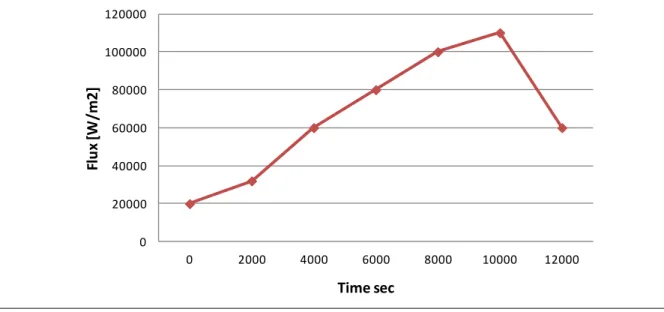
lays on two supports as presented in Figure 18. The slab is heated by the surface flux profile of Figure 19. The heat flux is supposed to be null at the contact with the supports. The slab temperature is computed separately by the different split methods over a period of 15000s. The physical properties in the slab vary with

0 200 400 600 800 1000 1200 1400 1600 Analytic LOD Pe-Ra Do-Gu

Temperature variation at the center of the cube

T (k)

t (s)

(31)

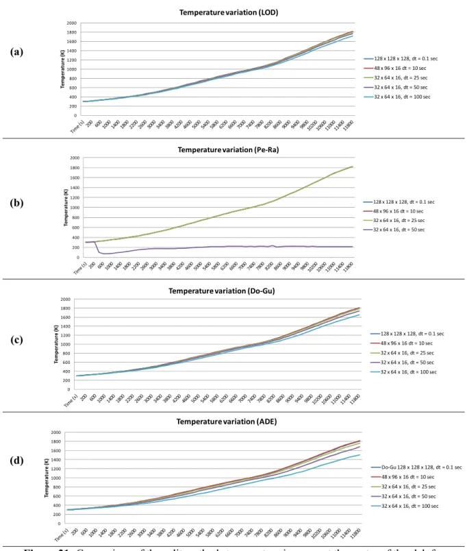
the temperature during the simulation. A very fine meshing is first considered consisting of × × space mesh and a time step of . second. The resulting variation of the temperature at the center of the slab and at the quarter of the height over the support that were obtained by the different split methods are presented in Figures 20.a and 20.b. The slab is then simulated by each method using different space and time steps. The results of the simulations at the center of the slab are presented in Figure 21 (21.a-21.e).

Figure 19: Heating flux as a function of time.

4.9.2 Comparison and analysis

In Figure 20, for a fine meshing, all methods give the same temperature profile. This was expected and it validates the consistency and convergence property of the different methods. On the other hand, Figure 21 demonstrates the stability and the accuracy of each method. As it could be observed, the LOD method (Figure 21.a) and the Douglas-Gunn ADI method (Figure 21.b) give the

0 20000 40000 60000 80000 100000 120000 0 2000 4000 6000 8000 10000 12000 Fl u x [ W /m 2 ]

Flux [W/m2]

Time sec

Figure 20: Temperature increase at the center of the slab as a function of time. 0 200 400 600 800 1000 1200 1400 1600 1800 2000 T e mp er a tu re ( K )

Temperature variation at the center

LOD Pe-Ra Do-Gu ADE (48 96 16)

(32)

most accurate results with lower space and time mesh. This is because they are unconditionally stable and second order accurate in time and space. As for the ADE method (Figure 21.c), it is less precise when lower space and time steps are considered, even though it is still stable with large time steps. On the other hand, the Peaceman-Rachford ADI method (Figure 21.d) is first order accurate in time, thus its error becomes larger when larger time step is considered and it becomes unstable when for very large time steps.

(a)

(b)

(c)

(d)

Figure 21: Comparison of the split methods temperature increase at the center of the slab for

different space and time mesh.

0 200 400 600 800 1000 1200 1400 1600 1800 2000 Te m p e ra tu re ( K )

Temperature variation (LOD)

128 x 128 x 128, dt = 0.1 sec 48 x 96 x 16 dt = 10 sec 32 x 64 x 16, dt = 25 sec 32 x 64 x 16, dt = 50 sec 32 x 64 x 16, dt = 100 sec 0 200 400 600 800 1000 1200 1400 1600 1800 2000 Te m p e ra tu re ( K )

Temperature variation (Pe-Ra)

128 x 128 x 128, dt = 0.1 sec 48 x 96 x 16 dt = 10 sec 32 x 64 x 16, dt = 25 sec 32 x 64 x 16, dt = 50 sec 0 200 400 600 800 1000 1200 1400 1600 1800 2000 Te m p er a tu re ( K )

Temperature variation (Do-Gu)

128 x 128 x 128, dt = 0.1 sec 48 x 96 x 16 dt = 10 sec 32 x 64 x 16, dt = 25 sec 32 x 64 x 16, dt = 50 sec 32 x 64 x 16, dt = 100 sec 0 200 400 600 800 1000 1200 1400 1600 1800 2000 Tem p er a tu re ( K )

Temperature variation (ADE)

Do-Gu 128 x 128 x 128, dt = 0.1 sec 48 x 96 x 16 dt = 10 sec 32 x 64 x 16, dt = 25 sec 32 x 64 x 16, dt = 50 sec 32 x 64 x 16, dt = 100 sec

(33)

(34)

CHAPTER

CHAPTER CONTENTS

5.1 Introduction ... 117 5.2 3d Numerical Computation Model for a Steel Reheating Furnace And Performance Evaluation ... 120 5.3 Application: Thermal Analysis of a Steel Reheating Furnace ... 125 5.4 Optimization of Rails Positions and Heating Temperature Profiles ... 127 5.5 Conclusions and Future Work ... 131

NOMENCLATURE

Surface area

Thermal conductivity

Transfer factor

Zone number

Number of furnace patitions

Heat flux

Temperature

Greek symbols

Stefan-Boltzmann constant

5.1 INTRODUCTION

Applications where the radiative heat exchange is dominant are very challenging. Steel reheating furnaces are a good example of application where the radiative heat exchange is dominant, because of the high operating temperatures. A steel reheating furnace is filled with non-homogeneous media from combustion gases. Steel slabs circulate in the furnace in order to be reheated to temperatures around ℃. After the slabs are heated, they are submitted to a post treatment process as rolling for example. In order to achieve a good quality of the post treatment process, the temperature profile of the slabs leaving the furnace must correspond to a specific set point. In the case of rolling for example, a uniform temperature profile is needed. In addition, the heating profile of the slabs is

3D Ultra-Fast Simulation

of Steel Reheating

Furnace, Opening for

Inline Control

(35)

120 3D Ultra-Fast Simulation of Steel Reheating Furnace, Opening for Inline Control

also object to a set point in order guarantee better energy efficiency on the first hand and achieve the desired temperature profile in the slabs at the end of the furnace on the second hand.

Heating temperature profile set point and final temperature profile of the slabs can be achieved using inline controllers. Because of the high operating temperatures and the slabs movement in the furnace, it is impossible to continuously measure the slabs temperature in the furnace. Thus, it is necessary to numerically compute the temperature profiles in the slabs and the rest of the furnace. Moreover, with numerical computation it is possible to make computations for the next minutes or hours of heating before reaching them, which is crucial in order to build efficient inline control strategies.

In contrast, the numerical solvers that were developed earlier lack in speed and precision. They usually are too slow in order to compute inline temperature profiles in the furnace. In consequence, simplifications are usually made, considering of computing the heat diffusion in the slabs in 1D or 2D and setting a low-resolution mesh for computing radiative heat exchanges. On the other hand, the temperature profiles for the forthcoming operating time of the furnace are only predicted in order to be used for the inline control, instead of being precisely computed.

In this chapter, first a detailed numerical solver for the heat exchanges in the furnace is presented based on the methods developed in the previous chapters. The multi-grid approach is used for computing the direct exchange factors. In addition, computation of the insignificant direct exchange factors is eliminated. A zone approach is then introduced for applying the NRPA in order to make the computation of the total exchange factors as fast as the computation of the direct exchange factors. The radiation is then coupled to heat diffusion, which is computed using the efficient LOD scheme presented in chapter 4. As a result, a high precision 3D numerical solver is set and very fast computation time is achieved, that allows inline dynamic computation and computation of the forthcoming functioning time.

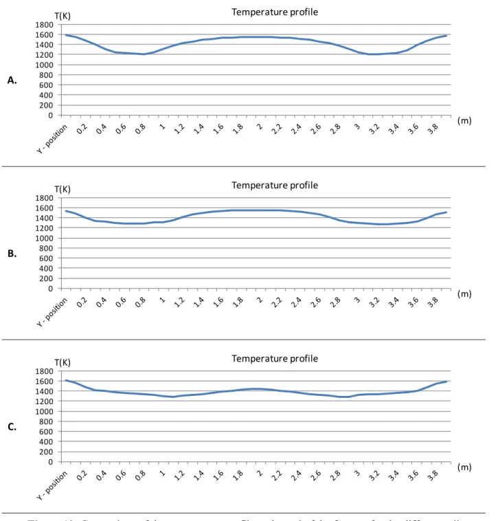
A thermal model for solving the heat exchanges in the furnace is then presented. Using this model, an analysis of black points is given based on the configuration of the positions of the rails. Black points are the zones of the slab where the temperature is lower due to the cooling by the contact with the supporting rails. On the other hand, a wall temperature profile is determined that allows a desired delayed heating temperature profile to be achieved in the slabs.

5.2 3D NUMERICAL COMPUTATION MODEL FOR A STEEL

REHEATING FURNACE AND PERFORMANCE

EVALUATION

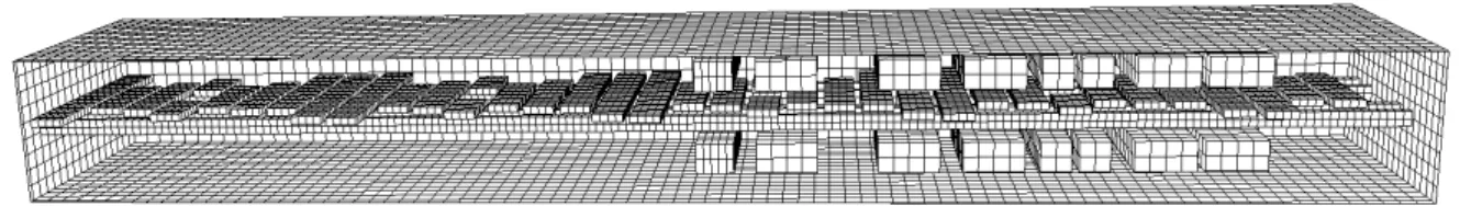
Consider the steel reheating furnace of chapter 2.8. The internal dimensions of the furnace are . × . × . . Figure 1 shows the elements inside the furnace. The furnace can hold on average slabs of steel laid on four rails. The slabs of steel have different lengths but they all have a height of . and a width of . (Figure 1).

(36)

5.2 3D NUMERICAL COMPUTATION MODEL FOR A STEEL REHEATING FURNACE AND PERFORMANCE EVALUATION

121

An average distance of . is supposed to be separating the steel slabs over the length of the furnace. The rails are assumed to have a rectangular section of size . × . . The first part of the furnace is a preheating zone with no burners where the slabs receive heat flux from the hot gazes coming from the heating zone.

The heating zone is equipped by regenerative burners that are symmetrically positioned in the upper and lower zones of the furnace. All burners are identical and the combustion volumes are assumed to be rectangular with dimensions . × × . . An emissivity of 0.9 is assumed for the furnace walls. The slabs are assumed to have an emissivity of 0.8 and the rails an emissivity of 0.75. The volume of the furnace is filled with combustion gases that are supposed to be acting as gray-diffusive and non-scattering with an absorptivity of 0.5 .

5.2.1 Computation of the direct radiative exchange factors

The direct radiative exchange factors are computed by the Multiple Absorption Coefficient Zonal Mehtod using the multi-grid approach presented in Chapter 2.8.5. The multi-grid approach implies that each category of exchange factors is computed using an appropriate mesh size in order to guarantee a good accuracy and to avoid any unnecessary calculation time. A mesh size of 40 (0.15 Mvoxels) is applied to the furnace in order to compute the direct exchange factors between the burners and the direct exchange factors between the furnace walls. Direct exchange factors between walls and steel slabs, rails and burners as well as between burners and walls are computed using a mesh size of 20 (1.2 Mvoxels). At last, a mesh size of size 10 (over 9 voxels) is considered in order to compute direct exchange factors between the slabs themselves and between slabs and rails. A larger mesh being less accurate for computing the former exchange factors because of the dimensions and the relative position of the slabs to the rails and the slabs between them. At this level, a CPU computation time of 1200 seconds is achieved for one single of the direct exchange factors in the furnace, while GPU execution is about 320 times faster with a computation time of 3.6 seconds, using an Intel Xeon CPU E5507 at 2.27 GHz and a NVIDIA Tesla GPU C 1060.

(37)

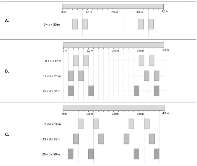
At the end, the computed direct exchange factors are associated together in order to give for each object the highest dimension of mesh that were applied to it during the computations. Figure 2 shows the final meshing of the furnace. The final mesh size is 20 for steel slabs and the rails while a mesh size of 40 is given to the burners, the furnace volume and walls.

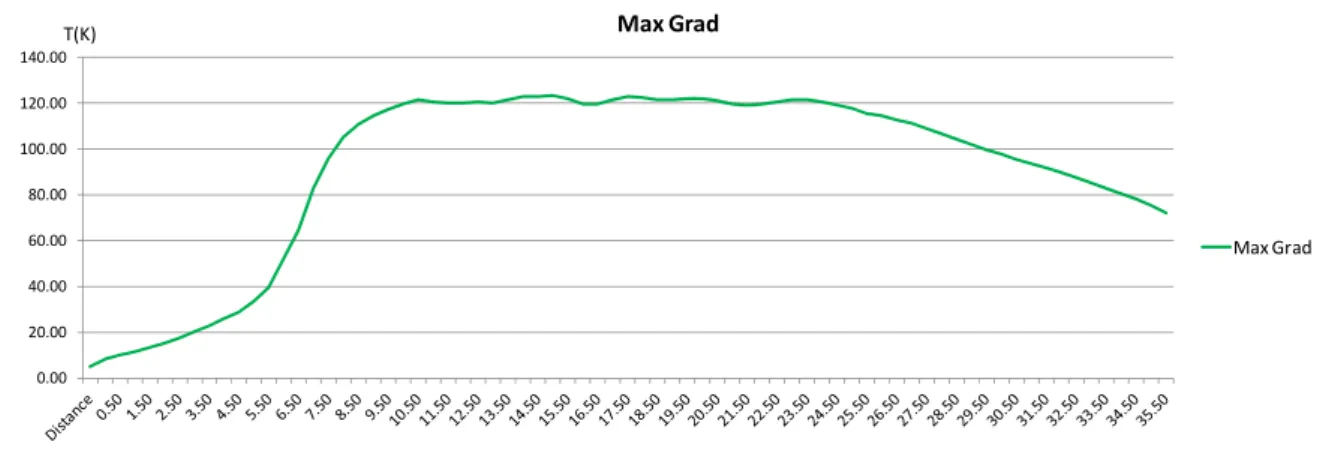
Further saving in computation time is done by eliminating the computation of insignificant direct exchange factors. Because of the low ratio of the width and height of the furnace to its length, the direct exchange radiation leaving a surface element at for example the middle of the furnace is absorbed long before it reaches the beginning or the end of the furnace (Figure 3).

The limiting distance from which the radiative exchange is negligible is determined dynamically while computing the radiative exchange factors. Beginning the computation from neighboor vertical planes and going up to distant planes, the computation is stopped when the summation of the direct exchange factors is at 99% of its value. As a result, a CPU computation time of 180 seconds and a GPU time of less than a second are achieved.

Figure 3: Limiting the computation of direct exchange factors over the length of the furnace

5.2.2 Computation of the total radiative exchange factors

Given the emissivities of the furnace surfaces and the direct exchange factors between all the surface elements, the total exchange factors are computed using the plating algorithm. The total number of surface elements in the furnace after the multi-grid approach is applied is 14660. Applying the plating algorithm directly to the furnace with this number of surfaces elements would necessitate about two hours CPU computation time, which is too slow by comparison to the computation of the direct exchange factors.

(38)

5.2 3D NUMERICAL COMPUTATION MODEL FOR A STEEL REHEATING FURNACE AND PERFORMANCE EVALUATION

123

On the other hand, applying the NRPA to compute the total exchange factors requires a GPU computation time of 9 seconds at order 2 and 17 seconds at order 3. The corresponding weighted average errors by comparison to the plating algorithm being 3% and 1 % respectively for order 2 and order 3 NRPA respectively.

The NRPA computation time is still an order of magnitude higher than the computation time of direct exchange areas. Thus, it is still the limiting factor for the computation time. As a solution, the total exchange factors could be approximated by dividing the furnace to a number of computation zones. Applying the NRPA to zones with lower number of surface elements results in faster computation time since the NRPA is of order . . The zone computation is shown in figure 4.

The furnace is first divided into zones in the length direction. The total exchange areas of a zone are then computed by taking into account the plating of surface elements of the zones − , and + . Using N=10, a computation time of 0.75 seconds is achieved by the order 3 NRPA with an additional error varying between 1 and 2 % over the computed total exchange areas. In this case, the NRPA is applied to systems with lower number of surfaces .

5.2.3 Computation of temperature profiles in the slabs

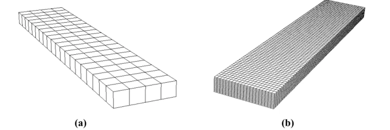
A slab temperature profile is given by computing the heat diffusion in the slab given the adequate boundary conditions. The heat diffusion in the slabs is computed by the LOD method (Chapter 4.3.1). A fine mesh is applied to the slabs for the computation. Neglecting convection, the boundary conditions on the slabs are flux boundary conditions due to the radiation between the slab surfaces and other surfaces and volumes in the furnace and to the heat conduction to the rails. Even though the mesh considered for computing radiative exchange factors is fine and sufficiently precise, the corresponding mesh size still is larger than the mesh that is applied for computing heat diffusion by finite differences (Figure 5). Consequently, the computed radiative heat flux is projected on the diffusion mesh in order to give the flux boundary condition. If more than a radiative computation mesh intersect on a diffusion computation mesh area, the corresponding radiative heat flux is computed as the average of the intersecting radiative fluxes, each of them being weighted by the proportion of its corresponding surface area proportion on the diffusion mesh.

A central first order finite difference approximation of the flux boundary conditions is considered for applying the LOD method in order to guarantee that the result is still second order accurate.

(39)

The computation is done using the highly efficient GPU implementation given in chapter 4.7. It achieves a very fast computation time. For example, using a grid of × × meshes, allows achieving a computation time lower than 1/3000 seconds by time step. A highly accurate 3D temperature profile in all the slabs is finally obtained.

5.2.4 Dynamic simulation and performance evaluation

The slabs are moving at a speed of . . Maximum precision for the simulations is obtained if the computation of the radiative exchange factors is done for the smaller possible distance step in the slab moving direction. From the previous section, the largest mesh size used for computing direct exchange factors between a surface element on a slab and any other surface element in the furnace is . This implies that the minimum distance step that could be considered for computing radiative exchange factors is . The radiative exchange factors should then be computed for a distance step of or equally a time step of seconds. The computation time that is needed to achieve the computation of radiative exchange factors relative to one time step is about . seconds (NVIDIA Tesla GPU C 1060). A time step of seconds is then large enough to allow real-time dynamic simulation of the furnace since it is much higher than

. seconds.

The time step for radiative exchange factors computation is then 80 seconds, which implies that heat diffusion will have to be computed using a time step that is smaller than 80 seconds. Even if the radiative exchange factors are constant over a 80 second time period; the radiative heat flux on the slabs could be varying during this period, since the temperatures of the slab and the furnace are varying continuously.

A grid of × × meshes for the computation of heat diffusion in the slabs will keep a good precision and a fast computation time. From the diffusion computing section, the computation time corresponding to this mesh is / seconds by slab and by time step. Then computing the diffusion in all the slabs of the furnace will require . seconds, defining then the minimum time step for computing heat diffusion in the real-time dynamic simulation. Obviously, much higher time steps would be considered for the heat diffusion computation, since the accuracy of the results will not be significantly affected.

(a) (b)

Figure 5: Coupling radiation and diffusion (a) Slab mesh for computing radiation exchange factors