HAL Id: pastel-00002803
https://pastel.archives-ouvertes.fr/pastel-00002803
Submitted on 28 Sep 2007
HAL is a multi-disciplinary open access archive for the deposit and dissemination of sci-entific research documents, whether they are pub-lished or not. The documents may come from teaching and research institutions in France or abroad, or from public or private research centers.
L’archive ouverte pluridisciplinaire HAL, est destinée au dépôt et à la diffusion de documents scientifiques de niveau recherche, publiés ou non, émanant des établissements d’enseignement et de recherche français ou étrangers, des laboratoires publics ou privés.
Damien Kubrak
To cite this version:
Damien Kubrak. Hybridisation of a GPS Receiver with Low-Cost Sensors for Personal Positioning in Urban Environment.. Engineering Sciences [physics]. Télécom ParisTech, 2007. English. �pastel-00002803�
Thèse
présentée pour obtenir le grade de Docteur
de l’École Nationale Supérieure des Télécommunications
Spécialité : Électronique et Communications
DAMIEN KUBRAK
Etude de l’hybridation d’un récepteur GPS avec des
capteurs bas coûts pour la navigation personnelle en
milieu urbain
Soutenue le 24 mai 2007 devant le jury composé de
Gérard Maral
Président
Gérard Lachapelle
Rapporteur
Günter Hein
Rapporteur
Michel Monnerat
Examinateur
Christophe Macabiau
Co-directeur de thèse
Marie-Laure Boucheret
Co-directeur de thèse
Remerciements
Cette thèse est le fruit de trois années de travail passées principalement au sein du Laboratoire de Traitement du Signal et de Télécommunication (LTST) de l’ENAC, ainsi que sur le site d’Alcatel Alenia Space, maintenant devenu Thales Alenia Space. Elle m’a permis d’acquérir une connaissance théorique approfondie des techniques de traitement du signal GPS et de navigation inertielle, tout en ayant la possibilité de tester les algorithmes étudiés en conditions réelles. Il est pour moi évident que les moyens mis à ma disposition m’ont largement aidé dans mes recherches.
J’ai par ailleurs bénéficié d’un environnement de travail très favorable. En ce sens, je voudrais particulièrement remercier Christophe Macabiau, responsable du laboratoire LTST de l’ENAC, et Michel Monnerat, ingénieur dans le service Location Based Services de Thales Alenia Space, pour m’avoir permis de réaliser cette thèse. Ces deux personnes ont été déterminantes pour moi tout au long de ces trois années, et je leur en suis reconnaissant.
Je dois à Christophe une grande partie de ces travaux. Je le remercie pour le temps qu’il m’a consacré, la motivation qu’il a su me procurer, les connaissances qu’il m’a transmises… et au-delà pour sa légendaire bonne humeur se traduisant généralement par de belles chansonnettes d’époque, ainsi que des rires particulièrement retentissants.
Bien que souvent occupé par les affaires courantes du département Location Based Services, Michel a toujours su trouver le temps pour discuter des grandes orientations de cette thèse, reflechir aux problèmes techniques posés et a toujours facilité mon travail. Il m’a par ailleurs laissé une grande liberté dans mes activités de recherche.
J’aimerais aussi remercier Anne-Christine Escher pour son implication et l’aide qu’elle m’a apportée dans le domaine de la navigation inertielle. Cet aspect très technique était relativement neuf pour moi au début de cette thèse.
Je profite de cette occasion pour remercier Stéphane Corazza, Florian Dargeou et Antonio Dias pour m’avoir aidé dans l’utilisation du serveur AGPS pour mes diverses experiences en conditions réelles.
Un grand merci à mes deux ‘co-bureau’, Emilie et Hanaa, sans qui je n’aurais jamais pu mourir de chaud l’été. Je leur reconnais néanmoins un sens de l’organisation très développé qui m’a souvent été salvateur, aussi bien au laboratoire que lors de nos voyages. Evidemment, je n’oublie pas Benjamin, Mathieu et Olivier qui ont pu admirer ma défense de fer au football et ma ponctualité au De Danu, Anaïs qui restera pour moi ce qui se fait de mieux en matière de curiosité, Christophe, Philippe, Audrey, Na, Marie-Laure, Antoine…
Enfin, je tiens à souligner la patience de Claire tout au long de ces trois années, et je finirai par ces quelques nano-encouragements à Julien : « le bout du tunnel n’est peut-être pas si loin ».
Résumé
A l’origine, les services basés sur la localisation trouvaient la justification de leur développement dans les nouvelles directives sur les appels d’urgence émises d’abord aux Etats-Unis avec le E-911. Mais aujourd’hui, ils prennent de plus en plus d’importance dans la vie de tous les jours. Plusieurs technologies de positionnement peuvent répondre au besoin de localisation d’un individu, qu’il soit à l’intérieur ou à l’extérieur d’un bâtiment. Parmi ces techniques, le système GPS, et plus généralement GNSS, est particulièrement adapté aux applications nécessitant un positionnement précis dans tous types d’environnements. Il ne requiert aucune infrastructure, si ce n’est une antenne de réception et une puce pour décoder et traiter les messages transmis au travers des signaux. Aussi, ce moyen de localisation est à même de répondre aux besoins de positionnement d’applications comme les services d’urgence, la navigation en voiture, l’e-tourisme…
Le positionnement par GPS a néanmoins des limites liées aux phénomènes affectant les signaux lors de leur propagation. Dans la mesure où les services liés à la localisation des personnes sont déployés dans des zones urbaines, la solution de position peut être entachée d’erreurs dues aux multitrajets qui se combinent au trajet direct des signaux reçus. Par ailleurs, il est probable que les signaux GPS puissent être bloqués ou fortement atténués par les bâtiments, contribuant de fait à une augmentation de la sensibilité aux intercorrelations et donc une dégradation de la précision et de la disponibilité du service de positionnement. Les récentes évolutions des récepteurs GPS dites « haute sensibilité » (HSGPS) ou « assistées » (AGPS) peuvent partiellement surmonter les difficultés de fournir une position à l’intérieur d’un bâtiment. Néanmoins, les améliorations apportées par ces nouvelles architectures restent limitées lorsque des signaux à très faible puissance doivent être traités. En conséquence, des techniques complémentaires doivent être utilisées pour aider, voire remplacer le cas échéant, les systèmes basés sur le traitement des signaux GPS.
Parmi les systèmes candidats, ceux basés sur des capteurs inertiels bas coûts sont prometteurs. En effet, ils sont susceptibles d’améliorer les performances globales du système de navigation intégré tout en minimisant son surcoût, et ce, malgré la faible qualité des capteurs utilisés. Cette thèse est dédiée à l’utilisation de tels senseurs comme moyen complémentaire de navigation. Plusieurs objectifs sont fixés parmi lesquels l’amélioration de la précision et de la disponibilité de la solution de position, mais aussi l’étude de la réduction de la charge de calcul des récepteurs HSGPS et AGPS tout en conservant les performances des systèmes actuels.
Les techniques avancées de traitement du signal (modes « haute sensibilité » et « assisté ») sont dans un premier temps étudiées à la fois théoriquement et sur la base d’analyses de performance en conditions réelles. Les résultats obtenus lors de tests montrent que le positionnement urbain est rendu possible grâce à ces techniques, même si les effets des multitrajets et des intercorrelations dégradent sensiblement la précision. L’AGPS fournit des solutions de position plus précises que l’HSGPS, ce qui privilégie son utilisation dans un système intégré de navigation. Néanmoins, il est clairement démontré que même avec ces techniques avancées de traitement du signal, le positionnement à l’intérieur d’un bâtiment reste très difficile, voire impossible pour une grande majorité des cas.
Les algorithmes alternatifs de navigation basés sur l’utilisation de capteurs tels que des accéléromètres, des gyroscopes, mais aussi des magnétomètres ou encore un capteur de pression sont étudiés dans un second temps. Différentes architectures sont détaillées et optimisées pour
compenser les dérives introduites par les erreurs de mesure intrinsèques aux senseurs. Un filtre permettant l’estimation dynamique des biais affectant les mesures des gyroscopes est dans ce contexte proposé à la fois pour la navigation pédestre et la navigation en voiture.
La possibilité de réduire la complexité du traitement effectué par les récepteurs AGPS et HSGPS est également abordée dans cette thèse. Plus particulièrement, une technique permettant d’estimer la contribution utilisateur sur le Doppler total affectant la porteuse du signal reçu est proposée. Ses performances sont testées sur des données réelles collectées en environnement urbain. Il est démontré que cette contribution peut être estimée dans la plupart des cas avec précision quelle que soit la dynamique de l’utilisateur, réduisant de fait la complexité de l’étage d’acquisition des signaux GPS. De meilleures performances sont néanmoins atteintes dans le cas particulier de la navigation pédestre.
Enfin, l’amélioration de la disponibilité et de la précision de la solution de position en environnement urbain et à l’intérieur de bâtiments est étudiée. Plusieurs schémas d’hybridation ayant pour but de combiner les différents modules GPS (AGPS, HSGPS) et les systèmes de navigation inertielle basés sur les capteurs bas coûts sont analysés. Une approche différente de celle traditionnellement suivie est proposée dans le cadre de la navigation en voiture pour coupler de façon serrée les modules GPS et le système de navigation inertielle. Ce schéma d’hybridation permet de corriger les erreurs des capteurs bas coûts dès lors que deux mesures de pseudodistance et de Doppler sont disponibles, même si cette technique est sensible à la géométrie des satellites utilisés par rapport au cap du véhicule. Dans le cadre de la navigation pédestre, une hybridation lâche en temps réel est proposée et implantée. La performance du système intégré de positionnement à l’intérieur des bâtiments a été testée en conditions réelles, montrant une précision de 10 mètres par rapport à la trajectoire de référence, y compris lors d’interruptions complètes du service GPS (2 min dans les tests effectués).
Hybridisation of a GPS Receiver with Low-Cost
Sensors for Personal Positioning in Urban
Abstract
First driven by the regulation on emergency calls in the United States (E-911), Location Based Services (LBS) are currently gaining more and more importance in everyday life. Numerous positioning technologies are foreseen to allow the location of one user whether he is indoors or outdoors. Among these techniques, GPS and even more GNSS are well adapted to applications requiring accurate positioning whatever the environment (urban or rural). Such a positioning technique requires no extra infrastructure but a chipset to decode and process GPS signals. As a consequence, this makes it very suitable to fulfil the location requirements of applications such as emergency services (US E911), guidance of rescue teams, in-vehicle navigation, e-tourism… The technique has nevertheless limitations due to errors that affect the incoming signals. Because Location Based Services are likely to be deployed in urban areas, strong multipath may affect the signals, contributing to a high position bias. GPS signals may also be blocked or faded by buildings, which may expose the receiver to cross-correlation distortions in case of large difference between the Signal-to-Noise Ratios (SNRs), decreasing in the same time the accuracy and the availability of the positioning service.
The ability of providing a position solution especially indoors is then a great challenge that can be partially handled with High Sensitivity GPS or Assisted GPS solutions. However, such processing improvements still encounter big issues in the aforementioned harsh environments because of the weak power of the signals to acquire and process. As a consequence, complementary techniques shall be used to support or replace GPS-based positioning systems. Among the possible augmentations, inertial sensor-based techniques are promising ones since they may offer a cost-effective means of improving the overall performance despite the intrinsic low accuracy and stability of the sensors output.
The purpose of this thesis is to investigate the use of such low-cost sensors as a self-contained augmentation of a GPS-based positioning system. More specifically, this study addresses the improvement of the position solution availability and accuracy, as well as the decrease of the processing load of HSGPS/AGPS receivers thanks to information provided by the set of sensors.
In the first place, the performance of the new GPS processing techniques (HSGPS and AGPS) is analysed based on theoretical simulations and field test trials. Results from these test campaigns show that a good accuracy is achievable in urban areas, even if multipath and cross-correlations degrade the overall performance. AGPS is shown to give better measurements than HSGPS, which makes it more suitable for hybridisation purposes. However, there is an unavoidable lack of availability indoors where GPS signals are too weak to be processed.
The augmentation of the aforementioned GPS-based navigation solutions is then addressed through the use of low-cost sensors (typically accelerometers, gyroscopes, magnetometers and a pressure sensor). Different pure inertial navigation algorithms are detailed and optimised mechanisations designed to compensate for the low performance of the low-cost sensors used throughout this thesis are proposed. In particular, an attitude filter capable of dynamically estimating the gyroscope biases is developed and tested in actual conditions.
The improvement of the acquisition stage of AGPS and HSGPS receivers is investigated based on the self-contained augmentations previously described. The reduction of the Doppler uncertainty due to user’s motion is more specifically addressed. Tests on data collected during
urban vehicle trials are used to assess the performance of the proposed technique. It is shown that the user’s Doppler contribution can be well estimated whatever the dynamic experienced by the receiver, which contributes to the decrease of the acquisition stage complexity. However it should be pointed out that better performances are obtained in the pedestrian navigation case than in the land vehicle navigation case.
The position solution availability and accuracy in urban canyons and indoor environments is finally addressed through several hybridisation schemes aimed at fusing the different GPS modules (HSGPS or AGPS) and the low-cost inertial sensors. A non-standard tight coupling scheme is proposed in the frame of land vehicle navigation. Results show that urban navigation using only 2 pseudorange and Doppler measurements is possible, even if the accuracy of the integrated navigation system is sensitive to the geometry of the satellite used for hybridisation. A real time loose coupling prototype is implemented and tested for the specific pedestrian navigation case. The accuracy of the integrated navigation system is shown to stay within 10 metres from the reference trajectory even during complete GPS outages of about 2 minutes according to the trials exercised.
Table of Contents
REMERCIEMENTS ...I RESUME ...III ABSTRACT ... VII TABLE OF CONTENTS ...IX LIST OF FIGURES...XIII LIST OF TABLES...XIX ABBREVIATIONS...XXI
CHAPTER 1: INTRODUCTION... 1
1.1 BACKGROUND... 1
1.2 MOTIVATIONS AND OBJECTIVES... 2
1.3 CONTRIBUTIONS... 3
1.4 THESIS OUTLINE... 5
CHAPTER 2: GPS-BASED POSITIONING ... 7
2.1 THE GLOBAL POSITIONING SYSTEM... 8
2.1.1 Fundamentals ... 8 2.1.1.1 Space Segment ...8 2.1.1.2 Control Segment...10 2.1.1.3 User Segment ...11 2.1.2 GPS Signal Processing ... 12 2.1.2.1 GPS Signal Acquisition...13 2.1.2.2 GPS Signal Tracking...17 2.1.3 GPS Measurements... 22 2.1.3.1 Pseudorange Measurement...22 2.1.3.2 Doppler Measurement ...23
2.1.3.3 Carrier Phase Measurement...24
2.1.4 Measurement Errors ... 24
2.1.4.1 Satellite Orbital Error ∆D...24
2.1.4.2 Ionospheric Error ∆I...24
2.1.4.3 Tropospheric Error ∆T ...25
2.1.4.4 Multipath µ...25
2.1.4.5 Time Synchronisation ∆b...25
2.1.4.6 Tracking Loops Jitter ...25
2.2 GPSPROCESSING ENHANCEMENT... 26
2.2.1 Positioning Technologies and Issues ... 26
2.2.2 High Sensitivity GPS... 27 2.2.2.1 Principle ...27 2.2.2.2 Performance Overview...29 2.2.3 Assisted GPS ... 30 2.2.3.1 Principle ...30 2.2.3.2 Enhanced AGPS...32 2.2.3.3 Acquisition Performance...33
2.3 HS-GPS/AGPSPERFORMANCE ANALYSIS... 35
2.3.1 HSGPS / AGPS Modules... 35
2.3.2 Performance Assessment ... 36
2.3.2.1 Accuracy ...36
2.3.2.2 Time-To-First-Fix ...37
2.3.2.3 Availability...37
2.3.3 Comparative Test Results ... 37
2.3.3.1 Light Indoor Environment...37
2.3.3.2 Urban Street Environment...39
2.3.3.3 Kinematic Urban Test ...40
2.3.3.4 Indoor Test ...41
CHAPTER 3: INERTIAL NAVIGATION SYSTEMS ... 44
3.1 INERTIAL NAVIGATION OVERVIEW... 45
3.1.1 Basic principle ... 45
3.1.2 Frames and Coordinates... 45
3.1.3 Sensors... 46
3.1.3.1 Accelerometer ...46
3.1.3.2 Gyroscope ...47
3.1.3.3 Measurements Errors...48
3.2 STRAP DOWN ATTITUDE COMPUTATION... 48
3.2.1 Attitude Algorithm... 49
3.2.2 Attitude Initialisation ... 51
3.2.3 Euler’s Angles Singularity Issue ... 52
3.3 MEMSSENSOR UNIT PERFORMANCE OVERVIEW... 54
3.3.1 Xsens Motion Tracker ... 54
3.3.1.1 Accelerometer ...54
3.3.1.2 Gyroscopes...55
3.3.2 Gyroscope Output Approximation ... 56
3.4 CLASSICAL INERTIAL NAVIGATION SYSTEM... 58
3.4.1 Fundamental Inertial Differential Equation ... 58
3.4.2 INS Mechanisation in the Navigation Frame... 60
3.4.3 Expected Accuracy... 61
3.5 THE PARTICULAR CASE OF THE PEDESTRIAN NAVIGATION... 62
3.5.1 Mechanisation in the Navigation Frame ... 63
3.5.2 Travelled Distance Estimation... 65
3.5.2.1 Parameters...65
3.5.2.2 Velocity Models...68
3.5.2.3 Regression Coefficients...69
3.5.3 Displacement Direction Estimation ... 73
3.5.4 Unconstrained Navigation Issue... 74
3.5.5 PNS Mechanisation... 76
3.5.6 Expected Accuracy... 76
3.6 CONCLUSION... 79
CHAPTER 4: SENSOR-BASED AUGMENTATIONS ... 80
4.1 PRESSURE SENSOR... 81
4.1.1 Principle and Output Model ... 81
4.1.2 Performance assessment... 82
4.1.3 Improvement of the Position Solution... 83
4.2 MAGNETIC FIELD SENSOR... 85
4.2.1 Earth Magnetic Field... 85
4.2.2 Sensor Output Model ... 86
4.2.3 Magnetic Heading... 86
4.2.4 Calibration Procedures and Magnetic Interferences... 87
4.3 DRIFT-FREE ATTITUDE FILTER... 89
4.3.1 Inclination Filter... 90
4.3.1.1 State Transition Models ...90
4.3.1.2 Measurement Models ...94
4.3.1.3 Inclination Filter Summary ...95
4.3.2 Heading Filter ... 95
4.3.2.1 State Transition Models ...95
4.3.2.2 Measurements Models...97
4.3.2.3 Heading Filer Summary ...98
4.3.3 Optimised Drift-Free Attitude Filter... 99
4.3.4 Drift-Free Attitude Filter ... 100
4.3.4.1 Design n°1: Attitude Filter using all the Sensors...100
4.3.4.2 Design n°2: Attitude Filter using only 1 Gyroscope...100
4.3.5 Test Results ... 101
4.3.5.1 The Pedestrian Navigation Case...102
4.3.5.2 The Land Vehicle Navigation ...106
4.4 OTHER AUGMENTATION TECHNIQUES... 109
4.4.1 Zero velocity UPdaTe (ZUPT)... 109
4.5 CONCLUSION... 110
CHAPTER 5: SENSORS AIDING FOR GPS ACQUISITION ... 112
5.1 INTRODUCTION... 113
5.2 RECEIVER DOPPLER UNCERTAINTY... 115
5.2.1 Satellite Contribution... 115
5.2.2 Local Oscillator Contribution... 118
5.2.3 User Contribution ... 119
5.3 SENSORS AIDING FOR DOPPLER UNCERTAINTY REDUCTION... 120
5.3.1 Motion Recognition... 120
5.3.2 Sensor Fusion & Integration Scheme ... 121
5.3.3 Satellite Geometry Issue ... 123
5.3.4 On-Demand Doppler Estimation ... 125
5.3.5 Doppler Reduction Procedure ... 126
5.4 TEST RESULTS... 127
5.4.1 The Pedestrian Navigation Case... 127
5.4.2 The Land Vehicle Navigation Case... 129
5.5 CONCLUSIONS... 131
CHAPTER 6: GPS/IMU HYBRIDISATION FOR PERSONAL NAVIGATION ... 134
6.1 INTEGRATION STRATEGIES &ARCHITECTURES... 135
6.1.1 Loose Coupling ... 135
6.1.2 Tight Coupling ... 136
6.1.3 Sensors Augmentation... 137
6.1.4 Practical Use Cases... 138
6.2 LAND VEHICLE NAVIGATION CASE... 138
6.2.1 Introduction ... 138
6.2.2 Integrated Navigation System ... 140
6.2.2.1 INS Mechanisation...140
6.2.2.2 Measurement Equations ...143
6.2.2.3 Coupling Methodology ...144
6.2.3 Test Results ... 148
6.2.4 Conclusion ... 156
6.3 PEDESTRIAN NAVIGATION CASE... 157
6.3.1 Introduction ... 157 6.3.2 PNS Mechanisation Performance... 158 6.3.2.1 Static Performance ...158 6.3.2.2 Constrained Navigation...159 6.3.2.3 Unconstrained Navigation...162 6.3.2.4 Conclusion ...163
6.3.3 Integrated Navigation System ... 164
6.3.3.1 Introduction...164
6.3.3.2 Coupling Methodology ...165
6.3.3.3 Test Results ...171
6.3.4 Conclusion ... 176
6.4 CONCLUSION... 177
CHAPTER 7: CONCLUSIONS AND FUTURE WORK ... 178
7.1 CONCLUSIONS... 178
7.2 FUTURE WORK... 180
APPENDIX A: DOPPLER EFFECT... 182
APPENDIX B: QUATERNION-BASED ATTITUDE COMPUTATION ... 186
APPENDIX C: LEAST SQUARES AND KALMAN FILTERING... 190
APPENDIX D: FREQUENCY ESTIMATION TECHNIQUES ... 194
List of Figures
Figure 2.1: GPS L1 signal generation architecture. ...9
Figure 2.2: Baseband C/A PSD...10
Figure 2.3: Structure of a GPS frame...10
Figure 2.4: General GPS receiver architecture. ...12
Figure 2.5: Single dwell serial search acquisition structure...14
Figure 2.6: Probability of detection for a constant dwell time of 20ms...17
Figure 2.7: Single dwell serial search mean acquisition time for a constant dwell time of 20ms ...17
Figure 2.8: Generic Phase Lock Loop architecture [3]...17
Figure 2.9: Performance of several Costas PLL discriminators. ...19
Figure 2.10: Generic Delay Lock Loop architecture [3]...20
Figure 2.11: Single dwell serial search probability of detection for a constant dwell time of 500ms. ...27
Figure 2.12: Single dwell serial search mean acquisition time for a constant dwell time of 500ms .27 Figure 2.13: FFT-based acquisition scheme. ...28
Figure 2.14: Costas Phase Lock Loop tracking performance. ...29
Figure 2.15: Probability of no error (BER of 0) in the demodulation of the ephemeris/clock block (White Gaussian Noise Channel)...29
Figure 2.16: Comparative navigation test in urban environment...30
Figure 2.17: Assisted-GPS basic principle. ...31
Figure 2.18: AGPS acquisition enhancement. ...31
Figure 2.19: EGNOS coverage. ...33
Figure 2.20: Positioning server accuracy...33
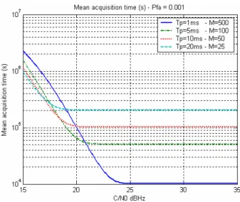
Figure 2.21: Mean signal duration required for a successful acquisition. Pfa = 1e-5, no frequency error...34
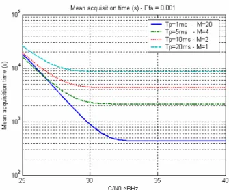
Figure 2.22: Mean acquisition time for a successful acquisition. Pfa=1e-5, no frequency error. ...35
Figure 2.23: Light indoor environment...38
Figure 2.24: 2D plot of BT-338 (standalone) in light indoor environment. ...38
Figure 2.25: 2D plot of BT-338 (MS-based) in light indoor environment ...38
Figure 2.26: Urban street environment (heading north). ...39
Figure 2.27: Urban street environment (heading south). ...39
Figure 2.28: 2D plot of BT-338 (standalone) in urban street environment. ...40
Figure 2.29: 2D plot of BT-338 (MS-based) in urban street environment. ...40
Figure 2.30: 2D plot of BT-338 (standalone) in urban dynamic test...40
Figure 2.31: 2D plot of BT-338 (MS-based) in urban dynamic test...40
Figure 2.32: AGPS tracking result of a pedestrian going outside / inside buildings. ...41
Figure 2.33: HSGPS tracking result of a pedestrian going outside / inside buildings...41
Figure 3.1: Inertial (I), ECEF (e) and navigation (n) frames. ...46
Figure 3.2: Navigation (n) frame. ...46
Figure 3.3: Euler’s angles definiton...49
Figure 3.4: Estimated inclination angle error as a function of several accelerometer biases. ...52
Figure 3.5: Accelerometer inclination measurement scheme. ...52
Figure 3.6: Euler’s angles singularity issue. ...53
Figure 3.7: Euler’s angles singularity resolution. ...53
Figure 3.8: Xsens motion tracker and sensors performance. ...54
Figure 3.9: Accelerometers turn-on bias...55
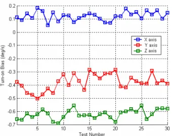
Figure 3.11: Gyroscopes turn-on bias. ...56
Figure 3.12: Gyroscope triad static outputs. ...56
Figure 3.13: Rotation rate of (e) with respect to (I) expressed in (n). vN=vE=140 km/h, h=0...58
Figure 3.14: Rotation rate of (e) with respect to (I) expressed in (n). ...58
Figure 3.15: Inertial Navigation System (INS) mechanisation...60
Figure 3.16: Predicted and actual INS horizontal RMS error...62
Figure 3.17: Biases and scale factor impact on INS horizontal accuracy...62
Figure 3.18: DGPS velocity of reference. Walk n°1...66
Figure 3.19: DGPS velocity of reference. Walk n°2...66
Figure 3.20: Best parameters computed every 2 steps. Walk n°1. ...67
Figure 3.21: Best parameters computed every 2 steps. Walk n°2. ...67
Figure 3.22: Best parameters computed over 2s. Walk n°1...68
Figure 3.23: Best parameters computed over 2s. Walk n°2...68
Figure 3.24: Regression coefficients. Non-linear model. ...70
Figure 3.25: Regression coefficients. Non-linear model (close-up). ...70
Figure 3.26: Regression coefficients. Linear model. 1st method. ...70
Figure 3.27: Regression coefficients. Linear model. 2nd method...70
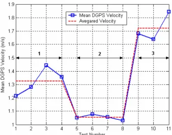
Figure 3.28: Mean DGPS velocity profile of the eleven reference tests...71
Figure 3.29: Curvilinear distance estimation error with respect to DGPS measurements...71
Figure 3.30: Mean DGPS velocity profile of the eight reference tests. ...72
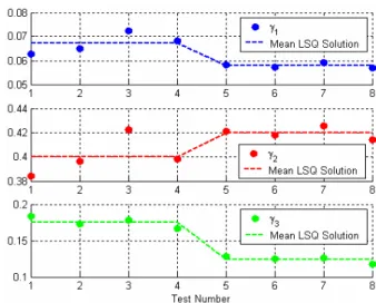
Figure 3.31: Regression coefficients. Linear velocity model. 2nd method...72
Figure 3.32: Reference velocity used for regression...73
Figure 3.33: DGPS velocity profile (up) and distance estimation error (down)...73
Figure 3.34: Regression coefficients. Linear model. 2nd method...73
Figure 3.35: Parameters of the velocity model (unit m/s). IMU is moved while walking. ...75
Figure 3.36: Relationship between the acceleration magnitude and the parameters (unit m/s2). ...75
Figure 3.37: Pedestrian Navigation System (PNS) mechanisation...76
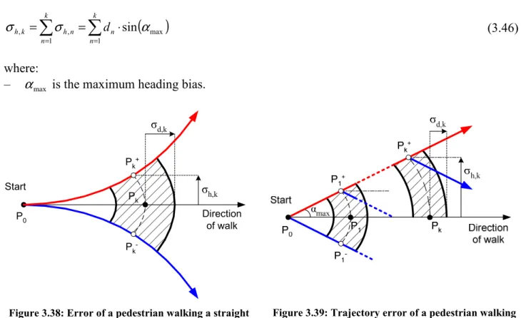
Figure 3.38: Error of a pedestrian walking a straight path assuming constant velocity and heading rate biases...77
Figure 3.39: Trajectory error of a pedestrian walking a straight path assuming constant velocity and heading biases. ...77
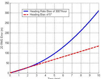
Figure 3.40: 2D upper bound position error assuming a constant velocity bias...78
Figure 3.41: Detail of the contributions of each 2D upper bound position error...78
Figure 4.1: Pressure measurement principle. ...81
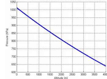
Figure 4.2: Altitude-to-pressure relationship. ...81
Figure 4.3: Required pressure resolution to enable a 1m vertical resolution...82
Figure 4.4: Impact of the pressure variation on the computed altitude...82
Figure 4.5: Altitude and temperature variations recorded over 13 hours in a closed room...83
Figure 4.6: Vertical velocity computed with the pressure sensor measurements. ...83
Figure 4.7: 3D RMS position error using pressure measurements with three different computations methods. ...84
Figure 4.8: DOPs improvement due to the processing of the pressure measurements...84
Figure 4.9: Earth’s magnetic field intensity [22]. ...85
Figure 4.10: Earth’s magnetic field declination [22]. ...85
Figure 4.11: Earth magnetic field [25]...87
Figure 4.12: Magnetic heading error with respect to inclination error. ...87
Figure 4.13: Calibration test diagram in a non perturbed magnetic environment. ...88
Figure 4.14: Magnetic field magnitude variation during the different vehicle engine start. ...89
Figure 4.16: Typical rotation rate patterns for pedestrian navigation (upper part) and land vehicle
navigation (lower part)...92
Figure 4.17: PSD of the three rotation rate components in the mobile frame (m), 1st order GM and 2nd order band-pass filter...92
Figure 4.18: Typical acceleration magnitude patterns for pedestrian navigation (upper part) and land vehicle navigation (lower part). ...93
Figure 4.19: PSD of the three acceleration components in the mobile frame (m), 1st order GM and 2nd order band-pass filter...93
Figure 4.20: Inclination filter principle...95
Figure 4.21: Heading filter principle...98
Figure 4.22: Attitude filter algorithm using all the sensors. ...100
Figure 4.23: Attitude filter algorithm with only 1 gyroscope in the sensors unit. ...101
Figure 4.24: Attitude filter heading solution...102
Figure 4.25: Normalised magnetic field magnitude...102
Figure 4.26: Attitude filter and gyro-based heading errors. All sensors are used...103
Figure 4.27: Attitude filter heading error. All sensors used...103
Figure 4.28: Trajectories using different heading sources. Pedestrian case with the triad of gyroscopes...104
Figure 4.29: Attitude filter and gyro-based heading errors. Only one gyroscope is used. ...105
Figure 4.30: Y axis gyro bias estimate of the Inclination Kalman Filter (IKF)...105
Figure 4.31: Trajectories using Different Heading Sources. Pedestrian Case with only one Gyroscope. ...106
Figure 4.32: Heading errors with respect to the DGPS reference. All the sensors are used...107
Figure 4.33: Trajectories using different heading sources. Land vehicle case with three gyroscopes. ...107
Figure 4.34: Trajectories using different heading sources. Land vehicle case with only one gyroscope. ...108
Figure 4.35: ZUPT. Theoretical velocity error profiles. ...110
Figure 4.36: ZUPT. Theoretical position error profiles. ...110
Figure 5.1: Navigation systems integration principle. ...113
Figure 5.2: Satellite position definition with respect to the user’s position...116
Figure 5.3: Satellite Doppler uncertainty. GPS time known at ±2s...117
Figure 5.4: Satellite Doppler uncertainty. User’s position uncertainty of ±15km...117
Figure 5.5: Satellite Doppler uncertainty. GPS time known at ±2s. User’s position uncertainty of ±15km. ...117
Figure 5.6: Satellite Doppler uncertainty. GPS time known at ±2s. Results with real GPS ephemeris. ...117
Figure 5.7: Local Oscillator drift (ProPak GL2plus, static test case). ...118
Figure 5.8: Frequency bins and number of frequency bins to explore with respect to a user Doppler uncertainty of +/- 250 Hz...119
Figure 5.9: Sliding window variances computed from three different acceleration magnitude sources...121
Figure 5.10: Illustration of elevation (left) and azimuth (right) errors for a user’s position uncertainty of ±15km and a GPS time of ±2s...122
Figure 5.11: Bad satellite geometry configuration with respect to the user’s heading...124
Figure 5.12: Typical issue of the user’s velocity estimation. Land vehicle case...124
Figure 5.13: Drift-free attitude filter with in motion alignment aiding. ...125
Figure 5.14: Attitude angles error with respect to the estimated angles with a static initialisation of the filter. ...126
Figure 5.15: Close-up on the first epochs. The convergence of the filter is shown here and lasts
about 10 seconds. ...126
Figure 5.16: User’s Doppler uncertainty reduction procedure. ...126
Figure 5.17: User’s Doppler prediction accuracy using filtered (a) and gyro-based (b) attitude as well as the modelled pedestrian velocity. The reference user’s Doppler is taken from GPS measurements...128
Figure 5.18: User’s Doppler prediction accuracy using filtered and gyro-based attitude and the Doppler model of equation (5.7). The reference user’s Doppler is taken from GPS measurements...128
Figure 5.19: Reduction of the number of user’s Doppler bins with respect to different coherent integration times for an initial uncertainty of ±250 Hz using data provided by MEMS senors. ...129
Figure 5.20: User’s velocity estimation using all possible combinations of measurements from two GPS satellites. ...130
Figure 5.21: User’s Doppler prediction accuracy using the filtered attitude. ...130
Figure 5.22: Improvement of the combination of MEMS. ...131
Figure 6.1: Loose coupling integration scheme. Open-loop architecture. ...136
Figure 6.2: Loose coupling integration scheme. Closed-loop architecture...136
Figure 6.3: Tight coupling integration scheme. Open-loop architecture. ...137
Figure 6.4: Tight coupling integration scheme. Closed-loop architecture...137
Figure 6.5: Hybridisation architecture using external measurements for correction purposes...138
Figure 6.6: IMU placement with respect to the vehicle...141
Figure 6.7: Simplified INS mechanisation for land vehicle navigation...142
Figure 6.8: Integrated Navigation System mechanisation as designed for land vehicle navigation. Closed-loop architecture. ...148
Figure 6.9: Reference trajectory (red) and OEM4 position solution (blue). Urban trial. ...149
Figure 6.10: Different heading estimates as computed during the urban trial...150
Figure 6.11: Standalone Inertial Navigation System position solutions using different heading sources...150
Figure 6.12: INS/GPS position solution using filtered and non-filtered heading. Two Doppler measurements used for hybridisation when available...151
Figure 6.13: Integrated Navigation System trajectory. 2 Doppler and 2 pseudorange measurements used when available. ...152
Figure 6.14: Biased (red) and unbiased (blue) along track velocity profile. ...153
Figure 6.15: Two particular velocity profile discontinuities...153
Figure 6.16: Satellite geometry issue...154
Figure 6.17: Along track velocity profile corrected by the Inertial Navigation System when bad satellites configurations are detected. ...154
Figure 6.18: Corrected and non-corrected Integrated Navigation System trajectories. 2 Doppler measurements used for hybridisation when available...155
Figure 6.19: Vertical performance of the Integrated Navigation System (upper plot). Vertical profile of the exercised trial (lower plot)...156
Figure 6.20: Static errors of three different inertial navigation algorithms using low-cost sensors.159 Figure 6.21: Position solutions as provided by three different navigation systems. Short dynamic test. ...160
Figure 6.22: PNS position solutions using 100% of GPS data for velocity model calibration. Long dynamic test. ...160
Figure 6.23: PNS horizontal RMS error. Long dynamic test...161
Figure 6.24: PNS position solutions using the first 10% of GPS data for velocity model calibration. Long dynamic test...161
Figure 6.25: Unconstrained navigation solutions. ...162
Figure 6.26: Displacement direction detection result. ...163
Figure 6.27: Possible measurement configurations. ...169
Figure 6.28: Real time sensor fusion architecture (closed-loop loose coupling architecture)...169
Figure 6.29: Data synchronisation principle. ...170
Figure 6.30: Integrated Pedestrian Navigation System...171
Figure 6.31: Real time Pedestrian Navigation System interface [53]...171
Figure 6.32: HSGPS tracking performance in urban and indoor environments. ...172
Figure 6.33: AGPS tracking performance in urban and indoor environments. ...172
Figure 6.34: HSGPS/IMU hybridisation results. ...172
Figure 6.35: AGPS/IMU hybridisation results. ...172
Figure 6.36: Pedestrian trial inside and outside buildings. AGPS single point position solution (blue) and reference trajectory (yellow outdoors, orange indoors)...173
Figure 6.37: AGPS/IMU hybridisation. Long test...174
Figure 6.38: GPS measurements availability and regression coefficients (unitless) without variability detection (real time results). ...175
Figure 6.39: GPS measurements availability and corrected regression coefficients (unitless) after variability detection (post processing results)...175
Figure 6.40: AGPS/IMU hybridisation results. Long test with corrected regression coefficients (post processing results)...176
List of Tables
Table 1.1 – Applications of MEMS Accelerometers and Gyroscopes in Consumer Products [54]....2 Table 2.1: Light indoor cold start test results...38 Table 2.2: Light indoor tracking test results. ...38 Table 2.3: Urban street cold start test results ...39 Table 2.4: Urban street tracking test results...39 Table 3.1: Accelerometer triad turn-on biases and scale factors. ...55 Table 3.2: Gyroscope triad turn-on biases. ...56 Table 3.3: Candidate parameters to the pedestrian velocity model. ...65 Table 3.4: Correlation results. Parameters computed each step. ...67 Table 3.5: Correlation results. Parameters computed every 2 steps. ...67 Table 3.6: Cross-correlation coefficients (1 step)...68 Table 3.7: Cross-correlation coefficients (2 steps). ...68 Table 3.8: Distance estimation accuracy – Method 2. ...71 Table 3.9: Pedestrian mechanisation simulation parameters. ...78 Table 4.1: Toulouse Earth’s magnetic field characteristics (year 2005) [22]...85 Table 4.2: Measurement unit configuration given typical test cases. ...102 Table 5.1: Number of frequency bins to explore given an initial user’s Doppler uncertainty of ±250Hz. Pedestrian navigation case. ...129 Table 5.2: Number of frequency bins to explore given an initial user’s Doppler uncertainty of ±250Hz. Land vehicle navigation case. ...131 Table 6.1: Typical Allan constants for different types of oscillators (units of seconds) [44]...146 Table 6.2: OEM4 tracking performance in urban environment...149
Abbreviations
AGPS ... Assisted Global PositioningSystem
AOA ... Angle of Arrival BER... Bit Error Rate
BTS ... Base Transceiver Station C/A... Coarse/Acquisition
CDF... Cumulative Density Function CGI... Cell Global Identity
COO ... Cell of Origin
DCO ... Digitally Controlled Oscillator DFT ... Discrete Fourier Transform DLL... Delay Lock Loop
DoF... Degree of Freedom DOP... Dilution of Precision DSP ... Digital Signal Processor EARS ... Euler’s Angles Singularity
Resolution
ECEF... Earth-Centred Earth-Fixed ECEF... Earth-Centred Earth-Fixed EKF ... Extended Kalman Filter E-OTD... Enhanced Observed Time
Difference
FFT... Fast Fourier Transform FLL... Frequency Lock Loop GNSS ... Global Navigation Satellite
System
GPS ... Global Positioning System GSM... Global System for Mobile
communications
HDOP... Horizontal Dilution of Precision HSGPS ... High-Sensitivity Global
Positioning System IF ... Intermediate Frequency ILSQ... Iterative Least SQuare IMU... Inertial Measurement Unit INS ... Inertial Navigation System ISA ... Inertial Sensor Assembly LBS ... Location Based Services LMU... Location Measurement Unit LO ... Local Oscillator
LoS ... Line of Sight LSQ ... Least Square
MEMS... Micro Electro Mechanical System MIM ... Magnetic Interference Mitigation MSL ... Mean Sea Level
OTD ...Observed Time Difference PDA ...Personal Digital Assistant PDF ...Probability Density Function PDR...Pedestrian Dead-Reckoning PLL ...Phase Lock Loop
PND ...Personal Navigation Device PNS ...Personal Navigation System PPM ...Parts Per Million
PPS...Precise Positioning Service PRN...Pseudo Random Noise PSD ...Power Spectral Density
RAIM ...Receiver Autonomous Integrity Monitoring
RTD ...Relative Time Difference SIS...Signal in Space
SMLC...Service Mobile Location Center SNR...Signal to Noise Ratio
SPS...Standard Positioning Service TOA ...Time of Arrival
TTFF ...Time to First Fix UMTS ...Universal Mobile
Telecommunication System VDOP...Vertical Dilution of Precision
Chapter 1: Introduction
1.1 Background
Service sets around the location of a mobile, often referred as Location Based Services (LBS), are currently gaining more and more importance in the all day life. First driven by regulation issues under the E911 law dedicated to provide a location mean to the emergency call, many commercial applications or services are available today. Some are aimed at reaching a large public with mass-market perspectives such as in-vehicle or personal navigation, the others focus on specific applications such as fleet management, e-tourism, and location of workers…
Several techniques can be used to enable the location of one user in many environments. Among them, GPS-based techniques are today very attractive due to the great effort made by the industry to miniaturise front-ends and processing cores into one single chipset while increasing both acquisition and tracking sensitivity and availability of the position solution especially in urban environments. Software-based solutions are also taking more and more importance since they offer more flexibility and cost effective means to enable GPS in handsets, even if they require today non negligible computational load. The recent convergence of wireless communication providers and cell-phone industry roadmaps also tremendously accelerate the use of the GPS-based positioning techniques and more specifically Assisted GPS (AGPS). For all these reasons, it seems obvious that satellite-based techniques will become an essential part of seamless positioning systems.
However, GPS-based positioning techniques still encounter issues in indoor areas where users are very likely to go in. The processing of GPS signals is indeed very challenging as the chipsets have to deal with signals of very weak power. Receivers have to use long coherent integration time to reduce the effect of noise and increase the probability of detecting a specific satellite signal, but it makes them very sensitive to local oscillator stability, user’s Doppler contribution as well as cross-correlation peaks that might be wrongly considered as a true correlation one (often referred as near far effect). Strong multipath may also affect incoming signals, reducing at the same time the accuracy of the position solution.
As a consequence, even if GPS is a good mean to fulfil the needs of most of location applications, it still encounters big issues in harsh environments. It is therefore very likely in many indoor cases to have a complete interruption of the positioning service. In order to get the position a user whatever his location, alternative systems shall be coupled with GPS. Many exist based on the processing of WIFI, UWB, pseudolites, TV or mobile phone signals, with all different accuracies. However, all the previously mentioned augmentations require infrastructure that can largely be found in urban environments but certainly not in rural areas making indoor location still an issue.
Self-contained augmentations have the advantage of being available wherever the user is. Inertial sensors, and more generally small sensors, are the typical example of self-contained augmentation that does not require any extra infrastructure to give information about the motion experienced by a mobile. As they are currently gaining more and more importance in many products, their use to support or replace GPS inside buildings can be a great opportunity to improve the performance of the positioning system, even if their respective intrinsic performance is somewhat too poor to allow traditional inertial navigation.
1.2 Motivations and Objectives
The efforts of the semiconductor industry to produce small, low consumption and powerful chipsets are bearing fruit for now a couple of years. Today, many portable devices such as PDA or cell phones are now equipped with small GPS chipsets that includes both the RF front-end and the base-band signal processor. This trend is all the more stressed in the sensor industry as the demand is far more important [54]. Automotive industry is currently the leading sector that drives the design and the performance of the mass market sensors, but applications at consumer level are taking more and more importance. Table 1.1 illustrates the recent needs for accelerometer and gyroscope sensors in consumer products according to [54].
Consumer
product Function Examples of products
MEMS inertial device(s)
Status of commercialisation
Cell phones
Pedometer, image rotation, menu scroll, gaming, free-fall detection (HDD protection), navigation
NTT DoCoMo pedometer (2003) Vodafone image rotation (2004) Samsung SGH E760, Nokia 3230 (navigation and gaming)
2- or 3-axis accelerometer, 1- or 2-axis gyroscope Accelerometer in cell phone since 2003 Gyroscope expected in 2007–2008
PDA Navigation IMU, Web content navigation Toshiba PocketPC e740 2- or 3-axis accelerometer 2-axis gyroscope Demonstrator in 2002 at Paris PDA show Digital Still
Cameras (DSC) Image stabilisation
All Panasonic DSCs, e.g. Lumix ($200), Pentax Optio A10 ($350) Canon, Sony DSCs
Two 1-axis gyroscopes or one 2-axis gyroscope Two 2-axis accelerometers
Gyroscope established since late 1990s Accelerometer emerging Camcorders Image stabilisation, free-fall detection (HDD protection) Upper end: Panasonic (over $1500) High end: JVC 30Gb, Toshiba 60Gb Two 1-axis gyroscopes or one 2-axis gyroscope Gyroscope established since late 1990s
Laptops Free fall detection (HDD protection), GPS
dead-reckoning assist (anti-theft) IBM, Toshiba, Apple laptops 2- or 3-axis accelerometer
Free-fall detection established Other applications emerging MP3 players Free fall (HDD protection) iPod with hard disc drive 3-axis accelerometer Established Others: toys,
games, personal transporter, robots
Realistic motion
Nintendo’s Kirby “Tilt-n-Tumble” GameBoy, Microsoft gamepad “Sidewinder Freestyle Pro”, Segway, Sony Aibo robot, Sony PS3
2- or 3-axis accelerometers,
1- or 2-axis gyroscopes Established
Table 1.1 – Applications of MEMS Accelerometers and Gyroscopes in Consumer Products [54].
The use of such sensors is all the more interesting as the sensor industry is constantly improving their integration in small packages while lowering their power consumption. Three-axis accelerometers are now widely available, as for instance [56], as well as three-axis magnetometers [57]. Gyroscopes are more difficult to integrate in a single chip due to the more complex measurement procedure. However, a major integration step has been reached with the recent announcement of mass production of a two-axis low cost gyroscope [55] in a single small die.
At the time this thesis started, the market perspectives of MEMS inertial sensors were obviously not known but somewhat expected due to the increase of their use in consumer products. Furthermore, the packaging of these low-cost sensors was already small enough to make them easily incorporable in Personal Navigation Devices (PND) such as cell phones, PDA even GPS for cars. Studying the pertinence of their use to supply GPS in order to meet LBS requirement was therefore already motivated.
evolutions has strengthened the idea that they could represent a cost effective augmentation system. The use of such small sensors in combination with hardware-based or software-based GPS receivers is very likely to become a real low-cost possibility in a quite near future. As a result of these motivations, several objectives were set along this thesis with respect to typical navigation use cases. They all can be summarised in three main categories.
Given a set of low-cost sensors, a first objective was to determine what improvement could be brought in the different inertial navigation algorithms used for land vehicle or pedestrian navigation in order to enhance the navigation systems performance. Several points were of particular interest, and more specifically those listed below:
• The effectiveness of using a pressure sensor.
• The effectiveness of using a triad of magnetometers.
• The possibility of reducing the impact of the typical errors that dramatically affect the inertial navigation systems (gyroscope biases, accelerometer biases).
• The performance of self-contained augmentations based on the set of low-cost sensors.
A second objective was to analyse the feasibility of combining information from the set of low-cost sensors to reduce the HSGPS/AGPS processing core complexity or equivalently computational load when dealing with weak signals. The following points were consequently investigated:
• Improvement of the acquisition stage (especially in cold start mode) within the scope of a software-based receiver.
• Decrease of the Time to First Fix using the external set of low-cost sensors.
• Decrease of the computational load / increase of sensitivity.
Finally, the last objective was to get insights of several hybridisation schemes. The main goal was to improve the position solution availability and accuracy in harsh environments where GPS modules (either HSGPS or AGPS) can not provide accurate and reliable position solutions. The following points were thus addressed:
• Investigation of the feasibility of integrating the set of sensors in handheld devices.
• Improvement of both availability and reliability of the position solution as provided by the integrated navigation system.
• Use of very few GPS measurements to enable the correction of the error affecting the low-cost sensors output.
• Research of criteria to monitor the quality of GPS measurements in the perspective of GPS/INS hybridisation for Pedestrian Navigation System.
1.3 Contributions
The different topics studied in this thesis are detailed throughout the report. Here are summarised the main subjects that were investigated. Some of these points have been published in conferences (papers published are mentioned in the different chapters of this report – see the bibliography for details).
• Simulation of the performance of a software-based AGPS acquisition stage. The main goal of this simulation methodology is to assess the performance that can be expected from a software-based AGPS in order to estimate the computational load for a given use case and consequently the acquisition time performance of such a receiver in typical urban / indoor environments.
• Analysis of the performance of both HSGPS and AGPS in typical urban environments. This analysis is done through field test trials in real conditions in order to analyse the performance of the Assisted solution with respect to the High Sensitivity one in terms of time to fix and accuracy. In the same time, the position solutions quality is compared to determine which module is more suited to hybridisation with the low-cost sensors.
• Optimisation of INS algorithms for both land vehicle and pedestrian navigation. An exhaustive analysis of the mechanisations is provided with a particular focus on the Pedestrian Navigation System (PNS). A detailed analysis of the relationship between parameters computed from the acceleration magnitude and the velocity of the pedestrian is done, aiming at elaborating a simple but reliable model that is used to compensate for accelerometer biases.
• Euler’s angle singularity resolution algorithm. Within the scope of this thesis and in the particular case of the pedestrian navigation, the possibility of combining a GPS chipset with low-cost sensors in a handheld device is investigated. As a consequence, the Portable Navigation Device (PND) may experience all possible attitudes including those introducing singularity in the computation of the Euler’s angles (and so the heading). A specific compensation algorithm is described in the thesis that prevent from using an unreliable heading information caused by pitch angle values of +/-90°, allowing the tracking of the heading of a PND while moved during the walk.
• Improvement of the heading accuracy. An attitude filter capable of estimating the gyroscope biases as they occur during the motion is provided in this thesis. The capability of estimating these biases while the unit is in motion is especially addressed and discussed. This filter includes the Euler’s angles singularity resolution algorithm mentioned above. It also includes a magnetic mitigation technique that prevents magnetic interferences from dramatically degrading the heading accuracy, especially when the user is nearby iron objects.
• Tracking of the pedestrian heading with respect to a moving handheld device. If the PND contains the low-cost sensors that shall be combined with GPS data to provide an integrated navigation system, and because the PND may be handheld while the user is requesting its location, the heading of the PND may differ from that of the user. An algorithm dedicated to keep track of the true pedestrian heading is proposed for medium handset motions.
• Analysis of the improvement brought by the use of a barometer. The possibility of using a pressure sensor in order to get absolute or differential altitude measurements is studied to enhance the position solution using less than four GPS measurements. Discussion of the methodology used to incorporate the altitude measurements is also done.
• Improvement of the GPS acquisition stage. The processing of attitude and velocity information provided by the sensors assembly is used to estimate the user’s Doppler, which consequently allow a reduction of the number of Doppler bins to explore and therefore reduces the acquisition complexity. The capability of the attitude filter to provide sable attitude measurements is tested within this contribution for “on-demand” user’s Doppler estimation.
• Tight integration architecture taking advantage of very few GPS measurements. Designed for land vehicle application, the proposed tight integration architecture is demonstrated to allow the navigation using only 2 Doppler measurements, but accumulating errors. As soon as 2 pseudoranges are added, the integrated navigation system does not accumulate errors anymore and accuracy within 40m from the reference trajectory is shown possible with low-cost sensors. However, the proposed hybridisation architecture is very sensitive to geometry of the satellite used in the integration filter.
• Real time low-cost sensors/AGPS (or HSGPS) integrated pedestrian navigation system. A real time integrated navigation system prototype that fuses MEMS sensors with AGPS (or HSGPS) is developed to ease the characterisation of such a seamless positioning system especially in outdoor to indoor and indoor to outdoor transition phases. Several GPS quality monitoring criteria are proposed and their pertinence is tested on actual data, which demonstrated a 2D error within 10 metres from the reference trajectory even during GPS outage of about 2 minutes.
1.4 Thesis Outline
This thesis report is organised as follows:
Chapter 2 recalls the basics of the GPS positioning techniques and gives insights of current enhancements in the processing core of mass-market receivers such as HSGPS and AGPS. Simulations are done to estimate signal processing performance such as time to fix with respect to typical satellite configurations. Both types of low-cost receivers are tested in urban and indoor environment to assess their respective performances and find the module that gives the best ones.
Chapter 3 introduces the alternative navigation systems based on inertia principles. First the classical Inertial Navigation System (INS) mechanisation is derived in details and its performance relative to the quality of the sensors used within the scope of this thesis is discussed. The particular case of the pedestrian navigation is then addressed in great details and the mechanisation chosen in the thesis is justified. The performance of such a mechanisation is simulated according to several error models and compared to what can be obtained using the classical INS.
Chapter 4 deals with the possible self-contained augmentations that can be implemented in order to improve the performance of the algorithms described in chapter 3. In particular, the addition of a pressure sensor and magnetometers are discussed. Several well-known error limitation principles are recalled. This chapter focuses also on the dynamic estimation of gyroscope drifts and an attitude filter capable of providing stable heading information is proposed. The possibility of mitigating magnetic interferences is also addressed.
Chapter 5 focuses on the improvement of the HSGPS/AGPS processing stage and more specifically on the acquisition stage. The different Doppler contributions affecting the incoming signal are analysed, with more attention paid to that of the user. The possibility of estimating the user’s Doppler prior to engage the acquisition process and assuming the unit containing both the GPS chipset and the sensors assembly in motion is then investigated. The sensors fusion algorithm is tested for pedestrian and land vehicle navigations. Both static and dynamic cases are studied.
hybridisation of the different navigation systems described in chapter 2 and chapter 3. The land vehicle navigation case is studied through a tight integration scheme which differs from the standard one usually used to fuse GPS and INS. The pedestrian navigation case is addressed through a loose coupling scheme. A real time pedestrian navigation system is developed for that purpose. These different hybridisation algorithms are tested in typical urban conditions and respective performance results are detailed.
Chapter 2: GPS-Based Positioning
This chapter is dedicated to the presentation of the GPS-based positioning technique for personal positioning. In a first part, the GPS fundamentals are recalled and a focus is put on the measurements available at the output of a GPS receiver for further integration with another navigation system and more specifically with an Inertial Navigation System (INS). The main processing stages of a standard GPS receiver are then briefly presented. In a third time, new architectures such as HSGPS and AGPS are discussed. The weakest points of the standard GPS processing are highlighted and solutions implemented in the new processing architectures are described. The performance of each type of positioning method is finally discussed in terms of time to acquire, time to fix and position accuracy. A comparative test between HSGPS and AGPS is also presented in typical indoor environments and the need for augmentations in harsh environment is demonstrated.
2.1 The Global Positioning System
2.1.1 Fundamentals
The Global Positioning System (GPS) is a satellite radionavigation system that can provide any user on Earth at any time with the signals necessary for an accurate determination of its position, velocity as well as the bias of its own clock, independently of weather conditions.
The basic principle of getting its position using GPS relies on range measurement. A user equipped with a receiver computes its location by measuring the delay of propagation of the signals coming from several transmitting satellites. These satellites have a known position, so that once the clock bias of the local receiver oscillator with respect to the satellite transmitter has been solved, these propagation delays can be converted into geometric distance, allowing the resolution of the 2D / 3D user’s position. The velocity of the user can also be computed using the rate of change of these propagation delays.
In such a positioning system, timing is a very critical point. Indeed, the satellites are transmitting permanently continuous waveforms (the GPS signal) that are designed to be easily related with a time scale. Transmitters and receivers are aware of the signal characteristics and properties, so that the demodulation of the GPS navigation message is done trough a processing designed to take advantage of the GPS signal modulation. The propagation delay is thus measured by comparing the received signal to a locally generated copy of that signal. However, as the receiver clock is not synchronised with the satellites clocks, the time delay measurement is biased by the clock bias between the receiver and the satellite. Thus, in order to determined that bias, GPS satellites broadcast in their navigation message satellite clocks biases with respect to that reference time. As a consequence, the propagation measurements can be considered to be only biased by the receiver clock bias so that this remaining unknown is just simply added to the three basic unknown user’s coordinates. Four satellites are thus at least needed to compute the user’s location.
GPS is composed of three segments defined as space, control and user. They all are described in the following subsections.
2.1.1.1 Space Segment
The space segment is the satellite part of the positioning system. It is composed of 24 satellites orbiting in 6 different orbit planes inclined at about 55°, with a radius of about 26600km [1]. The period of revolution of a GPS satellite is 12 sidereal hours, so that the ground track of each satellites is repeated every 24 sidereal hours, that is 23h56min. The satellite payload contains four atomic clocks, two based on Rubidium and two on Caesium, for a precise signal generation. The satellites are currently emitting a signal propagated on two carriers (L1, L2) with the following properties:
– L1 at 1575.42MHz with a QPSK modulation. The in-phase channel is modulated by a known Gold code of length 1023, the C/A code, with a rate of 1.023MHz. The quadrature channel is modulated by a known P code or unknown encrypted version Y code, both clocked at 10.23MHz.
C/A codes are widely known so that the service provided through the L1 C/A carrier called Standard Positioning Service (SPS) is accessible by everybody. Opposite, the Precise Positioning Service (PPS) supported by L2 and the quadrature channel at L1 is reserved to US military and their allies since they are the only ones capable of decoding the Y code. The service provided on L2 and L1 with the P(Y) code is not within the scope of this thesis. Consequently, the following will focus on the L1 C/A carrier.
All the satellites use the same frequencies to transmit the GPS navigation message. The generation of the L1 signal is as described below in Figure 2.1. The transmitted signal is the result of the 2-modulo sum of the spreading codes c and p (or y) and the navigation message d, which are then QPSK modulated. The spreading code c used on GPS modulation is a Gold code, with length N=1023 bits. Its rhythm is larger than the data rate, so that the modulation is a spread spectrum modulation.
Figure 2.1: GPS L1 signal generation architecture.
The signal transmitted on L1 by the GPS satellite i is a combination of the C/A and P(Y) codes, which is 3dBW lower than the C/A component. Omitting the P(Y) component, the GPS L1 signal transmitted by satellite i is then as written in equation (2.1):
(
Lt)
t c t d A t si( )= ⋅ i( ) i( )cos 2π 1 (2.1) where: − id is the P/NRZ/L materialisation of the satellite i navigation message at 50 Hz.
− i
c is the P/NRZ/L materialisation of satellite i C/A code at 1,023 MHz.
− m is the P/NRZ/L materialisation waveform.
− A is the amplitude of the C/A component.
It is then straightforward to compute the Power Spectral Density (PSD) of the signal transmitted on L1, according to equation 2.1. The L1 PSD is thus as follows [3]:
( )
( )
( )
− + + ⊗ ⊗ ⋅ = 4 ) ( ) ( 1 1 2 f L f L f S f S A f S d c si δ δ (2.2) where:– Sd( f) is the PSD of the GPS navigation data. – Sc( f) is the PSD of the C/A code.
– f is the repetition frequency of the spreading code c. R
The PSD of the base band C/A component Sdc(f)=Sd
( )
f ⊗Sc( )
f is plotted in Figure 2.2. The total bandwidth of the transmitted GPS signal on L1 is larger than 20 MHz. Due to the spreading code properties, the spectrum lies below the noise spectrum.Figure 2.2: Baseband C/A PSD.
2.1.1.2 Control Segment
The role of the control segment is to ensure the surveillance of the received signal characteristics, to compute the ephemeris data and the satellites clock corrections, and to download the navigation message into the satellites payload. The control segment is composed of 5 surveillance stations scattered around the globe, 1 main control station called the Master Control Station (MCS) located in Colorado, 4 download stations. These stations perform normally 1 download per day per satellite, with the possibility to do 3 downloads per day per satellite.
Subframe 1 TLM HOW GPS Week Number - Space Vehicle Accuracy and Health - Satellite Clock Correction Terms
Subframe 2 TLM HOW Ephemeris Parameters
Subframe 3 TLM HOW Ephemeris Parameters
Subframe 4 TLM HOW Almanac and Health Data for Satellites 25-32, Special Messages, Satellite Configuration Flags, and Ionospheric and UTC Data
Subframe 5 TLM HOW Almanac and Health Data for Satellites 1-24 and Almanac Reference / Time and Week Number
30 bits
300 bits
Figure 2.3: Structure of a GPS frame.
The navigation message generated for each satellite is necessary for the receivers to compute Noise level
the position and the velocity of the user. This 50 bits per second data stream is synchronous with the 1 kHz C/A spreading code epochs. The navigation message is periodic. It contains 37500 bits, and thus, lasts 12,5 min. The data is formatted into 30-bits word, and words are grouped into subframes of 10 words. A subframe is then composed of 300 bits, and lasts 6 seconds. Five subframes form a frame. Therefore, a frame is composed of 1500 bits, and lasts 30 seconds. Frames are grouped together, and the 25 frames of 37500 bits compose the navigation message. Figure 2.3 illustrates the navigation message structure.
In the message, much of the data is repeated every frame, and some every subframe. The navigation dataframes are periodically updated, approximately every 2 hours, and are valid for 4 hours. According to the above description, it is clear that without any external aid, the minimum time required for a receiver to incorporate the pseudorange measurements made on a new specific satellite in the position solution is then 30 seconds because satellite clock correction and ephemeris data are repeated in each frame. Details about the messages can be found in [1].
2.1.1.3 User Segment
That segment is composed of the authorised users (military) and non-authorised users (civilians). The receivers can be static on Earth, or mobile in a vehicle on Earth, in an aircraft or a spacecraft. They permanently collect GPS signals and process them to compute the position and velocity of the user. At the input of the receiver’s antenna and compared to what is transmitted by the different satellites, the GPS signals are affected by delays accumulated during the different phases of the propagation. At the output of the receiver’s antenna, the signal is as follows:
) ( ) ( ) ( ) ( ) (t g t s t w t j t r = ⊗ + + (2.3) where:
− g is the pulse response of the propagation channel.
− w is an additive white noise.
− j is the sum of the jammer signals.
Assuming that the propagation channel modifies the received signal such as g is a pure delay (g(t)=δ(t−τ)), at the output of the receiver’s antenna, the complete expression of the continuous
signal is then given by equation (2.4):
(
2)
( ) ( ) cos ) ( ) ( ) ( 1 1 1 0 t w t j t L t c t d A t r i ki ki N i M k i k i i k i + + − ⋅ − ⋅ − ⋅ =∑ ∑
= − = θ π τ τ (2.4) where: − i kA is the amplitude of the received signal at epoch k. It is time dependent.
− i k
τ is the propagation delay affecting the received signal at epoch k. It is time dependent.
− i k
θ is the carrier phase shift, including Doppler effect at first order at epoch k.
− N is the number of received satellite signals.