OATAO is an open access repository that collects the work of Toulouse
researchers and makes it freely available over the web where possible
Any correspondence concerning this service should be sent
to the repository administrator: [email protected]
This is an author’s version published in:
http://oatao.univ-toulouse.fr/24136
To cite this version:
Laouafa, Farid and Guo, Jianwei and Quintard, Michel
Underground rock
dissolution and geomechanical issues. (2019) In: 53rd US Rock Mechanics /
Geomechanics Symposium ARMA 19, 23 June 2019 - 26 June 2019 (New York
City, United States).
1. INTRODUCTION
Many problems in geomechanics such as subsidence, sinkholes and collapses, are related to the dissolution of soluble rocks. For example rock dissolution may create underground voids of large sizes, leading to a potential risk of instability or collapse, as illustrated in Fig. 1. Since dissolution of porous rocks may cause catastrophic damages, it is a major concern in geomechanics field.
Fig. 1. Land Subsidence (sinkhole) in Central Kansas related to Salt dissolution (after USGS water science).
In many cases, dissolution is driven by an under saturated fluid flow. For instance, the subsurface water flow or hydraulic conditions through soils and rocks determines the onset conditions of geomechanical instability. Moreover, the natural or man-made hydraulic condition may evolve with time and change in space. Dissolution is also used intensively, for example in case of solution mining of salt. This industrial process extracts underground salt, by injection of fresh water through an injection well and extraction of the saturated brine at an extraction well. This process is very suitable in case of thin salt layer located at great depth.
The multi-scale and multiphysics features of rock dissolution problem raise many questions. The first of them concerns the accuracy needed in the description of solid-liquid interface recession at the macro-scale level (Darcy-scale). To achieve this goal, a precise mathematical formalization of physicochemical and transport mechanisms at the micro-scale level is required. The second one is linked to the description of dissolution at large spatial scale (in situ scale, site scale). The third one deals with strong physical couplings with other processes, in particular, mechanical behaviors of rocks.
Underground rock dissolution and geomechanical issues
Laouafa, F.
Institut National de l'Environnement Industriel et des Risques- INERIS (France) ; Verneuil-en-Halatte, F-60550, France
Guo, J.
School of Mechanics and Engineering, Southwest Jiaotong University, 610031 Chengdu, China
Quintard, M.
Université de Toulouse ; INPT, UPS ; IMFT (Institut de Mécanique des Fluides de Toulouse) ; Allée Camille Soula, F-31400 Toulouse, France and CNRS ; IMFT ; F-31400 Toulouse, France
ABSTRACT:
This paper deals with the problem of the dissolution of soluble underground rocks and the geomechanical consequences such as subsidence, sinkholes and underground collapse. In this paper, the rock dissolution and the induced underground cavities are modeled using a Diffuse Interface Model. We describe briefly the method. We used to perform the transition (upscaling) from a multiphysics problem formulated at the microscopic scale level (pore-scale) to the macroscopic scale level (Darcy-scale). Rock material considered in this paper is gypsum, despite that the developed method is also suitable for more soluble rocks. The mechanical consequences of dissolution are analyzed for two theoretical configurations, i.e., lens and pillar.
The main dissolution rate models are often phenomenological. They are built at the macroscopic scale level. Based on laboratory tests or in-situ observations, the phenomenological dissolution models are intensively used currently. These approaches may be considered as describing in fact dissolution in an average sense. Unfortunately, these phenomenological models are unable to take into account accurately the effects of natural convection (at pore scale level) and the presence of heterogeneity at the microscopic scale, for example. This paper, presents these different questions, based on theoretical and numerical analyses of several examples. The starting point of our dissolution problem is the pore- scale description of the dissolving surface and the choice of the surface dissolution kinetics, which has been the subject of many studies for various dissolving materials, mainly in chemical or geochemical scientific domains. Generally, the reaction rate, R, applied in the boundary condition (of a boundary value problem) for the micro-scale dissolution problem for soluble rocks like limestone, calcite, gypsum, or salt follows a general form expressed as (Jeschke et al., 2001; Jeschke and Dreybrodt, 2002): 1 n eq C R k C = −
In this expression, kis the reaction rate coefficient, Cis the concentration of the dissolved species and Ceq the thermodynamic equilibrium concentration (also named solubility). This paper focuses mainly on the dissolution of gypsum (CaSO4·2H2O), even if we will sometimes refer to the dissolution of salt.
Recall that the Damköhler number (Da) is a dimensionless number, which is used in chemical engineering to relate the chemical reaction time scale (reaction rate) to the transport phenomena rate occurring in a system. When Da is very large, for instance through a very large value of k, this boundary condition tends to the classical equilibrium condition expressed by
eq
C=C at the solid surface. Assume such an approximation is valid restricted in our analyses to two different approaches for modeling the dissolution problem. The first one is an explicit following of the fluid-solid interface. This can be done using an Arbitrary Lagrangian-Eulerian (ALE) method (Donea et al. 1982). The second approach tackles dissolution using a Diffuse Interface Model (DIM) in order to smoothen the solid-liquid interface with continuous quantities (Anderson et al., 1998, Collins et al., 1985, Luo et al., 2012).
In section 2, the physical and mathematical base of the dissolution model is presented. Then the DIM model is deduced thanks to a volume averaging theory. More
precisely, the mathematical problem is formulated at the pore-scale and then upscaled to Darcy-scale in order to obtain macroscopic balance laws and the associated effective parameters. The workflow is depicted in Fig.2.
Fig. 2. Problem: From micro-scale to large-scale levels We will then discuss the analysis of the dissolution of two relatively simple cases. The first one concerns the dissolution of a cylindrical gypsum lens located under an elastoplastic overburden. We will analyze the evolution of the plasticity in the overburden as a function of the dissolution of the lens. In this same class of problem, we will analyze the subsidence when the lens is close to the surface. The second case concerns the dissolution of an elastoplastic pillar of cylindrical gypsum. We analyze the stability of this pillar according to the intensity of the dissolution. We introduce another example, for illustration, the effect of dissolution when the permeability is a function of the volumetric strain. These examples show the potentialities of the approach in the conditions of numerical weak or strong coupling between the two physics: dissolution and mechanical.
2. DISSOLUTION MODELS
This section describes first a generic pore-scale dissolution model corresponding to dissolution of a soluble solid species considered as a single component. The approach can be extended easily to a material having several components (multi-components). In this latter case, the conservation equations (mass, momentum, etc.) apply to each component of the physical system. The idea or spirit of the method will be given about the upscaling of the pore-scale equations to derive a macro-scale diffuse interface model will be given. This larger scale or Darcy-scale model can then be used to model the dissolution of large cavities or porous formations. The methodology is available for salt, gypsum and even carbonate rocks, provided local conditions are compatible with the assumption of a pseudo-component. Otherwise, the same methodology must be extended to a multicomponents treatment, which is beyond the scope of this paper.
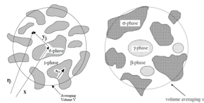
Consider two classes of dissolution models. The first one is original dissolution problem corresponding to a sharp
liquid/solid interface (Fig. 3). In this case the solid-liquid interface is defined mathematically by a surface at which the liquid concentration is equal to the thermodynamic equilibrium concentration. Introduce a scalar phase indicator defined in the whole domain (rocks and fluid), for example the porosity
ε
β, it has a value of 1 in the liquid phase and zero elsewhere, with a jump at the solid-liquid interface (Fig. 3 (left)).Solving the mathematical problem with sharp interface requires special front tracking, front marching numerical techniques, which are often computationally time consuming and are confronted with numerical difficulties, in particular in the presence of geometrical singularities (near non-soluble layers). These difficulties can be circumvented if we do not require an explicit treatment of the moving interface. Instead, partial differential equations are written for continuous variables, such as
ε
β and the mass fraction of species A in the β-phase(ω
Aβ), which lead to a diffuse interface as illustrated in Fig. 3 (right).Fig. 3. Original dissolution model (sharp interface on the left) and Diffuse Interface Model (on the right).
The original solid/liquid dissolution problem can be described by classical convective-diffusive mass balance and Navier-Stokes (momentum) equations, etc. To express the DIM model, we start from these original solid/liquid equations to generate averaged or Darcy-scale equations involving effective coefficients (Luo, et al. 2012, Guo et al. 2015) and take into account the density variation as a function of concentration. In the first subsection, the original model for the dissolution problem is introduced. In the second subsection, we briefly introduce the upscaling method leading to the “Darcy-scale” equations which are used as the basis for the DIM formulation.
2.1. The original multiphase model
Let us consider a binary liquid phase β containing chemical species A and B, and a solid phase σ containing only chemical species A.
Fig. 4: Large-scale (left) and near interface scale(right). In Figure 4 (right), v∞,v , wβ βσ,nβσ represent the velocity of the fluid far away from the interface, the velocity of the phase
β
near the interface, the recession rate, and the normal to the interface, respectively. In the following, bold letters indicate either vector or tensor variables.(
)
(
)
(
)
(
)
( ) 0 ( ) 0 ( ) 0 A A A a t b t c t β β β β β β β β σ σ σρ
ρ
ρ ω
ρ ω
ρ
ρ
∂ + ∇⋅ = ∂ ∂ + ∇⋅ = ∂ ∂ + ∇ ⋅ ∂ = v v v (1)Equation 1(a) refers to total mass balance equation for the β-phase. Equation 1(b)is the mass balance for species A in the β-phase. The general mass balance equation for a moving σ-phase is given by equation 1(c).
In terms of the fluid, we will use the Navier-Stokes equations for the momentum balance, i.e.,
2 p t β β β β β β β β
ρ
∂ + ⋅∇ =ρ
− ∇ +ζ
∇ ∂ g v v v v (2)where, vβrepresents the velocity of the β-phase, ∇pβ
the pressure gradient in the β-phase,
ζ
β the dynamic viscosity of the β-phase and g the gravity vector. At the β-σ interface Aβσ , the chemical potentials for each species should be equal for the different phases. In this case and for the special binary case under investigation, we have the following equality at a given pressure p and temperature T:(
, ,)
(
, ,)
atAβ Aβ p T Aσ Aσ p T Aβσ
µ ω
=µ ω
(3)where,
ω
Aσ is equal to 1. It must be emphasized that in the complete binary case, i.e., whenω
Aσ is not equal to1, there is also a relation similar to the above equation for the other components.
This results in the classical equilibrium condition, i.e.,
at
Aβ eq Aβσ
ω
=ω
where,
ω
eqis the equilibrium concentration for species A.From the mass balances for species A and B at the
β σ
− interface and using a theory of diffusion (Taylor and Krishna, 1993), the mass balance for species A can then be expressed as follows:(
A)
(
)
(
)
A DA A t β β β β β β β β ρ ω ρ ω ρ ω ∂ + ∇ ⋅ = ∇ ⋅ ∇ ∂ v (4)The boundary conditions for the pseudo-component mass balance at the solid-liquid interface (of outward normal nβσ can be written as a kinetic condition:
(
)
(
)
(
)
n 1 n at A A A n s eq D M k A βσ β β β βσ β β βσ βσ βσ β σω
ρ
ρ
ω
ρ ω
ω
⋅ − − ∇ = − − = ⋅ − w v w (5)wherewβσis the interface velocity and M is the molar weight of the pseudo-component, ksis the reaction rate
coefficient, n is the nonlinear reaction order. This equation can be used to calculate the interface velocity. We can remark that in general we have the following inequality: wβσ vβ
For gypsum, for instance, the maximum value of
nβσ⋅wβσ is about9.7 10 m / s,× −8 which is negligible compared to seepage velocities in hydrogeology, on the order of 10 to 10 m / s.−5 −6 A boundary condition corresponding to no jump in the tangential velocity has to be enforced at Aβσ . Therefore, considering as negligible the advected normal flux at the solid-liquid interface, the former equation is simplified into
(
)
n 1 A at n s A eq D M k β A βσ β β βσω
ρ
ω
ω
⋅ − ∇ ≈ − − (6)The recession velocity wβσ can also be expressed as follows: 1 n n (1 A ) A D βσ βσ β βσ β σ β
ω
ρ
ω
ρ
⋅ = ⋅∇ − w (7)Darcy-scale equations are obtained by upscaling the set of pore-scale equations. The reader will find in paper (Guo et al., 2016) the details of this change of scale. The last equation above relates explicitly the recession velocity to the transport flux and can be used to compute
the interface movement in ALE. The dissolution problem is completed with the set of equations to describe the boundary and initial conditions of the fluid domain. Because of the complex movement of the interface, frequent re-gridding is required and the resolution near the interface cannot be very fine or else creates rapid unacceptable distortion of the mesh. Some of the numerical difficulties associated with very sharp fronts can be circumvented by using a Diffuse Interface Method. Contrary to "sharp methods", a diffuse interface method considers the interface as a smooth transition layer where the quantities vary continuously. The whole domain constituted by the two phases is considered to be a continuous medium without any singularities nor a strict distinction of solid or liquid (see Fig.3).
2.2 Darcy-scale non-equilibrium model
In the following analysis, the σ-phase is supposed immobile, i.e.,vσ =0.
Fig. 5. Averaging volume at pore-scale level and material point position vector (left) and three-phase model (the third phase may be insoluble species for instance) (right).
The volume averaging theory (Quintard and Whitaker, 1994, Whittaker, 1999) will be used to upscale the balance equations formulated at the pore-scale (Fig. 5). We define the intrinsic average of the mass fraction as
( )
1 1 A A A A V dV V β β β β β β β βω
ε ω
−ω
Ω = = =
rand the superficial average of the velocity as
( )
1 V dV V β β β = β =ε
β β =
β V v v v rwhere Vβ is the filtration velocity and Uβ = vβ β is the β-phase intrinsic average velocity. After transformation, the averaged form of balance equation of species A can be expressed as:
(
)
( ) ( ) ( ) ( ) 1 -A A A A A A A D t dA V βσ β β β β β β β β βσ β β β ρ ω ρ ω ρ ω ρ ω ∂ + ∇ ⋅ = ∇ ⋅ ∇ ∂ ⋅ −
1442443 144424443 14243 1444442444443 c b a d v n v w (8)The different terms of (a), (b), (c) and (d) express: (a) accumulation, (b)convection, (c) diffusion, and (d)the phase exchange terms, respectively. After several assumptions and some mathematical treatments of the different equations, we have the following governing equations for the diffuse interface model (DIM) (Luo et al. 2012):
(
)
(
)(
)
* * * * * . 1 A A A A A eq A t β β β β β β β β β β β β β ε ρ ρ ε ρ ρ α ω ∂Ω + ⋅∇Ω = ∇ ⋅ ∇Ω + ∂ − Ω − Ω V D (9) and(
)
(
)
* * * eq A t β β β β β βε ρ
ρ
ρ α ω
∂ + ∇ ⋅ = − Ω ∂ V (10) and(
)
* eq A t t β σ σ σ β βε
ε
ρ
∂ρ
∂ρ α ω
− = = − Ω ∂ ∂ (11)where
ρ
β* is such thatρ ω
β Aβ =ε ρ
β β*ΩAβ andα
is the exchange term between the two phases.D*Aβ is themacroscopic diffusion/dispersion coefficient :
(
)
* I T I A L T D β β β β β β β βα
α α
τ
ε
ε
= + V + − V V D Vwhere the tortuosity,
τ
β , the longitudinalα
L ,andtransversal,
α
T, dispersivities depend on the pore-scalegeometry. The macroscopic effective coefficients are obtained by solving the “closure problems” provided by the theory over different types of unit cells representative of the porous medium, as illustrated in Fig. 6.
Fig. 6. Examples of 1D, 2D and 3D unit cells (after Courtelieris and Delgado, 2012 )
Closure problems correspond to an approximate solution of the coupled problem: averaged variables/deviations.
The approximate solution often takes the form of a mapping such as
(
)
Aβ β Aβ sβ eq Aβ
ω
% = ⋅∇Ω +bω
− Ωwhere
ω
%Aβ is the concentration deviation,bβ and sβ are the two closure variables. Solving two boundary value closure problems for bβ and sβ allows us to express the macroscopic effective values according to the characteristics at the pore-scale. In other words, the physical properties at the macroscopic level are not "phenomenological" values but built on the basis of physical properties observed ordefined at the microscopic scale.In our case, we obtain the effective macroscopic diffusion tensor D*Aβ , the macroscopic effective exchange coefficientα
and the effective densityρ
β* such as:(
)
11 1 A A A D dA b V βσ β β εβ− βσ β εβ− β β = + −
% * D I n b v(
) (
)
1 1 eq A A D s dA V βσ β β βσ βρ
α
ω
= ⋅∇ −
n * 1 A A β β β β βρ
ρ ω
ε
= ΩWe observed that when the saturation at a material point is reached, then: 0 eq A Cte t β β β
ε
ω
= Ω ∂ = ⇔ε
= ∂In the case of DIM use, i.e., not a real porous medium problem application, the choice of the exchange coefficient
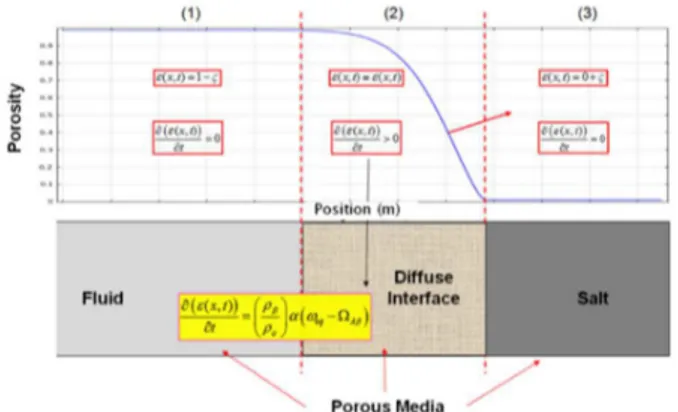
α
expression as a function of porosity is more arbitrary. It must, however, be observed a null condition when the material point is considered strictly in the fluid phase or strictly in the solid phase. This is illustrated in Fig. 7.Fig. 7. Porous domains: "fluid"-interface-solid and expression of volume fraction
ε
We must underline that, in the DIM model, there is no “pure liquid phase” (Fig. 7) since
ε
β is used continuously to represent the fluid as well as the solid regions. Therefore, the Navier-Stokes equations are no suitable in this situation. Thus, we can adopt a Darcy-Brinkman model (Darcy-Brinkman, 1947) to replace Navier-Stokes equations for the momentum balance equations( )
(
*)
( )
1 0 A A P β β β β β β β β β µ ρ µ ε − Ω ∆V − ∇ − g − Ω K ⋅V = (12)where the permeability tensor K is a function of
ε
β. The Darcy-Brinkman equation will approach Stokes equation when K is very large and will simplifies to Darcy’s law when K is very small. If inertia terms are not negligible, a similar Darcy penalization of Navier-Stokes equations may be used. The resulting DIM equations may be solved with various numerical techniques, but in this paper we will use a COMSOL® implementation. Results are presented and discussed in the next section.3. DISSOLUTION MODELING WITH GEOMECHANICAL ISSUES
The goal of this section is to show the potential application of the method. Two "theoretical" configurations are considered that are sufficiently representative of real cases.
The first case corresponds to the dissolution of a gypsum pillar in the presence of continuously flowing water. This configuration can be encountered in the case of a room with pillars in a flooded gypsum quarry with a continuous forced convection of fresh water. The second case corresponds to flow induced by a natural hydraulic gradient in a porous rock formation that contains a gypsum lens. This lens is, for instance, located in a porous medium between two layers of marl.
This study is of direct relevance to gypsum mining and natural dissolution of geological formations containing gypsum. Gypsum dissolves easily in flowing water, with time-scales on the order of years (therefore similar to human activity time-scales), so that any gypsum mine which becomes flooded on abandonment should be subject to a hydrological and geomechanical study. If a gypsum mine is fully or partially flooded, a continuous saturated or unsaturated flow of fresh water around pillars could decrease significantly their cross sections through dissolution (near the floor level in case of partial flooding) and leads to the pillar failure.
Whatever the hydrogeological configuration, dissolution of gypsum raises the question of consequences in terms of geomechanical behavior: surface subsidence, sinkholes, caverns or pillar stability, etc. The purpose of this section is to present some examples, indeed simplified, to illustrate the numerical robustness and the potentialities of the numerical dissolution approach outlined in the previous sections.
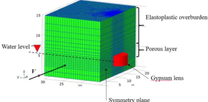
3.1. Gypsum lens - elastoplastic recovery
The problem considered is an isothermal dissolution of the cylindrical gypsum lens of height 2.5 m and diameter of 5 m (Fig. 8). The lens is located between two supposed non permeable domains (up and down), in a porous medium. The imposed upstream flow (inlet) velocity V is equal to 10-6 m/s. The concentration of the inlet fluid is zero. All the boundaries of the layer containing the lens are zero flux, with the exception of the inlet and the outlet boundaries. The permeability K of the gypsum rock is 10-15 m2 and that of the surrounding medium of 10-12 m2. The fluid dynamical viscosity is that of water (10-3 Pa.s). From a mechanical point of view, the elastoplastic (Mohr-Coulomb) overburden has a Young's modulus of 25 106 Pa, a Poisson coefficient of 0.3, a cohesion of 105 Pa and a friction angle of 30 °. The Young Modulus of the supposed elastic gypsum lens is equal to 35 GPa.
Fig. 8. Mesh and location of soluble gypsum lens.
The density of all materials is taken equal to 2000 kg/m3. The model has a vertical plane of symmetry passing through the middle of the lens (Fig. 8). As a consequence we will model only half of the domain. On all sides of the model the normal component of
displacement is zero (roller plane). The only load is gravity.
Fig. 9. Gypsum lens at different times (0, 10, 40 and 50 years). In Fig. 9 we have presented the 3D shape of the gypsum lens at different times (0, 10, 40 and 60 years). We observe a significant reduction in the cross-section induced by dissolution. For this particular hydrodynamic conditions (Darcy flow, no density effect, etc.) the initial cylindrical shape is preserved. Fig. 10 depict the evolution over time of a cross section passing through the middle of the cylindrical lens. One can also observe the circular shape that is preserved and the significant decrease of the section with time.
Fig. 10. Time (0, 20, 30, 40, 50, 60, 65 yrs) evolution of a cross section passing through the middle of the cylindrical lens.
Fig. 11. Example of spatial distribution of normalized concentration after 20 and 50 years.
The cover being elastoplastic, creating a cavity induced by dissolution may in turn induce plasticity therein. If the cavity has a significant size and/or weak mechanical properties, the effects of dissolution can result in subsidence and ultimately creating a sinkhole. In Fig. 12 and Fig. 13 we show the spatial distribution of the effective plastic strain for 3 times. Recall the expression of effective plastic strain
ε
ep :(
)
2 3 ep p p ij ij d dε
=
ε
ε
In Fig. 12 and Fig. 13, we observe the spatial extension of plastic strain in the overburden, function of lens dissolution.
Fig. 12. Effective plastic strain distribution in the recovery after 20, 40, and 60 years.
Fig. 13. Isovalues of the effective plastic strain distribution in the recovery after 20, 40, and 60 years.
Finally, we obtain (Fig. 14) the following plasticity in the recovery.
Fig. 14. Effective plastic strain distribution in the recovery after total dissolution of gypsum lens.
In Fig. 15 we show the time evolution of the volume integration of the effective plastic strain:
_ ep
Overburden
Int EP=
ε
dvFig. 15. Time evolution of the volume integration of the effective plastic strain over the overburden.
The purpose of this integration is not so much to determine a particular value from a physical point of view but to show the temporal evolution of plasticity in the recovery. This increases continuously with time (i.e. with dissolution) and remains constant when the gypsum lens is completely dissolved.
Fig. 16. 3D distribution of vertical displacement when the gypsum lens is totally dissolved.
Fig. 17 show the evolution of vertical displacement w, for point A located in the middle of the model and on the bottom of recovery and point B located in the middle of the model and on the surface.
Fig. 17. Vertical displacement w(t) function of time at two points A and B.
We observe that the vertical displacement increases as the dissolution progress. In the next subsection we consider a weak recovery and a lens located close to the surface.
3.2. Gypsum lens - subsidence
In this sub-section, we discuss the evolution of subsidence as a function of dissolution. We adopt the same boundary and initial conditions as before. The lens has now a diameter of 7.5 m and is very close to the surface (thickness of 5 m). The overburden is assumed elastic with a Young's modulus of 5 MPa (Fig. 18).
Fig. 18. Model used for the subsidence analysis
Fig.19 shows the spatial distribution of the vertical displacement at the surface for different times.
Fig. 19. Spatial distribution of the vertical displacement at the surface at t= 20, 40, 60, 100 years.
We can observe the evolution of subsidence both in its form and in its intensity. The relevance of the numerical model, although a simple coupling of dissolution and mechanical response, resides in the time predictive character of the method. The following figures gives some qualitative values of the displacement.
Fig. 20. Time evolution of the vertical displacement along line CD
Fig. 21. Time evolution of the derivative respect to x of the vertical displacement along line CD
Fig. 22. Time evolution of the vertical displacement along line AB
Fig. 23. Time evolution of the derivative respect to x of the vertical displacement along line AB
In the following subsection we are interested in the stability of a gypsum pillar subject to dissolution.
3.3 Elastoplastic gypsum pillar
The problem corresponds to an isothermal dissolution of a cylindrical gypsum pillar of height 2.5 m and diameter 5 m (Fig. 24). The pillar is located between two non permeable domains (up and down). The imposed upstream flow (inlet) velocity V is equal to 10-6 m/s. The concentration of the inlet fluid is zero. All the boundaries of the layer containing the lens are zero flux, with the exception of the inlet and the outlet boundaries. The permeability K of the gypsum is 10-15 m2 and that of the surrounding medium is 10-12 m2. The dynamical viscosity of the fluid is that of water (10-3 Pa s). The elastoplastic (Mohr-Coulomb) gypsum pillar has a Young's modulus of 35 109 Pa, a Poisson coefficient of 0.3, a cohesion of 4 106 Pa and a friction angle of 35 °. The overburden is supposed elastic.
Fig. 24. Gypsum pillar model
Fig. 25. shows the development of the plastic deformation in the pillar for three instants (1, 5 and 10 years). For reasons of symmetry of the problem we have represented only 1/2 pillar.
Fig. 25. Evolution of Plastic deformation in the pillar for three times (1, 5 and 10 years).
The plastic strain evolves in space but also in intensity. Fig. 26. shows plasticity after 15 years of continuous dissolution.
Fig. 26. Plasticity after 15 years of continuous dissolution.
The Fig. 27. Shows plasticity after 20 years of continuous dissolution.
Fig. 27. Plasticity after 20 years of continuous dissolution.
Fig. 28. depicts the time evolution of the vertical displacement of the material point (bullet in the domain).
Fig. 28. Time evolution of the vertical displacement of the material point symbolized in red in the figure.
Several conclusions can be drawn from this. The first is that the nature of changes in the vertical displacement and its rate of change according to dissolution gives us an indication of the time when failure is effective. The second information is we also know when it will happen. In terms of forecasts, we anticipate and quantify the effects of dissolution.
3.4 Permeability, plasticity and dissolution mode
In the first modeling we used an isotropic elastoplastic model for gypsum. No mechanical volumetric strain
V
ε
was taking into account in the permeability. In this section, we present results obtained using a model propose by Chin et al. (2000):The porosity and permeability are as follows:
(
0)
0 0 1 1 1 V n e K K εε
ε
ε
ε
− = − − = where n is range from 5 to 10. Introducing this expression in gypsum permeability law we obtain the plastic distribution represented inf Fig. 30.
Fig. 30. Plastic distribution and shape of the pillar.
We observe that dissolution is increase at the top and base of the pillar. The barrel shaped pillar is less stiff and weaker as shown in Fig. 31.
Fig. 31. Time evolution of the vertical displacement of the material point symbolized in red in the figure (Fig. 28)
Ina relevant coupling we may formulate the expression permeability as a function of the dissolution process and to the mechanic volumetric strain:
( ( , ), V) K ≡K
ε ω ε
t4 CONCLUDING REMARKS
In this paper, we have discussed the problem of the dissolution of rock materials and rock formations, with a focus on gypsum. A modeling approach is developed using a weak coupling (impact of dissolution on mechanical behavior) between dissolution and geomechanical behavior. Note that the purpose of this article is to present an approach that can describe the dissolution of solids.
The theoretical examples treated in this article and the materials analyzed, illustrate the methodology. It must be underline that the fields of application of the DIM method are much broader.
The dissolution model is based on a macro-scale or Darcy-scale model obtained by upscaling the microscopic scale or pore scale equations. The change of scale is based on a volume averaging theory and allows to relate explicitly the form of the macro-scale equations and the effective properties to the pore-scale physics. The application to several problems typically encountered in engineering show the importance of coupling between transport including dissolution and geomechanics.
This weakly coupled approach of dissolution and geomechanics allowed us to obtain already interesting results in terms of risk analysis. Better accuracy, or further applications, would require the introduction of a stronger coupling between geomechanics and dissolution. We expect to integrate in the short term a strong coupling between dissolution and geomechanics, mainly in the context of leaching. In the case of matrix dissolution, work is under way to describe dissolution of multi-scale heterogeneous media. In such a configuration, the key problem for a relevant coupling is the description of the evolution of the mechanical behavior of the material. For porous materials, dissolution results in a reduction-modification of the limits of the domain but also into a modification of the pore space. This latter mechanism, depending on its intensity, can radically change the behavior of the material (modulus, yield surface, flow rule, etc.) and pose a difficult challenge for the development of a model.
References
1. Anderson, D.M. and McFadden, G.B. 1998. Diffuse-interface methods in fluid mechanics. Annual Review of
Fluid Mechanics, 30:139–165.
2. Brinkman, H.C. 1947. A calculation of the viscous force exerted by a flowing fluid on a dense swarm of particles.
3. Chin, L.Y, Raghavan, R. and Thomas, L.K, 2000. Fully Coupled Geomechanics and Fluid Flow Analysis of Wells with Stress dependent Permeability. SPE Journal 5 (1), 32-45.
4. Courtelieris, F. A. and Delgado. 2012. Transport porocess
in Porous Media. Springer
5. Donea, J., Giuliani, S. and Halleux, J.P. 1982. An arbitrary lagrangian-eulerian finite element method for transient dynamic fluid-structure interactions. Computer
Methods in Applied Mechanics and Engineering, 33:689– 723.
6. Guo, J., Quintard, M. and Laouafa, F. 2015. Dispersion in Porous Media with Heterogeneous Nonlinear Reactions.
Transport in Porous Media. Volume 109, Issue 3, pp 541–570.
7. Guo, J., Laouafa, F. and Quintard, M. 2016. A theoretical and numerical framework for modeling gypsum cavity dissolution. Int. J. Numer. Anal. Meth. Geomech. 2016; 40:1662–1689. DOI: 10.1002/nag.2504.
8. Jeschke, A. A. and Dreybrodt, W. 2002. Dissolution rates of minerals and their relation to surface morphology.
Geochimica et Cosmochimica Acta , 66, 3055 – 3062. 9. Jeschke, A. A., Vosbeck, K . and Dreybrodt, W. 2001
Surface controlled dissolution rates of gypsum in aqueous solutions exhibit nonlinear dissolution kinetics.
Geochimica et Cosmochimica Acta 2001; 65(1):27 –34. 10. Luo, H., Quintard, M. Debenest, G. and Laouafa, F. 2012.
Properties of a diffuse interface model based on a porous medium theory for solid-liquid dissolution problems.
Computational Geosciences, 16(4), 913-932.
11. Luo, H., Laouafa, F., Debenest, G. and Quintard, M. 2015. Large scale cavity dissolution: From the physical problem to its numerical solution. European Journal of
Mechanics B/Fluids. Vol. 52, 131–146.
12. Luo H., Laouafa F., Guo J. and Quintard M. 2014. Numerical modeling of three-phase dissolution of underground cavities using a diffuse interface model. Int.
J. Numer. Anal. Meth. Geomech.; 38:1600–1616.
13. Quintard, M. and Whitaker, S. 1994. Transport in ordered and disordered porous media 1: The cellular average and the use of weighing functions. Transport in Porous
Media, 14:163–177.
14. Quintard, M. and Whitaker, S. 1994. Convection, dispersion, and interfacial transport of contaminant: Homogeneous porous media. Advances in Water
Resources, 17:221–239.
15. Quintard, M. and Whitaker, S. 1999. Dissolution of an immobile phase during flow in porous media. Ind. Eng.
Chem. Res., 38:833–844.
16. Taylor, R. and Krishna, R. 1993. Multicomponent Mass
Transfer. Wiley-Interscience.
17. Whitaker, S. 1999. The Method of Volume Averaging. Kluwer Academic Publishers.