Dynamics of Provision of Threshold Public Goods

Texte intégral

(1)2011s-50. Dynamics of Provision of Threshold Public Goods Arnaud Z. Dragicevic, Jim Engle-Warnick. Série Scientifique Scientific Series. Montréal Juin 2011. © 2011 Arnaud Z. Dragicevic, Jim Engle-Warnick. Tous droits réservés. All rights reserved. Reproduction partielle permise avec citation du document source, incluant la notice ©. Short sections may be quoted without explicit permission, if full credit, including © notice, is given to the source..

(2) CIRANO Le CIRANO est un organisme sans but lucratif constitué en vertu de la Loi des compagnies du Québec. Le financement de son infrastructure et de ses activités de recherche provient des cotisations de ses organisations-membres, d’une subvention d’infrastructure du Ministère du Développement économique et régional et de la Recherche, de même que des subventions et mandats obtenus par ses équipes de recherche. CIRANO is a private non-profit organization incorporated under the Québec Companies Act. Its infrastructure and research activities are funded through fees paid by member organizations, an infrastructure grant from the Ministère du Développement économique et régional et de la Recherche, and grants and research mandates obtained by its research teams. Les partenaires du CIRANO Partenaire majeur Ministère du Développement économique, de l’Innovation et de l’Exportation Partenaires corporatifs Autorité des marchés financiers Banque de développement du Canada Banque du Canada Banque Laurentienne du Canada Banque Nationale du Canada Banque Royale du Canada Banque Scotia Bell Canada BMO Groupe financier Caisse de dépôt et placement du Québec CSST Fédération des caisses Desjardins du Québec Financière Sun Life, Québec Gaz Métro Hydro-Québec Industrie Canada Investissements PSP Ministère des Finances du Québec Power Corporation du Canada Rio Tinto Alcan State Street Global Advisors Transat A.T. Ville de Montréal Partenaires universitaires École Polytechnique de Montréal HEC Montréal McGill University Université Concordia Université de Montréal Université de Sherbrooke Université du Québec Université du Québec à Montréal Université Laval Le CIRANO collabore avec de nombreux centres et chaires de recherche universitaires dont on peut consulter la liste sur son site web. Les cahiers de la série scientifique (CS) visent à rendre accessibles des résultats de recherche effectuée au CIRANO afin de susciter échanges et commentaires. Ces cahiers sont écrits dans le style des publications scientifiques. Les idées et les opinions émises sont sous l’unique responsabilité des auteurs et ne représentent pas nécessairement les positions du CIRANO ou de ses partenaires. This paper presents research carried out at CIRANO and aims at encouraging discussion and comment. The observations and viewpoints expressed are the sole responsibility of the authors. They do not necessarily represent positions of CIRANO or its partners.. ISSN 1198-8177. Partenaire financier.

(3) Dynamics of Provision of Threshold Public Goods. *. Arnaud Z. Dragicevic†, Jim Engle-Warnick ‡. Résumé / Abstract Les agents font face à un risque ambigu quant à la survie de la biodiversité ainsi qu’à des pertes espérées ambiguës de par leur extinction. En tant que collectivité, les agents ont la possibilité de financer, à titre privé, la protection de la biodiversité à des fins de recherche biomédicale. Nous proposons deux modèles évolutionnaires de jeu du bien public avec seuil et de marché des options sur bien public, où nous considérons la dynamique des populations composées de contributeurs – à hauteur de leur juste part proportionnelle – et de passagers clandestins. Dans le premier modèle, nos résultats montrent que les agents contribuent aussi bien dans les scénarios de survie nulle que de survie ambiguë. Dans le second modèle, le bien public est fourni lorsque les agents négociant les contrats d’options sont identiquement divisés entre acheteurs et vendeurs. Ce résultat se vérifie pour une croyance spécifique du marché sur la survie des espèces. Néanmoins, l’absence de surplus capté sur le marché des options condamne sa raison d’être. Un risque faible provoquera un comportement de passager clandestin inconditionnel dans les deux modèles. Mots clés : biodiversité, ambiguïté, biens publics avec seuil, marchés d’options, marchés de prédiction, théorie des jeux évolutionnaires. Agents face an ambiguous risk of biodiversity survival as well as ambiguous expected losses from its extinction. As a collectivity, agents are faced with the option of privately funding the protection of biodiversity for biomedical research. We propose two evolutionary models of threshold public goods game and public goods option market, where we consider population dynamics with proportional fairshare contributors versus free-riders. In the first model, we find that agents contribute both in null and ambiguous survival scenarios. In the second model, in case of ambiguous survival, the public good is provided when the agents exchanging option contracts are equally divided into buyers and sellers. This result holds for a specific market belief over the species survival. However, the absence of surplus captured on the option market condemns its raison d’être. Low risk will provoke unconditional social free-riding in both models. Keywords: biodiversity, ambiguity, threshold public goods, option markets, prediction markets, evolutionary game theory. Codes JEL : C73, D81, H41, Q57. *. We would like to thank Bernard Sinclair-Desgagné, Bryan Campbell, Guy Meunier, Yukio Koriyama, MarieClaire Villeval, Walid Marrouch and Jonathan Wang for their valuable comments and suggestions. The commentaries by Thierry Warin and Nathalie de Marcellis-Warin are also acknowledged. † CIRANO, arnaud.dragicevic@cirano.qc.ca. ‡ McGill University..

(4) 1. Introduction. As a collectivity, agents are faced with the option of privately funding the protection from extinction of biodiversity. Presently, 1.7 million species have been identified, but this number is believed to be to a great extent higher. Climate change has produced shifts in the distribution and abundance of species (Thomas et al. 2004, Wright and Muller-Landau 2006); a number of species are likely to become extinct and some of them face extinction before being identified and studied (Schelling 1992). Yet, species conservation can be beneficial (Polasky and Solow 1995), that is, they have an important quasi-option value (Arrow and Fisher 1974) or the value of the future option made available through their preservation. Weitzman (1998) terms it the information content of diversity, which includes medicines or foods. Indeed, the loss of species deprives of tools for biomedical research and precludes new medicines for untreatable human diseases (Chivian and Bernstein 2004). Are agents willing to reduce an ambiguous risk by collectively contributing to a threshold public good? To estimate the monetary value of changes in probabilities of health risks, economists mostly use contingent valuation and stated-preference methods (Acton 1973, Jones-Lee et al. 1985, Thompson et al. 1984) where the metric is the willingness-to-pay to reduce the risk (Pratt and Zeckhauser 1996). As such, Weinstein et al. (1980) find that the willingness-to-pay for a mortality reduction is contingent on the reduction amount and the initial probability level. Further, values vary depending on whether the valuation is ex ante (health insurance, environmental health) or ex post (medical care). Despite a positive expected value of reductions in the risk, papers show a significant diminishment of this value (Viscusi et al. 1987, Hammitt and Graham 1999). On the one side, increased threshold uncertainty increases the equilibrium contributions if the public good’s value is sufficiently high (McBride 2006) or under low social uncertainty (Wit and Wilke 1998). On the other side, ambiguity aversion affects the agents’ monetary-equivalents with ambiguous mortality risks (Treich 2010). Also, agents are discouraged by environmental uncertainty and the fear that their contributions be a waste (Au 2004). This leads to the sequential collapse of contributions (Gangadharan and Nemes 2009). In principle, rational agents have an incentive to avoid contributing and to free-ride on others’ provisions, that is, they attempt to exploit the common enterprise, as contributors provide benefit to the others while inflicting a personal sacrifice. This rationale leads to the well-known social dilemmas (Hauert et al. 2006) and settles on underfunding and the abandonment of the public good. 1.

(5) In this paper, we are interested in the capacity of agents to jointly produce threshold public goods when they face ambiguous risks and losses, through the population dynamics in replication. Evolutionary dynamics is helpful as it introduces cooperation. Indeed, an agent has to reduce her wealth for another to increase hers (Dreber and Nowak 2008). In public goods games, population dynamics is relevant, for the reason that the intervention of the entire population is necessary to produce the threshold public good. We confront proportional fair-share contributors – under the distribution of disease in the population – who donate the minimum average amount with free-riders who provide null contributions. First, we propose a model of threshold public goods game with ambiguous risk of the species survival and individual ambiguous expected salvage of wealth from saving the species. This work is inspired by the literature on collective social dilemmas (Bach et al. 2006, Milinski et al. 2008, Wang et al. 2009, Wang et al. 2010). To lower ambiguous losses, agents can jointly produce public goods if they attain the threshold level of cost to produce the public good. Specifically, public goods are provided if joint fair-share contributions equal or exceed the required threshold level of provisions; otherwise, no public good is provided. In the static threshold public goods game, our results show that free-riding dominates in case of null survival of the species, and contributing dominates if the proportional fairshare is less than the expected salvage of wealth in case of ambiguous survival. In the dynamic threshold public goods game, we find that contributing is in steady state if the proportional fair-share is less than the level of wealth in both cases of null and ambiguous survival of the species. In both scenarios, there exists a unique unstable Nash equilibrium where the trade-off between the proportional fair-share and the level of wealth determines whether the model-agent ends up contributing or free-riding. Whatever the game or the scenario, while a common disease can induce social cooperation, a rare disease will provoke unconditional social free-riding. Second, we propose an evolutionary game of an option or a prediction market for the public good. Prediction markets are markets where agents exchange contracts whose payoffs are tied to the outcomes of unknown events. Prediction markets can be used for policy analysis. Link and Scott (2005) show that a prediction market with private investors can be used to value the success of governmental research projects. Prediction markets can also assist public institutions in managing social risks such as environmental disasters (Arrow et al. 2008). In an efficient prediction market, the market price best predicts the event (Wolfers and Zitzewitz 2004). The issue of any market is its performance as a predictive tool. In the political domain, Berg et al. (2008) document that the Iowa Electronic Markets yield accurate 2.

(6) predictions. Nevertheless, a widespread behavioral bias of agents is to trade according to their subjective beliefs and desires, rather than objective probability assessments (Forsythe et al. 1999). This is all the more interesting in our case, for the probability of species survival is ambiguous. By entering the market, the agent who decides to trade at a certain probability level reveals her beliefs over the species survival and threshold attainment. In the static public goods option market game, we find that selling option contracts dominates in case of null survival of the species. In ambiguity, agents exchanging option contracts at the market equilibrium equally split between buyers and sellers – which in turn enables to fund the public good – if the proportional fair-share amounts to the expected salvage of wealth at the market price. Option prices are either negative or quasi-null, which implies the absence of surplus captured on the option market. In the dynamic public goods option market game, sellers of option contracts are in steady state when the probability of species survival is null. In case of ambiguous survival of the species, agents exchanging option contracts at the market equilibrium are in steady state if, given the market liquidity, the proportional fair-share is less than the expected salvage of wealth relative to the population. There exists a unique stable Nash equilibrium where agents exchanging option contracts at the market equilibrium are in steady state if, given the market liquidity, the proportional fairshare is greater than the level of wealth relative to the population, i.e. where the market provision is less expensive. The market is then fully efficient and the public good is provided. This result holds when the market belief over the species survival is certain. Still, the results show that no surplus can be captured at the equilibrium, which will put a stop to exchanging. Indeed, while a high probability induces quasi-null option prices, low probability induces negative option prices, which implies a willingness-to-protect oneself from the probable loss. Like in the threshold public goods game, rare diseases unconditionally induce social freeriding. In all cases, the option market is doomed to disappear. Section 2 contextualizes the ambiguity. Section 3 introduces the threshold public goods games, both in the static and dynamic contexts. Likewise, we present a static then a dynamic model of an option market for threshold public goods in Section 4. Conclusive remarks are given in Section 5.. 2. Compound probability. Let us first identify the subject of species survival for biomedical research in terms of probabilities. The reasoning is more complex than it seems on the surface. In fact, the agent 3.

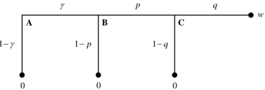
(7) has to deal with three consecutive bets. The first is on the existence of the unidentified species capable of supplying medicinal substances; the second is on the survival of such a species given its ambiguous survival; and the third is of whether the agent willing to fund the species protection will ever benefit from medical treatment in her lifetime. Therefore, we consider three independent lotteries A, B and C which respond to the three following questions: - Does the species exist? Lottery A - Will the species survive? Lottery B - Will the species be of use rapidly enough? Lottery C. . p. q. w B. A 1 . C. 1 p. 1 q. 0. 0. 0. Fig. 1 Three-stage lottery. We have a three-stage lottery of A : (B,  ;0,1   ) , B : (C, p;0,1  p) and C : (w, q; 0,1  q) . If the compound probability axiom holds, we can transform this multi-stage lottery into a reduced compound lottery D3 with a single stage (Figure 2) such as1 D3 : [w,  pq; 0,  p(1  q);0,  (1  p); 0,1   ]. (1). D3.  pq. 1 . w. 0.  p(1  q) 0 Fig. 2 Compound lottery. We ignore the case of  (1  p) on purpose. Indeed, contrary to  and q, the probability p of species survival depends on whether the agent decides to contribute to the public good. This bet is under her control. 1. 4.

(8) The probability of realization of the public good and thus the expected salvage of wealth amounts to. D3  (1   )(0)   p(1  q)(0)   pq(w)   pq(w)   (w) ,. (2). Where    pq . Nonetheless, the probability of existence and the probability of usefulness of the species do not affect its probability of survival, so the joint probability of survival given the other events is simply p. So ( p |  q)  p , and  ( w) reduces to p( w) . In other words, an agent who decides to act on the species survival and thus to affect its probability considers its existence and usefulness as granted. Otherwise, her reasoning has no sense. We consider the context of ambiguity by way of p [0,1] , because the probability of survival remains ambiguous after the agent contributed to the public good. The contributing agent ignores whether there is a free-rider, who might have jeopardized the threshold attainment and thus the probability of survival of the species, among all other agents in the population.. 3. Threshold public goods game. 3.1.Static game Let w  0 be the agent’s endowment or amount of wealth and g her contribution to the public good. To satisfy Nash equilibria, her contribution in the population of size N is bounded by the constraints of efficiency Ng  G and rationality g  w . The population is composed of contributors n and N  n free-riders. All agents must contribute their proportional fair-share. gk 1  Gk 1 N 1  0 to attain the threshold. The proportional fair-share is a fair-share in view of the spread of disease k [0,1] in the population. The proportional threshold then amounts to Gk 1  Ngk 1 . By means of prevalence proportion, we know that the probability of an agent, randomly picked from the population, of being at risk is equal to the proportion of the population which is at risk. When k  1 , the whole population is at risk of suffering from a disease, so the proportional fair-share equals GN 1 . As k  0 , the proportion of the population at risk rarefies and it is more and more costly for an agent to fund the public good. 5.

(9) Now consider the following expected payoff matrix.. Contributor. Free-rider. Contributor. p(w  gk 1 ) ; p(w  gk 1 ). (1  p)(w  gk 1 ) ; (1  p) w. Free-rider. (1  p) w ; (1  p)(w  gk 1 ). (1  p) w ; (1  p) w. If all agents contribute their proportional fair-share, we have n  N . The threshold is attained and the survival becomes certain p  1 . In this case, the analysis ceases, since the purpose of collective contributing is to increase the probability of survival of the species. Some agents may free-ride. In this case, we have ng  G  n(G / N )  G  0  N  n . The probability of survival is then ambiguous. The payoffs of a contributor and a free-rider are.   c  (1  p)( w  gk 1 )  p( w  gk 1 ) .   f  (1  p) w. (3). If there is a free-rider, the threshold cannot be attained. The probability that a contributor salvages her wealth given her contribution is p, and 1  p that she does not in presence of a free-rider. An agent who free-rides runs a risk of 1  p to fail savaging her wealth, not without reminding that she compromises p for every other contributing agent in the population. Simulations of g given p and k are presented in Table A.. 3.1.1. Null survival When the survival of species, i.e. probability of realization of the public good, is null or p  0 (3) reduces to 1   c  w  gk .   f  w. (4). We see that w  w  gk 1 . Free-riding always dominates because it provides a higher expected payoff.. 6.

(10) Proposition 1. In case of null survival of the species, free-riding always dominates.. 3.1.2. Ambiguous survival When the survival of species is ambiguous or p [0,1] , the outcome depends on the tradeoff between the proportional fair-share and the salvage of wealth in expectation. Two outcomes arise. If  c   f , we have gk 1  pw , so free-riding dominates because the proportional fairshare is greater than the expected benefit from contributing or the expected salvage of wealth. If  c   f , we have gk 1  pw , so contributing dominates because the cost of contributing to the public good is less than the expected benefit obtained from its production.. Proposition 2. In case of ambiguous survival of the species, contributing dominates when the proportional fair-share is less than the expected salvage of wealth. Otherwise, the agent is better off free-riding. Let us now linger on the k parameter. When the risk is high or k  1 , the trade-off. gk 1. pw reduces to g. pw and now depends on the fair-share level compared to the. expected salvage of wealth. As k  0 , the constraint against contributing gets unbounded or. limk 0 gk 1   , whereas pw  w . The trade-off is constrained by the endowment level, whereas low k provokes a proportional cost of contributing beyond the expected salvage of wealth. Thenceforth, when the probability of being at risk is low, the proportional fair-share exceeds the expected level of wealth, i.e. gk 1  pw . The fair-share stands out insufficient which induces collective underfunding of the public good.. Proposition 3. Low k provokes social underprovision and disinterest in the public good.. This result is consistent with the dead-anyway effect (Pratt and Zeckhauser, 1996), which states that willingness-to-pay increases with the level of risk to which the agent is exposed. The effect can be important in magnitude when the risk tends to one (Treich 2010).. 3.2. Dynamic game. 7.

(11) Following the work by Wang et al. (2009), we now combine game theory and population dynamics in a replicator equation. We consider infinite populations consisting of x contributors and y free-riders, where x  y  1, that is, the sum denotes a normalized population density such that 0 corresponds to a null population density and 1 is the maximal population density. According to replicator dynamics (Hofbauer and Sigmund 1998) the evolution of the system is given by the following differential equations.  x  x( f c  f ) ,  y  y ( f  f )  f. (5). The system in (5) establishes the expected payoffs of contributors f c and free-riders f f in time, given the average expected payoff in the population f  xf c  yf f . This payoff is determined by the interactions in randomly formed groups of contributors and free-riders. The groups are formed by interpreting densities as probabilities for drawing either strategy. We study the interactions of model-agents or average agents issued from those random groups. Let us set a mixed population where N agents are randomly chosen according to the Binomial probability function. Following Bailey et al. (2005), Hauert et al. (2006) and Wang et al. (2009), the probability that there are n contributors among the N  1 other agents in the population of size N in which the model-contributor or model-free-rider finds herself is determined by.  . f (n | N  1, x)  N  1 x n y N 1n . n. (6). This probability is independent of whether the model-agent is a contributor or a free-rider. Every model-agent encounters the same expected number of contributors, and hence the same expected payoff from others during the game. The only determinant of success in the wellmixed populations is the payoff that the model-agent herself receives. The expected payoffs of a model-contributor and a model-free-rider are.  f c  (1  p)( w  gk 1 )  p( w  gk 1 ) x N 1 ,  N 1  f f  (1  p) w(1  x ) 8. (7).

(12) where x N 1 and 1  x N 1 are the random variables that the model-agent issued from the Binomial distribution is respectively a contributor and a free-rider. Agents adopt the strategy of the model-agent with a probability proportional to the difference between her payoff and their own. Substituting y  1  x into the differential equations yields a single differential equation. x  x(1  x)( f c  f f ) ,. (8). So the dynamic evolution of x(t ) amounts to. x  x(1  x)[ p(w  gk 1 ) x N 1  (1  p)(w  gk 1 )  (1  p)w  (1  p)wx N 1 ] .. (9). 3.2.1. Null survival When the survival of species is null or p  0 , we obtain. x   x(1  x)(wx N 1  gk 1 ) .. (10). Solving x  0 gives two fixed points of the replicator dynamics which cancel out x(1  x) : x  0 and x  1 . We now proceed to the study of stability of steady states by the Lyapunov. method. The derivative of F ( x) is. F ( x)  (1  2 x)(wx N 1  gk 1 )  x(1  x)( N 1)wx N 2 .. (11). At x  0 , F (0)  0 , that is, a stable equilibrium. Since x  0  F (0) x if x  0 , a deviation brings x back to 0. At x  1 , F (1). 0 . If w  gk 1 , F (1)  0 . On the contrary, if w  gk 1 ,. F (1)  0 (Table 1). In the latter case, a deviation removes x from 1 and every agent freerides. Figure 3 illustrates the dynamics with null survival.. 9.

(13) Proposition 4. In case of null survival of the species, contributing is in steady state if the proportional fair-share is less than the level of wealth. Otherwise, the model-agent is better off free-riding. Let us now prospect the interior equilibrium. We reduce x(t ) to the function T ( x)  f c  f f. T ( x)  wx N 1  gk 1 .. (12). The interior equilibrium is the root of T ( x) in the interval [0,1] . Thus w  gk 1 , and T (1)  0 so there is no interior equilibrium. At T (0) , p [0,1] verifies T (0)  0 . Up to now, the fulfilled conditions are necessary but not sufficient. At last, we have. T ( x)  ( N  1)wx N 2 .. (13). T ( x)  0 is increasing which ends the proof. There is a unique root of T ( x)  0 situated in. [0,1] and it equals. x*  N 1. gk 1 . w. (14). At x  x * , T ( x*)  0 , that is, an unstable equilibrium (Table 1). Table 1 Stability of equilibria for p  0. gk 1  w. gk 1  w. x0. stable. [●]. x  x*. unstable. [○]. stable. [●]. x 1. unstable. [○]. Proposition 5. In case of null survival of the species, there is a unique unstable Nash equilibrium x * where the trade-off between the proportional fair-share and the level of wealth determines whether the model-agent ends up contributing or free-riding. 10.

(14) 1. x*. y. 0. x. 1. Fig. 3 Dynamics of x and y for p  0 .. Species being unlikely to survive or their risk of extinction is certain, agents suffer from their shortfall of survival. Regardless of the null probability of survival, agents will free-ride only if the cost of contributing exceeds their endowment constraint. In other words, agents continue to contribute with respect to their rationality constraint. This result appears counterintuitive, but can be explained by means of two behavioral concepts. The first is known as the illusion of control (Langer 1975), which is the penchant to overestimate the ability to control events. It here resumes to the collective illusion of control and manipulation of p. The second is the human tendency to act irrationally in despair (Buss 2004). By reason of the detrimental consequences of species extinction on biomedical finds and expected cures, agents at risk are willing to attempt anything and still contribute to the public good.. 3.2.2. Ambiguous survival When the survival of species is ambiguous or 0  p  1 , we have. x  x(1  x)[ p(w  gk 1 ) x N 1  (1  p)(w  gk 1 )  (1  p)w  (1  p)wx N 1 ] .. (15). Fixing x  0 gives two fixed points of the replicator dynamics: x  0 and x  1 . We look at the derivative of F ( x) which is. F ( x)  (1  2 x)[ p( w  gk 1 ) x N 1  (1  p)( w  gk 1 )  (1  p) w  (1  p) wx N 1 ]  x(1  x)[( N  1) wx N 2  ( N  1) pgk 1 x N 2 ]. 11. .. (16).

(15) At x  0 , F (0)  0 , that is, a stable equilibrium. At x  1 , F (1). 0 . Just as with the case of. null survival, if w  gk 1 , F (1)  0 which implies a steady state. If w  gk 1 , the equilibrium is unstable (Table 2).. Proposition 6. In case of ambiguous survival of the species, contributing is in steady state if the proportional fair-share is less than the level of wealth. Otherwise, the model-agent is better off free-riding. Let us now prospect the interior equilibrium. We reduce x(t ) to the function T ( x)  f c  f f. T ( x)  p(w  gk 1 ) x N 1  (1  p)(w  gk 1 )  (1  p)w  (1  p)wx N 1 .. (17). We have T (0)  0 and T (1)  0 . At last, we have. T ( x)  ( N  1)(w  pgk 1 ) x N 2 .. (18). Given the rationality constraint, T ( x)  0 . The root of T ( x)  0 equals. x* . N 1. gk 1  pgk 1 . w  pgk 1. (19). At x  x * , T ( x*)  0 , that is, an unstable equilibrium (Table 2). Figures 4 and 5 show the ambiguous survival dynamics. Simulations of g at x * are presented in Table B. Table 2 Stability of equilibria for p  [0,1]. gk 1  w. gk 1  w. x0. stable. [●]. x  x*. unstable. [○]. stable. [●]. x 1. unstable. [○]. 12.

(16) 1. 1. y. y. 0. x*. x. 1. x. 0. Fig. 4 Dynamics of x and y for p  [0,1] and gk 1  w. 1. Fig. 5 Dynamics of x and y for p  [0,1] and gk 1  w. Proposition 7. In case of ambiguous survival of the species, there is a unique unstable Nash equilibrium x * where the trade-off between the proportional fair-share and the level of wealth determines whether the model-agent ends up contributing or free-riding.. Despite the ambiguous survival of species and hence the ambiguous benefits from the species conservancy, agents will contribute with respect to their rationality constraint. Once again, the agents’ illusion of being fully in control of the ecosystems in the face of uncertainty, ignorance and risk (Frissell and Bayles 1996) explains our results. When the risk is high or k  1 , the trade-off gk 1. w depends on the level of. wealth. As the risk turns low or k  0 , the constraint against contributing gets unbounded or. limk 0 gk 1   . In parallel, we have w   . Thenceforth, when the risk is low, the proportional fair-share exceeds the level of wealth. We have gk 1  w . This result invalidates the argument defended by Olson (1968) and Marwell and Ames (1979) who state that public goods are provided by groups in which an individual has an interest in the good that is greater than the cost of the good. The high interest of an agent at risk does not suffice to cover the cost of the public good. The only case where their argument could hold water is if the model-agent is the agent at stake.. 4. Public goods option market game. 4.1.Static game. Now consider an option market for the public good, where agents exchange option contracts on public goods by buying and selling until the market price is settled. The option market 13.

(17) price can reveal the social probability of species survival and of the attainment of the threshold. We assume the market-efficiency hypothesis. For that reason, the threshold can only be attained at the market equilibrium where all possible exchanges are cleared at the market price. The market then equally splits between buyers and sellers. In this case, the proportional fair-share equals the expected payoff from salvaging wealth at the market price. Because exchanges are based upon predictions of the probability of species survival, our option market is a prediction market. The prediction market can be considered a representative person with a set of expectations (Wolfers and Zitzewitz 2004). Even though the equilibrium price does not reveal the mean belief that agents hold, it yields a bound on the mean belief (Manski 2006). The equilibrium reveals the position of the model-agent. The agent is defined a buyer if she believes that p  0.5 , and a seller otherwise. Yet, there is a difference between the standard prediction market and ours. The latter does not produce outcomes tied to events exogenous to the market. Indeed, option exercises depend on the number of betting exchanges cleared on the market. If agents conclude an insufficient number of option contracts, they fail to sufficiently provide the public good and the species survival is jeopardized. In turn, buyers fall salvaging their wealth through, and sellers lose their premium from bearing the risk of species extinction.. In terms of the expected payoff matrix, we have. Buyer. Seller. Buyer. (1  p)(w  gk 1 ) ; (1  p)(w  gk 1 ). p(w  gk 1 ) ; (1  p)w  p. Seller. (1  p)w  p ; p(w  gk 1 ). (1  p) w ; (1  p) w. Buyers willing to increase the species probability of survival offer to buy option contracts at their willingness-to-pay, i.e. their proportional fair-share, whereas sellers unconvinced of the survival likelihood propose selling contracts at their willingness-to-accept. If a buyer happens to meet a buyer, their contracts are not exchanged and both face the risk of 1  p of losing their wealth. Likewise, if both agents propose asks, they are exposed by 1  p to the wealth disappearance. Otherwise, the buyer salvages her wealth at p by bidding her proportional fairshare and the seller receives a premium of p for her asking price, which here corresponds to the option price: the survival probability times the offer.. 14.

(18) The market of size M is divided between m buyers and M  m sellers. If all the bidask. spreads. are. zero. and. buyers’. and. sellers’. bids. and. offers. match. or. m  M  m  m  M / 2 , the option market is fully efficient and the threshold is attained. If m  M  m and m  M / 2 , the payoffs of a buyer and a seller facing an ambiguous. probability of species survival are 1 1   b  (1  p)( w  gk )  p( w  gk ) .    s  (1  p) w  p. (17). 4.1.1. Null survival When the survival of species is null or p  0 , (17) reduces to.  b  w  gk 1  .    s  w. (18). We have w  w  gk 1 . Selling the option contract of the species survival provides a higher expected payoff so traders are net sellers.. Proposition 8. In case of null survival of the species, selling option contracts always dominates.. 4.1.2. Ambiguous survival When p [0,1] , the outcome depends on the tradeoff between the proportional fair-share and the expected salvage of wealth at the market price. We have two possible outcomes. If.  b   s then gk 1  p(w   ) , that is, the cost of contributing is greater than the expected payoff from salvaging wealth at the market price; the option price is greater than the expected payoff from contributing, so agents are net sellers. If  b   s we have gk 1  p(w   ) . The expected payoff from contributing is less than the expected benefit from salvaging wealth at the market price so agents are net buyers. Finally, at p  pw  gk 1 , buyers and sellers. 15.

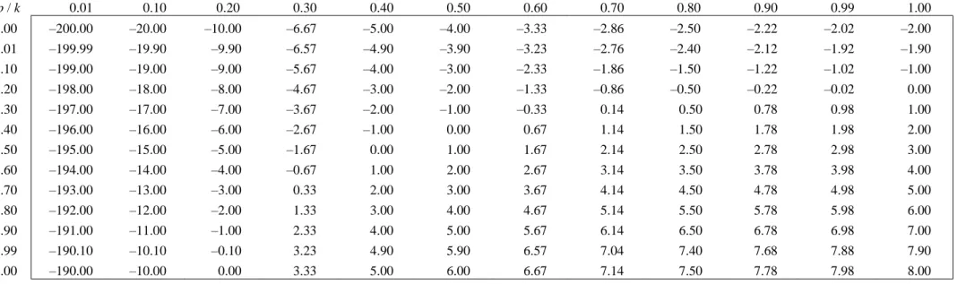
(19) equalize their payoffs or  b   s and the market is fully efficient. Therefore, the public good will be provided by the option market for p  gk 1 (w   )1 .. Proposition 9. In case of ambiguous survival of the species, agents exchanging option contracts at the market equilibrium equally split between buyers and sellers for. p  gk 1 (w   )1 . Otherwise, either buying or selling option contracts dominates.. Simulations in Table C show that for levels of k and p close to zero, the unbounded constraint against contributing yields negative option prices. The risk premium turns out to be negative. Despite appearances, this result is not absurd, and is known to exist in the capital asset pricing model. Analyzing premiums for public good losses resumes to studying the agents’ behavior in a context where property rights are passed over. In our case, the agent has to consider herself the owner of the public good from which she loses her wealth. Asking for compensation demanded for the public loss, even in case of private fatalities, makes de facto selling agents creditors of the public good. And we know, for example, that risk premium can be negative with credit default option swap contracts. As a result, when agents decide to sell an option contract on the public good, the option price reveals that they ask the market to protect them from their potential loss of wealth in exchange of a premium. Buyers of option contracts become the sellers of the protection contracts they demand. Since scarcity is highly valued on markets, the rarer the disease is, the higher the premium gets. As a result, the cost of protecting oneself on an option market, given the smallness of k, is exorbitant. On the contrary, when k and p tend to 1, option prices are close to the level of wealth: buyers’ expected benefit from providing the public good approximates their proportional fairshare. Therefore, the option market fails to be surplus-generating. The game is solved with public demand and supply which never meet. Given that no buyer will accept to contribute unless her benefit from the public good overpasses her cost of funding it, and given that no seller will accept to exchange at a negative price unless she asks the market to protect her from the risk of wealth loss, only a non-market provision at a fiscal capitation relative to the society’s risk aversion seems feasible. Although the option market mechanism can be efficient enough to equalize expected benefits and costs and thus to produce the public good, it produces null surpluses at the equilibrium and thus fails to fulfill the role it has been assigned.. 16.

(20) Proposition 10. Low k and/or low p induce negative option prices, i.e. sellers of the option contract demand protection for the probable loss. High k and p induce quasi-null option prices, i.e. buyers’ expected payoff at the market price equals their proportional fair-share. The results imply the absence of surplus captured on the option market.. 4.2. Dynamic game We now consider infinite populations of x buyers and y sellers, where x  y  1 . Let z  x / y denote the ratio of buyers to sellers. The evolution of the system is given by the following differential equations.   z  z ( fb  f ) ,   1  z  (1  z )( f s  f ). (19). where z and 1  z establish the market surpluses of the demand f b and supply f s sides, given the average surplus in the market f  zfb  (1  z ) f s . Let us set a mixed population where M agents are randomly chosen. In large markets, the probability that a buyer faces m buyers in the population of size M at a particular seller is given by the Binomial distribution. . . f (m | M  1, z )  M  1 z m (1  z ) M 1m . m. (20). In the population, the probability for a model-buyer to be allocated the exchange is (m  1)1 . Indeed, the model-seller chooses a model-buyer at random when more than one. Following the work of Bach et al. (2006) and Julien et al. (2008), the probability for a buyer to be served when selecting a seller is given by. [1  (1  z) M ]( Mz)1 .. (21). (1  z ) M is the probability that model-agents do not match, i.e. all the surplus is captured by the supply side, so [1  (1  z) M ]( Mz)1 is the probability that the model-buyer finds the right model-seller, given the agents available on the market. The probability that the model-seller 17.

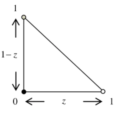
(21) sells an option contract is [1  (1  z ) M ] . The average payoffs of a model-buyer and a modelseller become 1 1 M 1   fb  (1  p)( w  gk )  p(w  gk )[1  (1  z ) ](Mz ) .  M   f s  (1  p) w  p [1  (1  z ) ]. (22). The differential equations yield a single formulation in form of. z  z (1  z )( fb  f s ) ,. (23). So the dynamic evolution of z (t ) amounts to. z  z(1  z)[ p [(w  gk 1 )[1  (1  z) M ](Mz)1   [1  (1  z) M ]]  (1  p) gk 1 ] .. (24). 4.2.1. Null survival When the survival of species is null or p  0 , we obtain. z   z (1  z ) gk 1 .. (25). Solving z  0 gives two fixed points of the replicator dynamics which cancel out z (1  z ) :. z  0 and z  1. The derivative of F ( z ) is F ( z)   gk 1  2 zgk 1 .. (26). At z  0 , F (0)  0 , that is, a stable equilibrium. At z  1 , F (1)  0 , which implies an unstable equilibrium (Table 3). Figure 6 points up the dynamics.. 18.

(22) 1. 1 z. 0. z. 1. Fig. 6 Dynamics of z and 1  z for p  0. Proposition 11. In case of null survival of the species, sellers of option contracts are in steady state and the public good fails to be provided. Table 3 Stability of equilibria for p  0. z0. stable. [●]. z 1. unstable. [○]. 4.2.2. Ambiguous survival When the survival of species is ambiguous or 0  p  1 , we have. z  z(1  z)[ p [(w  gk 1 )[1  (1  z) M ](Mz)1   [1  (1  z) M ]]  (1  p) gk 1 ] .. (27). Fixing z  0 gives two fixed points: z  0 and z  1 . The derivative of F ( z ) is. F ( z )  (1  2 z )[ p [( w  gk 1 )[1  (1  z ) M ]( Mz ) 1   [1  (1  z ) M ]]  (1  p) gk 1 ]  z (1  z )[ p [ z 2 [ z (1  z ) M 1  [(1  z ) M  1]M 1 ](w  gk 1 )  M (1  z ) M 1 ]] At z  0 , F (0)  0 , that is, a stable equilibrium. At z  1 , F (1). .. (28). 0 . If the inequality. gk 1  p(wM 1   )[ p(1  M )M 1  1]1 is verified, F (1)  0 and we are in presence of a steady state. If gk 1  p(wM 1   )[ p(1  M )M 1  1]1 the equilibrium is unstable (Table 4). The expression p(1  M )M 1  1 corresponds to the market liquidity, that is, the opportunity. 19.

(23) to complete the transaction without significant movements in the market price. Simulations of. p are presented in Table D.. Proposition 12. In case of ambiguous survival of the species, agents exchanging option contracts at the market equilibrium are in steady state if, given the market liquidity, the proportional fair-share is less than the expected salvage of wealth.. However, to verify the inequality of inferiority of the steady state, the option price must be close to zero, that is, sellers sell option contracts to buyers for free. Therefore, this result is highly unlikely. We then reduce z (t ) to the function S ( z )  fb  f s. S ( z)  p [(w  gk 1 )[1  (1  z)M ](Mz)1   [1  (1  z)M ]]  (1  p) gk 1 .. (29). The interior equilibrium has a root of S ( z ) in [0,1] . We have z  0 or S (0)  0 . In parallel, at. z  1, S (1)  0 if gk 1  p(wM 1   )[ p(1  M )M 1  1] , and S (1)  0 if inferior. Derivation yields. S ( z)  p [ z 2 [ z(1  z)M 1  [(1  z) M 1] M 1 ](w  gk 1 )  M (1  z) M 1 ] .. (30). Given that lim z 1 z 2 [ z(1  z) M 1  [(1  z) M 1] M 1 ]  0 and lim z 1 M (1  z) M 1  0 we have. S ( z )  0 when gk 1  w(0 / 0 )   (0 / 0 ) which is always verified. Given that M  0 and z  0 , S ( Z )  0 reduces to. p( w   )  gk 1 . (1  z )  p( w   )  pgk 1 M. (31). By substituting (1  z ) with Z, the root of S (Z )  0 is a complex number equal to Re[M ]  0 , Z *  0 .. 20. (32).

(24) At Z *  0 , S (Z *)  0 and the equilibrium is stable (Table 4). Since Z *  (1  z )* , we have. z  1 or x / y  1 which implies that x  y . Figures 7 and 8 illustrate the dynamics depending on the trade-off rule. At z  1 , we have gk 1  pgk 1 or p  1 . Simulations of p at the equilibrium are presented in Table E.. Proposition 13. There is a unique stable Nash equilibrium z * where agents exchanging option contracts at the market equilibrium are in steady state if, given the market liquidity, the proportional fair-share is greater than the expected salvage of wealth. The market is then fully efficient or x. y and the public good is provided. This result holds only for p  1 .. Table 4 Stability of equilibria for. gk 1 . p ( wM 1  ) p (1 M ) M 1 1. z0. stable. [●]. z  z*. stable. [●]. z 1. unstable. [○]. p [0,1]. gk 1 . p ( wM 1  ) p (1 M ) M 1 1. stable. [●]. stable. [●]. 1. 1. 1 z. 1 z. 0. z. 0. 1. Fig. 7 Dynamics of z and 1  z for 1. p  [0,1] and gk . z*. z. 1. Fig. 8 Dynamics of z and 1  z for. p ( wM 1  ). p  [0,1] and gk 1 . p (1 M ) M 1 1. p ( wM 1  ) p (1 M ) M 1 1. Both low and high levels of k yield low negative or quasi-null option prices. Low negative option prices reveal that the proportional fair-share is to some extent greater than the salvage of wealth at the market price. Quasi-null option prices imply that the payoff from salvaging wealth at the market price equals the proportional fair-share. The null option price result is consistent with Plummer (1986) who shows that if the project attainment fails to change the probability of supply of the public good (and thus remains ambiguous), option price is zero. 21.

(25) Market prices close to zero reflect the fact that model-agents only exchange for p  1 . Therefore, buyers and sellers will withdraw from the option market, because they do not expect a higher benefit from the public good than the cost of funding it. Given that no surplus is captured at the equilibrium, the option market will remain inert and therefore collapse.. 5. Conclusion. Our static threshold public goods game first reveals that agents free-ride in case of null survival of the species. Then, the game shows coexistence of free-riders and contributors in case of ambiguous survival of the species. Agents contribute if their proportional fair-share is less than their expected salvage of wealth. From the cost-benefit analysis, it simply states that agents are willing to contribute to the public good if their expected benefit from the public good exceeds the cost of producing it. Our dynamic threshold public goods game shows that contributing is in steady state if the proportional fair-share is less than the level of wealth, be it within null or ambiguous survivals of the species. We can notice that the expectation over the level of wealth disappears in the dynamic analysis where the rationality constraint accounts only. The result appears to be consistent with Bernheim (1984) who shows that dynamic rationality imposes restrictions that lead to boundedly rational behaviors. Given the infinite time length in dynamic settings, it is understandable that agents will abstain from making expectations on their outcomes. As a final point, we find that in case of rare diseases, social free-riding is unavoidable. Ultimately, the results of our games show that agents tend to contribute to the public good in ambiguity, as long as they bear the risk of suffering personal losses. The result is conforming to the results by Bailey et al. (2005), who find less free-riding in ambiguity in presence of large populations. As regards the static option market for public goods, when the probability of survival of the species is zero, agents are net sellers. When the probability is ambiguous, the market is fully efficient, i.e. the public good is provided, only if the proportional fair-share is equal to the expected payoff from salvaging wealth at the market price. This result holds for a specific market belief over the species survival. Sellers face negative option prices, meaning that they are in demand for protection for running the probable loss of wealth. On the demand side of the market, option market prices are close to zero, signifying that the expected payoff from salvaging wealth at the market price equals the proportional fair-share. Provided the absence of surplus realized on the market, agents have no incentive to exchange contracts. The option market is doomed to disappear, which condemns the species survival. The results from the 22.

(26) dynamic public goods option market game are similar, except that the market efficiency occurs when the market belief over the species survival is one. This explains why most market prices are quasi-null at the equilibrium. Henceforth, the mainspring for the option market no longer runs. In all cases, providing ambiguous environmental public goods by option markets is socially inefficient.. References Acton, J. (1973), “Evaluating Public Programs to Save Lives: The Case of Heart Attacks”, R950-RC, RAND, Santa Monica. Arrow, K. and Fisher, A. (1974), “Environmental Preservation, Uncertainty, and Irreversibility”, Quarterly Journal of Economics, 88: 312–319. Arrow, K., Forsythe, R., Gorham, M., Hahn, R., Hanson, R., Ledyard, J., Levmore, S., Litan, R., Milgrom, P., Nelson, F., Neumann, G., Ottaviani, M., Schelling, T., Shiller, R., Smith, V., Snowberg, E., Sunstein, C., Tetlock, P. and Tetlock, P. (2008), “The Promise of Prediction Markets”, Science, 320: 877–878. Au, W. (2004), “Criticality and Environmental Uncertainty in Step-Level Public Goods Dilemmas”, Group Dynamics: Theory, Research and Practice, 8: 40–61. Bach, L., Helvik, T. and Christiansen, F. (2006), “The Evolution of N-Player CooperationThreshold Games and ESS Bifurcations”, Journal of Theoretical Biology, 238: 426– 434. Bailey, R., Eichberger, J. and Kelsey, D. (2005), “Ambiguity and Public Good Provision in Large Societies”, Journal of Public Economic Theory, 7: 741–759. Berg, J., Forsythe, R., Nelson, F. and Rietz, T. (2008), “Results from a Dozen Years of Election Futures Markets Research,” in Handbook of Experimental Economic Results, Charles Plott and Vernon Smith, eds. Amsterdam, Elsevier. Bernheim, D. (1984), “Rationalizable Strategic Behavior”, Econometrica, 52: 1007–1028. Buss, S. (2004), “The Irrationality of Unhappiness and the Paradox of Despair”, Journal of Philosophy, 101: 167–196. Chivian, E. and Bernstein, A. (2004), “Embedded in Nature: Human Health and Biodiversity”, Environmental Health Perspectives, 112: 12–13. Dreber, A. and Nowak, M. (2008), “Gambling for Global Goods”, Proceedings of the National Academy of Sciences of the United States of America, 105: 2261–2262. Forsythe, R., Rietz, T. and Ross, T. (1999), “Wishes, Expectations and Actions: Price Formation in Election Stock Markets”, Journal of Economic Behavior and Organization, 39: 83–110. Frissell, C. and Bayles, D. (1996), “Ecosystem Management and the Conservation of Aquatic Biodiversity and Ecological Integrity”, Water Resources Bulletin, 32: 229–240. Gangadharan, L. and Nemes, V. (2009), “Experimental Analysis of Risk and Uncertainty in Provisioning Private and Public Goods”, Economic Inquiry, 47: 146–164. Hammitt, J. and Graham, J. (1999), “Willingness to Pay for Health Protection: Inadequate Sensitivity to Probability”, Journal of Risk and Uncertainty, 8: 33–62. Hauert, C., Holmes, M., and Doebeli, M. (2006), “Evolutionary Games and Population Dynamics: Maintenance of Cooperation in Public Goods Games”, Proceedings of the Royal Society B, 273: 2565–2570. Hofbauer, J., and Sigmund, K. (1998), “Evolutionary Games and Population Dynamics”, Cambridge University Press. 23.

(27) Jones-Lee, M., Hammerton, M. and Philips, P. (1985), “The Value of Safety: Results of a National Survey”, Economic Journal, 95: 49–72. Julien, B., Kennes, J. and King, I. (2008), “Bidding for Money”, Journal of Economic Theory, 142: 196–217. Langer, E. (1975), “The Illusion of Control”, Journal of Personality and Social Psychology, 32: 311–328. Link, A. and Scott, J. (2005), “Evaluating Public Research Institutions: The U.S. Advanced Technology Program’s Intramural Research Initiative”, London: Routledge. Manski, C. (2006), “Interpreting the Predictions of Predictions Markets”, Economics Letters, 91: 425–429. Marwell, G. and Ames, R. (1979), “Experiments on the Provision of Public Goods. I. Resources, Interest, Group Size, and the Free-Rider Problem”, American Journal of Sociology, 84: 1335– 1360. McBride, M. (2006), “Discrete Public Goods under Threshold Uncertainty”, Journal of Public Economics, 90: 1181–1199. Milinski, M., Sommerfeld, R., Krambeck, H-J., Reed, F. and Marotzke, J. (2008), “The Collective-Risk Social Dilemma and the Prevention of Stimulated Dangerous Climate Change”, Proceedings of the National Academy of Sciences of the United States of America, 105: 2291–2294. Olson, M. (1968), “The Logic of Collective Action: Public Goods and the Theory of Groups”, New York: Schocken. Plummer, M. (1986), “Supply Uncertainty, Option Price, and Option Value: An Extension”, Land Economics, 62: 313–318. Polasky, S. and Solow, A. (1995), “On the Value of a Collection of Species”, Journal of Environmental Economics and Management, 29: 298–303. Pratt, J. and Zeckhauser, R. (1996), “Willingness to Pay and the Distribution of Risk and Wealth”, Journal of Political Economy, 104: 747–763. Schelling, T. (1992), “Some Economics of Global Warming”, American Economic Review, 82: 1–14. Suleiman, R. (1997), “Provision of Step-Level Public Goods under Uncertainty: A Theoretical Analysis”, Rationality and Society, 9: 163–187. Thomas, C., Cameron, A., Green, R., Bakkenes, M., Beaumont, L., Collingham, Y., Erasmus, B., Ferreira de Siqueira, M., Grainger, A., Hannah, L., Hughes, L., Huntley, B., van Jaarsveld, A., Midgley, G., Miles, L., Ortega-Huerta, M., Peterson, A., Philips, O. and Williams, S. (2004), “Extinction Risk from Climate Change”, Nature, 427: 145–148. Thompson, M., Read, J. and Liang, M. (1984), “Feasibility of Willingness-to-Pay Measurement in Chronic Arthritis”, Medical Decision Making, 4: 195–215. Treich, N. (2010), “The Value of a Statistical Life under Ambiguity Aversion”, Journal of Environmental Economics and Management, 59: 15–26. Viscusi, K., Magat, W. and Huber, J. (1987), “An Investigation of the Rationality of Consumer Valuations of Multiple Health Risks”, RAND Journal of Economics, 18: 465–479. Wang, J., Fu, F., Wu, T. and Wang, L. (2009), “Emergence of Social Cooperation in Threshold Public Goods Games with Collective Risk”, Physical Review, 80: 016101.1–016101.11. Wang, J., Fu, F. and Wang, L. (2010), “Effects of Heterogeneous Wealth Distribution on Public Cooperation with Collective Risk”, Physical Review, 82: 016102.1–016102.13. Weinstein, M., Shepard, D. and Pliskin, J. (1980), “The Economic Value of Changing Mortality Probabilities: A Decision-Theoretic Approach”, Quarterly Journal of Economics 94: 373–96. 24.

(28) Weitzman, M. (1998), “The Noah’s Ark Problem”, Econometrica, 66: 1279–1298. Wit, A. and Wilke, H. (1998), “Public Good Provision under Environmental and Social Uncertainty”, European Journal of Social Psychology, 28: 249–256. Wolfers, J. and Zitzewitz, E. (2004), “Prediction Markets”, Journal of Economic Perspectives, 18: 107–126. Wright, J. and Muller-Landau, H. (2006), “The Uncertain Future of Tropical Forest Species”, Biotropica, 38: 443–445.. Appendix.  . Equation (7): we know from the Binomial theorem that nN01 N  1 x n (1  x) N 1n  1 , thus n. Pr ( N  1  n)  x N 1 .. . . Equation (21). From the Binomial sampling, we have mM01 (m  1)1 M  1 z m (1  z ) M 1m m.  mM11 M 1.  mM1 z (1 z) m. M 1 m.  .  ( Mz )1  mM0 M z m (1  z ) M m  and [1  (1  z) M ]( Mz)1 . m  . 25.

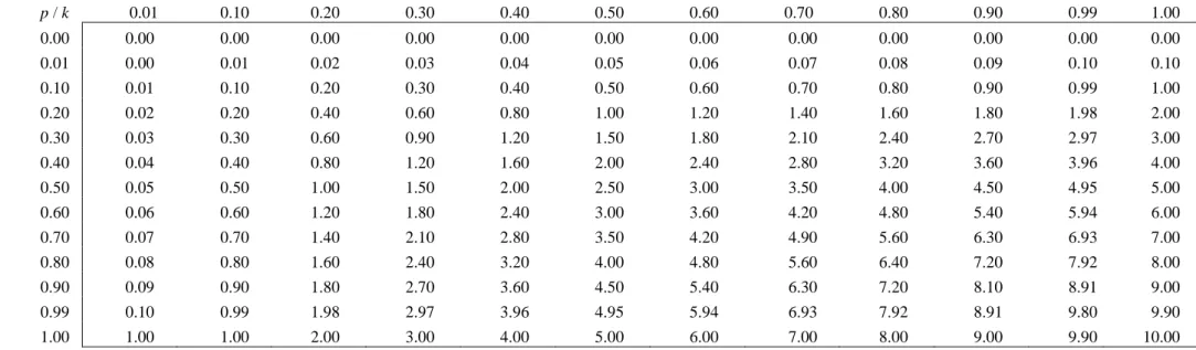
(29) Table A Simulations in dollars of the contributor’s static fair-share g given p and k for w  10 : g  pwk. p/k. 0.01. 0.10. 0.20. 0.30. 0.40. 0.50. 0.60. 0.70. 0.80. 0.90. 0.99. 1.00. 0.00. 0.00. 0.00. 0.00. 0.00. 0.00. 0.00. 0.00. 0.00. 0.00. 0.00. 0.00. 0.00. 0.01. 0.00. 0.01. 0.02. 0.03. 0.04. 0.05. 0.06. 0.07. 0.08. 0.09. 0.10. 0.10. 0.10. 0.01. 0.10. 0.20. 0.30. 0.40. 0.50. 0.60. 0.70. 0.80. 0.90. 0.99. 1.00. 0.20. 0.02. 0.20. 0.40. 0.60. 0.80. 1.00. 1.20. 1.40. 1.60. 1.80. 1.98. 2.00. 0.30. 0.03. 0.30. 0.60. 0.90. 1.20. 1.50. 1.80. 2.10. 2.40. 2.70. 2.97. 3.00. 0.40. 0.04. 0.40. 0.80. 1.20. 1.60. 2.00. 2.40. 2.80. 3.20. 3.60. 3.96. 4.00. 0.50. 0.05. 0.50. 1.00. 1.50. 2.00. 2.50. 3.00. 3.50. 4.00. 4.50. 4.95. 5.00. 0.60. 0.06. 0.60. 1.20. 1.80. 2.40. 3.00. 3.60. 4.20. 4.80. 5.40. 5.94. 6.00. 0.70. 0.07. 0.70. 1.40. 2.10. 2.80. 3.50. 4.20. 4.90. 5.60. 6.30. 6.93. 7.00. 0.80. 0.08. 0.80. 1.60. 2.40. 3.20. 4.00. 4.80. 5.60. 6.40. 7.20. 7.92. 8.00. 0.90. 0.09. 0.90. 1.80. 2.70. 3.60. 4.50. 5.40. 6.30. 7.20. 8.10. 8.91. 9.00. 0.99. 0.10. 0.99. 1.98. 2.97. 3.96. 4.95. 5.94. 6.93. 7.92. 8.91. 9.80. 9.90. 1.00. 1.00. 1.00. 2.00. 3.00. 4.00. 5.00. 6.00. 7.00. 8.00. 9.00. 9.90. 10.00. 26.

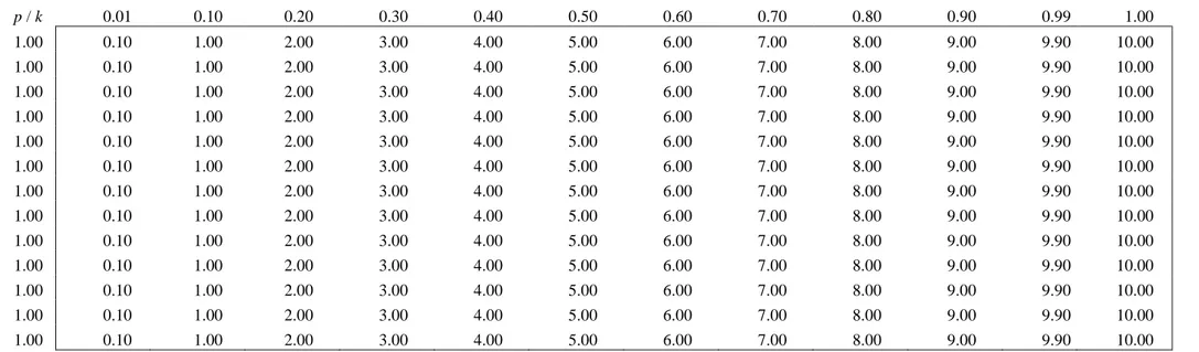
(30) Table B Simulations in dollars of the contributor’s dynamic fair-share g at the equilibrium ( x*  1 ) given k and w  10 : g  wk. p/k. 0.01. 0.10. 0.20. 0.30. 0.40. 0.50. 0.60. 0.70. 0.80. 0.90. 0.99. 1.00. 1.00. 0.10. 1.00. 2.00. 3.00. 4.00. 5.00. 6.00. 7.00. 8.00. 9.00. 9.90. 10.00. 1.00. 0.10. 1.00. 2.00. 3.00. 4.00. 5.00. 6.00. 7.00. 8.00. 9.00. 9.90. 10.00. 1.00. 0.10. 1.00. 2.00. 3.00. 4.00. 5.00. 6.00. 7.00. 8.00. 9.00. 9.90. 10.00. 1.00. 0.10. 1.00. 2.00. 3.00. 4.00. 5.00. 6.00. 7.00. 8.00. 9.00. 9.90. 10.00. 1.00. 0.10. 1.00. 2.00. 3.00. 4.00. 5.00. 6.00. 7.00. 8.00. 9.00. 9.90. 10.00. 1.00. 0.10. 1.00. 2.00. 3.00. 4.00. 5.00. 6.00. 7.00. 8.00. 9.00. 9.90. 10.00. 1.00. 0.10. 1.00. 2.00. 3.00. 4.00. 5.00. 6.00. 7.00. 8.00. 9.00. 9.90. 10.00. 1.00. 0.10. 1.00. 2.00. 3.00. 4.00. 5.00. 6.00. 7.00. 8.00. 9.00. 9.90. 10.00. 1.00. 0.10. 1.00. 2.00. 3.00. 4.00. 5.00. 6.00. 7.00. 8.00. 9.00. 9.90. 10.00. 1.00. 0.10. 1.00. 2.00. 3.00. 4.00. 5.00. 6.00. 7.00. 8.00. 9.00. 9.90. 10.00. 1.00. 0.10. 1.00. 2.00. 3.00. 4.00. 5.00. 6.00. 7.00. 8.00. 9.00. 9.90. 10.00. 1.00. 0.10. 1.00. 2.00. 3.00. 4.00. 5.00. 6.00. 7.00. 8.00. 9.00. 9.90. 10.00. 1.00. 0.10. 1.00. 2.00. 3.00. 4.00. 5.00. 6.00. 7.00. 8.00. 9.00. 9.90. 10.00. 27.

(31) Table C Simulations in dollars of static option prices p given p and k for w  100 : p  pw  gk 1. p/k. 0.01. 0.10. 0.20. 0.30. 0.40. 0.50. 0.60. 0.70. 0.80. 0.90. 0.99. 1.00. 0.00. –200.00. –20.00. –10.00. –6.67. –5.00. –4.00. –3.33. –2.86. –2.50. –2.22. –2.02. –2.00. 0.01. –199.99. –19.90. –9.90. –6.57. –4.90. –3.90. –3.23. –2.76. –2.40. –2.12. –1.92. –1.90. 0.10. –199.00. –19.00. –9.00. –5.67. –4.00. –3.00. –2.33. –1.86. –1.50. –1.22. –1.02. –1.00. 0.20. –198.00. –18.00. –8.00. –4.67. –3.00. –2.00. –1.33. –0.86. –0.50. –0.22. –0.02. 0.00. 0.30. –197.00. –17.00. –7.00. –3.67. –2.00. –1.00. –0.33. 0.14. 0.50. 0.78. 0.98. 1.00. 0.40. –196.00. –16.00. –6.00. –2.67. –1.00. 0.00. 0.67. 1.14. 1.50. 1.78. 1.98. 2.00. 0.50. –195.00. –15.00. –5.00. –1.67. 0.00. 1.00. 1.67. 2.14. 2.50. 2.78. 2.98. 3.00. 0.60. –194.00. –14.00. –4.00. –0.67. 1.00. 2.00. 2.67. 3.14. 3.50. 3.78. 3.98. 4.00. 0.70. –193.00. –13.00. –3.00. 0.33. 2.00. 3.00. 3.67. 4.14. 4.50. 4.78. 4.98. 5.00. 0.80. –192.00. –12.00. –2.00. 1.33. 3.00. 4.00. 4.67. 5.14. 5.50. 5.78. 5.98. 6.00. 0.90. –191.00. –11.00. –1.00. 2.33. 4.00. 5.00. 5.67. 6.14. 6.50. 6.78. 6.98. 7.00. 0.99. –190.10. –10.10. –0.10. 3.23. 4.90. 5.90. 6.57. 7.04. 7.40. 7.68. 7.88. 7.90. 1.00. –190.00. –10.00. 0.00. 3.33. 5.00. 6.00. 6.67. 7.14. 7.50. 7.78. 7.98. 8.00. 28.

(32) Table D Simulations in dollars of dynamic option prices p given p, k for w  10 and M  G  100 : p  pwM 1  gk 1[ p(1  M ) M 1  1]. p/k. 0.01. 0.10. 0.20. 0.30. 0.40. 0.50. 0.60. 0.70. 0.80. 0.90. 0.99. 1.00. 0.01. –198.02. –19.80. –9.90. –6.60. –4.95. –3.96. –3.30. –2.83. –2.47. –2.20. –2.00. –1.98. 0.10. –180.19. –18.01. –9.00. –6.00. –4.50. –3.59. –2.99. –2.56. –2.24. –1.99. –1.81. –1.79. 0.20. –160.38. –16.02. –8.00. –5.33. –3.99. –3.19. –2.65. –2.27. –1.99. –1.76. –1.60. –1.58. 0.30. –140.57. –14.03. –7.00. –4.66. –3.49. –2.78. –2.31. –1.98. –1.73. –1.53. –1.39. –1.38. 0.40. –120.76. –12.04. –6.00. –3.99. –2.98. –2.38. –1.97. –1.69. –1.47. –1.30. –1.18. –1.17. 0.50. –100.95. –10.05. –5.00. –3.32. –2.48. –1.97. –1.63. –1.39. –1.21. –1.07. –0.97. –0.96. 0.60. –81.14. –8.06. –4.00. –2.65. –1.97. –1.56. –1.29. –1.10. –0.96. –0.84. –0.76. –0.75. 0.70. –61.33. –6.07. –3.00. –1.98. –1.47. –1.16. –0.95. –0.81. –0.70. –0.61. –0.55. –0.54. 0.80. –41.52. –4.08. –2.00. –1.31. –0.96. –0.75. –0.61. –0.51. –0.44. –0.38. –0.34. –0.34. 0.90. –21.71. –2.09. –1.00. –0.64. –0.46. –0.35. –0.27. –0.22. –0.18. –0.15. –0.13. –0.13. 0.99. –3.88. –0.30. –0.10. –0.03. –0.00. 0.02. 0.03. 0.04. 0.05. 0.05. 0.06. 0.06. 1.00. –1.90. –0.10. 0.00. 0.03. 0.05. 0.06. 0.07. 0.07. 0.08. 0.08. 0.08. 0.08. 29.

(33) Table E Simulations in dollars of dynamic market prices at the equilibrium ( p  1 ) given k, w  10 and M  G  100 :   (w  gk 1 )M 1. p/k. 0.01. 0.10. 0.20. 0.30. 0.40. 0.50. 0.60. 0.70. 0.80. 0.90. 0.99. 1.00. 1.00. –1.90. –0.10. 0.00. 0.03. 0.05. 0.06. 0.07. 0.07. 0.08. 0.08. 0.08. 0.08. 1.00. –1.90. –0.10. 0.00. 0.03. 0.05. 0.06. 0.07. 0.07. 0.08. 0.08. 0.08. 0.08. 1.00. –1.90. –0.10. 0.00. 0.03. 0.05. 0.06. 0.07. 0.07. 0.08. 0.08. 0.08. 0.08. 1.00. –1.90. –0.10. 0.00. 0.03. 0.05. 0.06. 0.07. 0.07. 0.08. 0.08. 0.08. 0.08. 1.00. –1.90. –0.10. 0.00. 0.03. 0.05. 0.06. 0.07. 0.07. 0.08. 0.08. 0.08. 0.08. 1.00. –1.90. –0.10. 0.00. 0.03. 0.05. 0.06. 0.07. 0.07. 0.08. 0.08. 0.08. 0.08. 1.00. –1.90. –0.10. 0.00. 0.03. 0.05. 0.06. 0.07. 0.07. 0.08. 0.08. 0.08. 0.08. 1.00. –1.90. –0.10. 0.00. 0.03. 0.05. 0.06. 0.07. 0.07. 0.08. 0.08. 0.08. 0.08. 1.00. –1.90. –0.10. 0.00. 0.03. 0.05. 0.06. 0.07. 0.07. 0.08. 0.08. 0.08. 0.08. 1.00. –1.90. –0.10. 0.00. 0.03. 0.05. 0.06. 0.07. 0.07. 0.08. 0.08. 0.08. 0.08. 1.00. –1.90. –0.10. 0.00. 0.03. 0.05. 0.06. 0.07. 0.07. 0.08. 0.08. 0.08. 0.08. 1.00. –1.90. –0.10. 0.00. 0.03. 0.05. 0.06. 0.07. 0.07. 0.08. 0.08. 0.08. 0.08. 30.

(34)