HAL Id: hal-00551163
https://hal.archives-ouvertes.fr/hal-00551163
Submitted on 2 Jan 2011
HAL is a multi-disciplinary open access
archive for the deposit and dissemination of
sci-entific research documents, whether they are
pub-lished or not. The documents may come from
teaching and research institutions in France or
abroad, or from public or private research centers.
L’archive ouverte pluridisciplinaire HAL, est
destinée au dépôt et à la diffusion de documents
scientifiques de niveau recherche, publiés ou non,
émanant des établissements d’enseignement et de
recherche français ou étrangers, des laboratoires
publics ou privés.
Numerical characterization of the radiation properties of
a spatially bound acoustoelectric probes
Thierry Laroche, Stephen Moreira, William Daniau, Julien Garcia, Sylvain
Ballandras
To cite this version:
Thierry Laroche, Stephen Moreira, William Daniau, Julien Garcia, Sylvain Ballandras. Numerical
characterization of the radiation properties of a spatially bound acoustoelectric probes. 10ème Congrès
Français d’Acoustique, Apr 2010, Lyon, France. �hal-00551163�
10`eme Congr`es Fran¸cais d’Acoustique
Lyon, 12-16 Avril 2010Numerical characterization of the radiation properties of a spatially
bound acoustoelectric probe
Laroche Thierry, Moreira Stephen, Daniau William, Garcia Julien, Ballandras Sylvain
11Institut FEMTO-ST, UMR CNRS 6174, D´epartement Temps-Fr´equence
The computation of ultrasonic probes behavior is still a difficult problem to address as it requires the capability to simulate arrays of elementary transducers assembled periodically and radiating in various (open) media. The dimensionality change when considering elementary transducer vibration and the probe radiation imposes to combine computation tools potentially base on different paradigms but capable to be interfaced in that purpose. The use of periodic finite element/boundary element-based (so-called FEA/BEM) softwares in that purpose has not been pushed to its ultimate capabilities and still must receive in interest as it notably saves time computation without sacrifying calculation precision. More it is not limited in probe size as soon as realistic edge conditions can be introduced in the calculation. In this work, we study the acoustic transducers behavior and radiation performances using our periodic FEA/BEM code and a dedicated numerical postprocessing based on the Rayleigh-Sommerfeld formulation for the simulation of near and far field radiation effects. From harmonic FEA/BEM numerical results, we derive the mutual quantities relating the transducer elements one another. We then use the above mentioned postprocessing tool to calculate the radiated properties of the considered probes for any electrical excitation in harmonic regime. From this post-computation, we are able to extract important physical characteristics like the front-side velocity, directivity, crosstalk and the transfer function of the probe accounting for its actual electrical excitation. We first explain how to mathematically work out the radiated pression field and the above mentioned characteristics. We then examine 2 and 3-dimension representative test cases. We particularly show the influence of the principal transducer parameters (i.e. the transducers array period, the number of transducers in the probe, the excitation mod, etc) on the radiated pressure field.
1
Introduction
We demonstrate here a numerical method to study the behavior of delineated acoustic probes radiating in homogeneous and isotropic media. To this end, we mix a Harmonic Finite Elements Analysis (HFEA) with a Radiation Green function Method (RGM) ap-plied on the mutual values and based on the Rayleigh-Sommerfeld formulation. These FEA calculations pro-vide the harmonic magnitudes specifying the mechanism of the transducers. In order to calculate the radiated properties of the studied probes, we extract the mutual terms from the previous harmonic magnitudes. Thus, we are able to carry out the physical characteristics like the displacement on the front face, the directivity, the crosstalk, the output and the transfer function. At last, we propagate these characteristics in the radiation medium.
In the following, we first demonstrate the mathe-matics expressions leading to the radiation magnitudes. Next, we discuss some numerical results from realistic test cases.
2
Mathematical formulations
In this section, we show the method to obtain the dif-ferent radiated characteristics of a finite acoustoelectric
probe as a function of its mutual terms obtained from the results of the HFEA for an infinite periodic network of transducers.
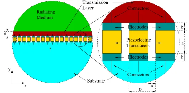
First, we compute the harmonic magnitude (dis-placement, potential...) for a network made of the same transducers as the final spatialy delineated probes (Fig. 1). The HFEA provides the harmonic quantities (dis-placements, charges, admittances and forces) against the excitation frequency and the parameter γ. The later is an excitation phase matching parameter between all the transducers of the probe. The computation results are obtained in a finite window containing a single trans-ducer. The link between all the transducers is due to a periodicity scheme in the HFEA. Knowing the harmonic quantities, we must compute the mutual ones and prop-agate them to reach the radiated characteristics of the probe. The mutual terms will be calculated from the harmonic ones picked up on the radiating surface. This surface is usually the frontier between the transmission medium and the radiating one (Fig. 1). In figure 1, we depicted a infinitely periodic network of transducers for a two dimension case. However, our discussion can be applied for a two dimension case as well as for a three dimension one.
As we mentioned above, we must know the mutual terms corresponding to the harmonic ones. All the pre-vious magnitudes could be taken into account but we
Transducers’ Piezoelectric Network Substrate y x Piezoelectric Transducers Electrodes Electrodes Transmission Layer Medium Connectors Connectors e p a h b b Radiating
Figure 1: Infinitely periodic network of acoustoelectric transducers.
have only focused on one of them.
Here, we take an interest in the displacements de-picted in figure 1.The x and (not shown) z direction are the transverse directions and y the normal direction. So, we can write the mutual displacements ua against the
harmonic ones Ua (a = {x, z} or a = y) as following:
ua(X, ν, nt) =
Z Z γXmax
γXmin
Ua(X, ν, γ) ∗ exp(2Iπntγ)dγ,
(1) where X are the coordinates vector of all the points on the base surface, ν the frequencies vector and nt the
transducers’ number in the probe[1]. In the three di-mension case, the gamma vector has one set for the x-phases and a second for the z ones. That is why there is a double integration in equation (1). In a a two dimen-sion case, It is a single integration. We also define the X vector as the γ one. It is a second rank vector in the Three dimension case, one for the x-direction and one for the z-direction.
To achieve the calculation of the normal displace-ment on the front face, we must calculate the transfer matrix for the normal displacement based on the mutual matrix uy. This transfer matrix Ty is a toeplitz table
obtained from the mutual displacement on the y-axis. This matrix is written in equation (2) page 3. where the subscripts {i, j} and k respectively denote each {x, z}-position in a transducer and each frequency. τ stands in for the two vectors X and ν. The toeplitz matrix Ty is the matrix defining all the relations between the
different transducer building up the probe. These rela-tions are normalized by the potential excitation of each transducers. So we must know the activation potentials of the whole probe to calculate the normal displacement on the front face.
Therfore, we define a vector φ which define the elec-tric potential used to excite each transducer. So, the dimension of the vector φ is nt. To simplify our
dis-cussion, we can define phi(i) = 0 when the transducer i is not activated and phi(i) = 1 when it is. Thus, we are able to determinate the front face displacement Υy(X, nt) for a specified frequency at every points of
θ φ Component Acoustic r x y z xmax zmax s s M(x ,y ,z )s
Figure 2: Configuration of the front face informations propagation.
each transducer:
Υy(X, νi, nt) = Ty(X, νi, nt, nt)φ(nt), (3)
the multiplication is on the last dimension of Ty.
Now, we propagate the known informations on the front face into the radiating medium. For instance, we afford to calculate the pressure yielded by our probe on sphere of radius r (figure 2). The pressure on the sphere P (Xs, ys, ω) is defined by the equation (4).
P (Xs, ys, ω) = Z X0=Xmax X0=−X max ρfω2 Υy(X0, ω)G(Xs− X0, ys, ω)dX0 (4)
where Xs and ys are the coordinates of the sphere
points, −Xmaxand Xmax are the limits of the acoustic
component, ρf is the density of the radiating medium,
omega = 2πν is the pulsation of the excitation and G(Xs− X0, ys, ω) is the green function related to the
radiating medium[2]. The X coordinates have the same definition as above for the three dimension case. So the integration in equation (4) is on x and z, it is a dou-ble integration. The Green function is defined by the equation (5) for the two dimension case[3].
G(xs− x0, ys, ω) =
H2 0(kr)
Ty(τi,j,k, nt, nt) =
uy(τi,j,k, 1) uy(τi,j,k, 2) uy(τi,j,k, 3) · · · uy(τi,j,k, nt− 2) uy(τi,j,k, nt− 1) uy(τi,j,k, nt)
uy(τi,j,k, 2) uy(τi,j,k, 1) uy(τi,j,k, 2) · · · uy(τi,j,k, nt− 3) uy(τi,j,k, nt− 2) uy(τi,j,k, nt− 1)
uy(τi,j,k, 3) uy(τi,j,k, 2) uy(τi,j,k, 1) · · · uy(τi,j,k, nt− 4) uy(τi,j,k, nt− 3) uy(τi,j,k, nt− 2)
..
. ... ... . .. ... ... ...
uy(τi,j,k, nt− 2) uy(τi,j,k, nt− 3) uy(τi,j,k, nt− 4) · · · uy(τi,j,k, 1) uy(τi,j,k, 2) uy(τi,j,k, 3)
uy(τi,j,k, nt− 1) uy(τi,j,k, nt− 2) uy(τi,j,k, nt− 3) · · · uy(τi,j,k, 2) uy(τi,j,k, 1) uy(τi,j,k, 2)
uy(τi,j,k, nt) uy(τi,j,k, nt− 1) uy(τi,j,k, nt− 2) · · · uy(τi,j,k, 3) uy(τi,j,k, 2) uy(τi,j,k, 1)
(2)
In equation (5), H0 is the first kind Bessel function for
the zero order, k = ω
c is the wave number and r =
p(xs− x0)2+ (ys− y0)2. For a three dimension case,
the Green function becomes G(xs− x0, ys, ω) =
1
4πrexp (−jkr) (6) with r =p(xs− x0)2+ (ys− y0)2+ (zs− z0)2.
In this work, we choose to apply this method for the directivity. However, it could be applied for all the cases named above in the introduction (the crosstalk, the output, the transfer function...).
3
Test cases and discussions
We carry out the geometric configuration from an ex-perimental set up devoted to the design of the medical probes.
Figure 3: Geometric configuration of one cell of the acoustic probe. It is a stack of different materials: backing, electrodes, PZT, quartz and adaptation layer.
We depicted in figure 3 one of the cell forming the whole probe. The probe is made by a finite network of eleven transducers defined in Fig. 3. Those transduc-ers are made by a stack of laytransduc-ers of 500 µm high and 100 µm wide. The PZT layer is activated by a potential
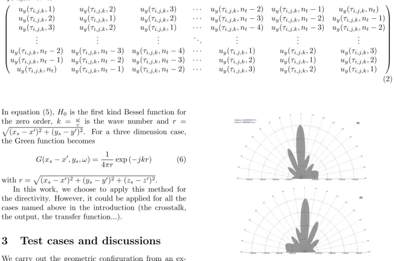
Figure 4: Pressure (Pa) generated by acoustic probe in water depicted on the Sommerfeld sphere (r=1 m). The φ-angle is set to zero. the grey graduations stand for the θ-angle. Angles are in degrees. (a) only the first
transducer is activated at 2000 kHz. (b) The same configuration for the eleventh transducer at 2000 kHz.
All the other activation potentials are null.
difference between two electrodes (Fig. 3). The wave created by the acoustic probe propagates in the radia-tion medium. This medium is water and the wave is transmitted by the polymer layer. The frequency range of excitation is between 500 and 5000 kHz. We are capa-ble to excite all the transducers or only one of them. In this paper, we only show results for this two dimension configuration but in further works we will discuss about Three dimensional ones.
First, The transducers of the probe are activated one by one. We show here the behavior of the probe when only the transducers placed at the extremities of the probe are activated, i.e. the first one and af-ter the eleventh. The frequency of excitation is set to 2000 kHz. All the potentials are null excepted the cho-sen one. The transducer number one is on the left of the probe whereas the last one is on the right. In fig-ure 4(a), we depicted the pressfig-ure emitted by the probe in water when only the first transducer is on. We can see a lobe for θ = 0 which is the zero order of prop-agation and a diffraction pattern due to the coupling between the transducers. In figure 4(b), we show the same configuration than in figure 4(a) when the eleventh transducer is activated. The two curves are symmetric
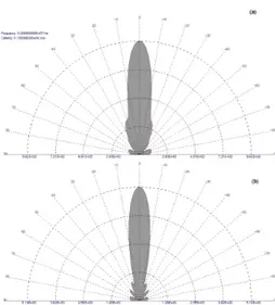
Figure 5: Pressure (Pa) generated by acoustic probe in water depicted on the Sommerfeld sphere (r=1 m). The φ-angle is set to zero. the grey graduations stand
for the θ-angle. Angles are in degrees. (a) only the sixth transducer is activated at 2000 kHz. (b) The same configuration for the forth, fifth, sixth, seventh
and eighth transducers at 2000 kHz. All the other activation potentials are null.
Figure 6: Pressure (Pa) generated by acoustic probe in water depicted on the Sommerfeld sphere (r=1 m). The φ-angle is set to zero. the grey graduations stand
for the θ-angle. Angles are in degrees. only the first transducer is activated. (a) The frequency activation is set to 1000 kHz, (b) 4000 kHz. All the other activation
potentials are null.
(f1(θ) = f11(−θ)). In fact, All the used materials
form-ing the probe have an isotropic behavior in the radiation plane (x-z). So, the global behavior does not depend on the propagation direction in the plane (x-z).
Next, we change the number of activated transduc-ers. We begin to activate the central transducer and we continue by activating its four closest neighbors. The excitation frequency is the same as previously. This re-sult is depicted in figure 5(a) for the single activated transducer and (b) for the case with five activated trans-ducers. The most significant difference between the two configurations is the intensity of the radiated pressure. This slightly change the coupling between the cells of the probe. This remark is highlighted by the differences between the secondary lobes of the two figures 5.
At last, we only activate the first transducer and we vary the excitation frequency. In figure 6(a) and (b), we respectively depicted the radiated pressure for ex-citation frequency set to 1000 kHz and 4000 kHz. We can also take into account the figure 4(a) which depicted our last configuration for a excitation frequency set to 2000 kHz. We can see on these three figure that the zero order lobe contribution decreases when the frequency in-creases. It completely vanishes for the high frequencies. Apparently, the coupling between the transducers of the probe seems to become higher when the excitation fre-quency increases. The secondary lobes becomes bigger than the zero order lobe and the directivity of the probe decreases.
4
Conclusion
In this paper, we demonstrate the analytical and numer-ical method to carry out the radiation characteristics of a spatially delineated acoustic probe from a numerical analysis of an infinitely periodic network of transducers. We also discuss the results obtained from an ex-perimental set up. We demonstrate we are capable to characterized an acoustic probe radiating in a isotropic medium. We show some two dimension results. The three dimension work will be presented in further works.
Acknowledgment
We would like to thank F. Lanteri and J.F. Gelly (GE Healthcare, Sophia Antipolis, France) for the experi-mental set up design and the fruitful discussions.
References
[1] Y. Zhang, J. Desbois et L. Boyer, ”Characteristic parameters of surface acoustic waves in a periodic metal grating on a piezoelectric substrate.” IEEE Trans. Ultrason., Ferroelect., Freq. Contr., 40(3), 183-192, (1993).
[2] L.E. Kinsler, A.R. Frey, A.B. Coppens et J.V. Senders, ”Fundamentals of Acoustics.”, chapitre 5. Wiley, 4th ˜A c dition, (2000).
[3] C. Lesueur, ”Rayonnement Acoustique des Struc-tures.”, chapitre 3. Eyrolles, (1988).