A Test for the Presence of Central Bank Intervention in the Foreign Exchange Market With an Application to the Bank of Canada

Texte intégral

(1)2009s-14. A Test for the Presence of Central Bank Intervention in the Foreign Exchange Market With an Application to the Bank of Canada Douglas James Hodgson. Série Scientifique Scientific Series. Montréal Avril 2009. © 2009 Douglas James Hodgson. Tous droits réservés. All rights reserved. Reproduction partielle permise avec citation du document source, incluant la notice ©. Short sections may be quoted without explicit permission, if full credit, including © notice, is given to the source..

(2) CIRANO Le CIRANO est un organisme sans but lucratif constitué en vertu de la Loi des compagnies du Québec. Le financement de son infrastructure et de ses activités de recherche provient des cotisations de ses organisations-membres, d’une subvention d’infrastructure du Ministère du Développement économique et régional et de la Recherche, de même que des subventions et mandats obtenus par ses équipes de recherche. CIRANO is a private non-profit organization incorporated under the Québec Companies Act. Its infrastructure and research activities are funded through fees paid by member organizations, an infrastructure grant from the Ministère du Développement économique et régional et de la Recherche, and grants and research mandates obtained by its research teams. Les partenaires du CIRANO Partenaire majeur Ministère du Développement économique, de l’Innovation et de l’Exportation Partenaires corporatifs Banque de développement du Canada Banque du Canada Banque Laurentienne du Canada Banque Nationale du Canada Banque Royale du Canada Banque Scotia Bell Canada BMO Groupe financier Caisse de dépôt et placement du Québec DMR Fédération des caisses Desjardins du Québec Gaz de France Gaz Métro Hydro-Québec Industrie Canada Investissements PSP Ministère des Finances du Québec Power Corporation du Canada Raymond Chabot Grant Thornton Rio Tinto Alcan State Street Global Advisors Transat A.T. Ville de Montréal Partenaires universitaires École Polytechnique de Montréal HEC Montréal McGill University Université Concordia Université de Montréal Université de Sherbrooke Université du Québec Université du Québec à Montréal Université Laval Le CIRANO collabore avec de nombreux centres et chaires de recherche universitaires dont on peut consulter la liste sur son site web. Les cahiers de la série scientifique (CS) visent à rendre accessibles des résultats de recherche effectuée au CIRANO afin de susciter échanges et commentaires. Ces cahiers sont écrits dans le style des publications scientifiques. Les idées et les opinions émises sont sous l’unique responsabilité des auteurs et ne représentent pas nécessairement les positions du CIRANO ou de ses partenaires. This paper presents research carried out at CIRANO and aims at encouraging discussion and comment. The observations and viewpoints expressed are the sole responsibility of the authors. They do not necessarily represent positions of CIRANO or its partners.. ISSN 1198-8177. Partenaire financier.

(3) A Test for the Presence of Central Bank Intervention in the Foreign Exchange Market With an Application to the Bank of Canada Douglas James Hodgson *. Résumé / Abstract Nous proposons un cadre de référence général pour les équations non-linéaires simultanées s’appliquant à l’analyse économétrique de modèles d’intervention des banques centrales dans les marchés des devises étrangères, en réponse aux écarts des taux de change par rapport aux niveaux cibles. Nous prenons en considération l’estimation des variables instrumentales liées aux fonctions de réponses possiblement non-linéaires et aux tests en matière d’interventions lorsque la forme fonctionnelle peut être non linéaire, asymétrique et lorsqu’elle peut contenir des paramètres de forme inconnue. La méthodologie applique, à un modèle à équations simultanées non linéaires, des techniques élaborées pour effectuer des tests en présence de paramètres de nuisance non identifiés sous une hypothèse nulle. Nous présentons les résultats d’une analyse empirique des activités de la Banque du Canada, durant la période de 1953-2006, relativement au taux de change Canada-É.-U., les variations des réserves étrangères permettant les activités d’intervention.. Mots clés : paramètre de nuisance non identifié, équations simultanées non linéaires, réserves de change, fonctions de réaction de la politique.. We propose a general non-linear simultaneous equations framework for the econometric analysis of models of intervention in foreign exchange markets by central banks in response to deviations of exchange rates from target levels. We consider the instrumental variables estimation of possibly non-linear response functions and tests of intervention when the functional form may be non-linear, asymmetric, and may contain unknown shape parameters. The methodology applies techniques developed for testing in the presence of nuisance parameters unidentified under a null hypothesis to a nonlinear simultaneous equations model. We report the results of an empirical analysis of activity of the Bank of Canada, for the period from 1953-2006, with regard to the Canada-U.S. exchange rate, with changes in foreign reserves proxying for intervention activity. Keywords: unidentified nuisance parameter, nonlinear simultaneous equations, foreign exchange reserves, policy reaction functions.. *. Université du Québec à Montréal and CIRANO, Douglas.Hodgson@cirano.qc.ca.

(4) A TEST FOR THE PRESENCE OF CENTRAL BANK INTERVENTION IN THE FOREIGN EXCHANGE MARKET WITH AN APPLICATION TO THE BANK OF CANADA. 1. INTRODUCTION There exists a substantial empirical literature seeking to estimate the function characterizing the policy response of a central bank to deviations of an exchange rate from a target level (for surveys, see Almekinders and Eijffinger (1991) and Sarno and Taylor (2001)), but little work has been dedicated to the specific question of testing for the presence or absence of such a policy response. If policy-makers are assumed to have a reaction function that is linear in the exchange rate deviation, then there is no problem here, as testing for the absence of policy reaction reduces to testing a point hypothesis on the value of a parameter in a linear regression model, and thus to the question of estimation of this parameter. If the reaction function is allowed to contain nonlinearity - and there are good reasons why an empirical investigator may wish to allow this - then the testing issue.

(5) becomes more complicated. The monetary authority responds to deviations of an exchange rate from its target level through variations in a policy variable which are intended to counter these deviations. There is not unanimity in the literature regarding the appropriate functional form of the policy response function, and, due to a lack of economic theory specifying its form, this function is often specified on an ad hoc basis in empirical work (but see Almekinders and Eijffinger (1996) for an exception). Although linear specifications are often employed in practice, various sources of nonlinearity are plausible, such as, for example, asymmetry (if a central bank places greater weight on depreciations than on appreciations), convexity of the reaction function (the reaction becomes increasingly strong the greater is the deviation of the exchange rate from its target), and threshold effects (intervention doesn’t occur unless the deviation from target is sufficiently large), or combinations of the above. This possibility of nonlinearity poses important econometric complications. Even if the functional specification has theoretical support, there may be parameters present in the function whose value is not specified in advance and must be estimated. A similar problem arises even when the specification of the functional form is essentially ad hoc, a situation where we would also be interested in applying a test of functional form. Whatever the case, the essential non-linearity of the model implies that any such test will have non-standard properties, belonging to the category of tests for which there exist nuisance parameters that are unidentified under the null hypothesis. Econometric methods are now available to handle such situations (for example, Andrews and Ploberger (1994) and Hansen (1996)), and their applicability to the problem at hand will be investigated in this paper. We should add that a second source of econometric complication must also be addressed in testing for the presence of a particular policy reaction function, namely, the issue of simultaneity. It is reasonable to expect that changes in a correctly-chosen policy variable will rapidly feed back into movements of the exchange rate itself. Hence, it would be desirable to specify a non-linear simultaneous equations model in which a second equation characterizing this feedback effect is included The contribution of this paper is to develop and apply an econometric test for the existence of central bank intervention which uses the results of Andrews and Ploberger (1994) and Hansen (1996) to allow for the specification of a nonlinear parametric intervention function and the presence of endogeneity in the model. Despite the fact that endogeity and nonlinearity have both been addressed in the literature at various times and by various authors (see the surveys of Almekinders and Eijffinger (1991) and Sarno and Taylor (2001)), the two phenomena have rarely been combined in a single econometric framework, and no actual testing has been undertaken regarding the validity of the specification of a particular nonlinear functional form. In particular, no test that addresses the problem of possibly unidentified nuisance parameters appears to have been applied in the literature, even though it seems to us that such an approach is the correct way to address the testing problem. Our model is presented in Section 2, the test described in Section 3, and Section 4 reports the results of an application to activity of the Bank of Canada during the period 1953-2006.. 2. THE MODEL.

(6) Suppose that, for each period t  1, . . . , n, we observe an exchange rate (generally expressed in logs), s t , and some policy instrument, i t . There is a target exchange rate, s ∗t , and policy reacts to deviations from target according to the following relationship: i t  gd t , , 1 ∗ where d t  s t − s t , g is a specified nonlinear function with unknown parameter vector , and the slope parameter  will equal zero if there is no policy reaction or if the functional form of g is incorrectly specified. The null hypothesis   0 will thus be of central interest for us. Note that the parameter vector  is unidentified under the null, which will create problems in its testing. We introduce a sequence of  −fields F t , and assume that the pair s t , i t  is measurable with respect to F t . In addition, suppose that a vector z t , measurable with respect to F t−1 , of auxiliary variables is observed, which may contains lags of s t , i t , in addition to other economic variables that may be relevant to our model. Suppose that the target rate is a known function of z t , s ∗t  hz t , say, and that the bivariate sequencey t   d t , i t  is stationary and ergodic. The first equation in our econometric model is derived from (1) by writing 2 i t   0   1 gd t ,   q 1 z 1t ,  1   u 1t , where q 1 z 1t ,  1  is a known function, z 1t is the sub-vector of z t containing those elements that are not excluded from q 1 z 1t ,  1  on a priori grounds,  1 is an unknown parameter vector with p 1 elements, to be estimated, and u 1t  is an iid sequence of disturbances with density f 1 u 1 . We assume that u 1t is independent of z t , but not necessarily of d t . The possible endogeneity of the regressor d t arises from the fact that simultaneity can be present in our system if the instrument i t feeds back into the equation determining the exchange rate s t (we would expect such feedback to exist if i t is an effective instrument). The inclusion of the term q 1 z 1t ,  1  reflects the presence of factors other than the current exchange rate deviation that may influence the behavior of i t . We would expect, for example, that lags of i t would enter z 1t if this variable exhibits any degree of persistence. Those elements of z t that are excluded from q 1 z 1t ,  1  furnish possible instruments in the instrumental variables estimation of . To fix ideas, consider a model in which i t is the policy instrument of the central bank of a small open economy, and s t is the domestic-currency price of a unit of the currency of a larger foreign economy, so that a positive value of d t indicates that the domestic currency is undervalued relative to the central bank’s target rate s ∗t . For example, if i t were the change in reserve holdings of the foreign currency by the domestic central bank (a positive value of which would then be expected to have a depressing effect on the value of the domestic currency), and if gd t ,  were an increasing function of d t , then one would expect  1 to be less than zero. Although there may be little theoretical basis to prefer one specification of the functional form of gd t ,  to another (but see Almekinders and Eijffinger (1996)), the following specification has some desirable properties, as described below:  gd t ,   d t Id t  0 − |d t |  Id t  0, 3 where I denotes the indicator function. In this example, the parameter vector of gd t ,  is   , . The members of  have economically interesting interpretations. The shape of the reponse function will be governed by , with a value of unity indicating linear policy response and progressively larger values representing a convex policy response, i.e. one that is less responsive to small deviations from target and more responsive to larger.

(7) deviations. We would not generally expect  to be less than one.  is expected to be positive, with a value of unity reflecting policy which responds equally strongly to a relatively devalued and relatively overvalued currency. There may be reason to expect the central bank to be more sensitive to devaluations of the currency, in which case we would have 0    1. The simultaneous equations system is completed with the following equation characterizing the feedback of the instrument into the exchange rate: 4 d t   2   3 i t  q 2 z 2t ,  2   u 2t , where q 2 z t ,  2  is a known function, z 2t contains the elements of z t that are not excluded from q 2 z 2t ,  2 ,  2 is an unknown parameter vector with p 2 elements, to be estimated, and u 2t  is an iid sequence of disturbances with density f 2 u 2 . Note that z 1t and z 2t are not prohibited by definition from having common elements. We assume here that the feedback of the instrument into the exchange rate is linear, an assumption that can easily be relaxed. The term q 2 z 2t ,  2  will often contain lags of d t . We assume that u 2t is independent of z t , but not necessarily of i t . The bivariate sequence u t  u 1t , u 2t  T is iid from the density fu. The superscript T denotes transposition of a vector or matrix. As mentioned, the terms q 1 z 1t ,  1  and q 2 z 2t ,  2  are included to capture time series dynamics that may be present in the series i t  and d t , respectively. One possible approach to the specification of these terms would be as autoregressions in the dependent variable of the respective equations, so that we would have p1. q 1 z 1t ,  1  . ∑  1j i t−j   T1 z 1t. 5. j1. and p2. q 2 z 2t ,  2  . ∑  2j d t−j   T2 z 2t , j1. where z 1t  i t−1 , . . . , i t−p 1  and z 2t  d t−1 , . . . , d t−p 2 . We would then have the lags of the excluded variables available as instruments for the consistent estimation of (2) and (4). For example, lagged values of i t could be used as instruments for the estimation of  3 in (4), and nonlinear functions of lagged values of d t could be used as instruments for the IV estimation of  1 and  in (2). We shall assume for now that valid instruments are available, so that equations (2) and (4) are identified. We note here that a question that may need to be addressed in practice, particularly with respect to estimation of (2), is the quality of the instruments employed.. 3. TESTING FOR THE PRESENCE AND SPECIFICATION OF THE POLICY REACTION FUNCTION As mentioned above, we are interested, for various reasons, in the question of testing the null hypothesis of  1  0 in (2). This is an unusual and interesting problem because the parameter  is unidentified under the null hypothesis but not under the alternative, creating a nonstandard testing problem which several authors have considered. Andrews and. 6.

(8) Ploberger (1994) obtain a class of optimal tests, but don’t say much about implementation or computation of critical values (the tests have nonstandard distributions). The issue of critical values is addressed by Hansen (1996), who provides an illustration through an empirical example. To apply the general methods of Andrews and Ploberger (1994) and Hansen (1996) to the problem of testing the null hypothesis of  1  0 in (2), one must begin by estimating the parameters  0 ,  1 , and  1 in equation (2), holding  fixed, for each point  in the parameter space B. Since, for given , the equation regression becomes linear, with regressor vector T v 1t   1, g t , z T1t  , where g t   gd t , , the equation can be estimated by ordinary least squares (OLS), or, if g t  is endogenous, by instrumental variables (IV), where some instrument g ∗t  1 is used, yielding the instrument vector T v ∗1t   1, g ∗t , z T1t  . For given , denote by  1n  our estimator of  1 . The tests of Andrews and Ploberger (1994) involve computing LM, LR, or Wald statistics of the null for various values of , and then computing a weighted average (over the set of possible values of ) of these statistics. For each choice of , we can compute a Wald, LM, or LR statistic of the null hypothesis that  1  0. The Wald test, for example, would be n  21n  W n   . 7 se  1n  The denominator in (7) is a consistent estimator of the asymptotic standard deviation of the estimator. The exponential Wald test as suggested by Andrews and Ploberger then takes the form Exp − W n  1  c −1/2  exp. c W n  dJ, 8 21  c where c and J are user-defined constant and weight function, respectively, whose choice is discussed by Andrews and Ploberger (1994). The limit of the statistic in (8) as c → 0 is the "average-Wald" ("ave-W") statistic B. B W n dJ,. while its limit as c →  is. B exp. 1 W n  dJ, 2 and will be referred to below as "log-exp-W". The resulting statistic will have a nonstandard limiting distribution, computation of the p-values of which is considered by Hansen (1996). Note that in practice it may be necessary to compute W n  for a discrete set of points  belonging to the parameter space. A method of conducting inference with the statistic given in (8) which follows the lines of Hansen (1996), is outlined in the Appendix. log. 4. INTERVENTION BY THE BANK OF CANADA. 9. 10.

(9) Canada is a classic example of a small open economy, the lion’s share of whose foreign trade is with its mammoth neighbour, the United States. The exchange rate between the Canadian and U.S dollars is thus of great interest and importance to Canada, and it is plausible that the rate is closely monitored, and possibly influenced, by the Bank of Canada. A number of attempts have been made to econometrically measure the nature and extent of the Bank of Canada’s intervention in the foreign exchange market (for example, Longworth (1980), Weymark (1995), and Rogers and Siklos (2003)). According to the following quotation, taken from the Bank’s website 2 and dated July 2001, it has in recent years refrained from such intervention: The Bank of Canada influences the exchange rate only indirectly. This can happen when the Bank changes its Target for the Overnight Rate, which affects short-term interest rates. As of 1998, the Bank no longer intervenes in foreign exchange markets to ensure an orderly market, but rather reserves such actions for times of major international crisis or a clear loss of confidence in the currency or Canadian-dollar-denominated securities. The test outlined in the preceding section, applied to Canadian data for the period 1953-2006 (with certain subperiods being considered separately), would thus constitute a test of the null hypothesis that the Bank’s public utterance of a no-intervention policy is an accurate reflection of its true behaviour. We proceed with such an analysis in this section. Before presenting our results, we discuss various details relating to the application of the methodology.. 4.1 Data and Measurement of Variables The first step in any study of foreign exchange market intervention is to define precisely what will be meant by “intervention”. How is it measured in practice, using available data series? Secondly, in estimating the response of the intervention variable to deviations of the exchange rate from its target, we must somehow measure or estimate a (generally time-varying) target exchange rate. Various approaches have been taken to the definition of both of these variables, as can be seen by a quick perusal of the literature survey of Almekinders and Eijffinger (1991). 3 Many authors use changes in foreign reserve holdings, possibly modified to account for changes in reserves due to factors other than intervention, as a measure of intervention. For studies in the Canadian context, see, for example, Dornbusch (1980), Longworth (1980), Weymark (1995), and Rogers and Siklos (2003). We use as our measure of intervention the log first difference in the Bank of Canada’s official international reserves of U.S. dollars. One must also specify the target exchange rate s ∗t . In the absence of an explicitly stated target rate, the specification here is largely left to the discretion of the researcher. The target is often taken to be the previous period’s exchange rate, so that intervention is modelled as being a reaction to any change in the exchange rate, which is essentially the approach taken in this paper. We apply our test for two data sets. The first consists of monthly observations of the.

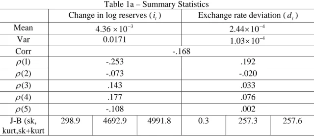
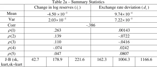
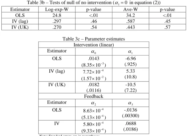
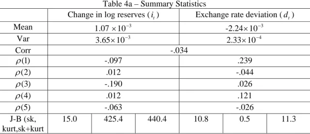
(10) Canada-U.S. exchange rate and the Bank of Canada’s official foreign reserves of U.S. dollars, obtained from Statistics Canada, for the period January, 1953 to November, 2006 (the series are plotted in Figures 2 and 3). In this case, the target exchange rate is just taken to be the first lag. As the Canadian dollar was pegged during the period June, 1962 to May, 1970, and given the above quotation from the Bank’s website, we apply our test for the entire sample period, and separately for the subperiods 1953-1962, 1970-1997, and 1998-2006. Our second data set consists of weekly observations on the same variables, from July, 1999 to November, 2006 (and plotted in Figures 4 and 5). For these data, the target rate was set as the average of the last four weeks’ realizations of the spot rate.. 4.2 Estimation and Testing - Details Tables 1-5 report our results for each of the five data sets decribed above - respectively, the monthly data for the full period and three subperiods, and the weekly data. In each case, summary statistics are provided, followed by the results of the application of the statistics given in (9) and (10) for the test of the null hypothesis that  1  0 in equation (2), with the function g specified as in (3). In applying the tests, for each value of , (2) is estimated by OLS and IV, with gd t−1 ,  being used as the instrument for gd t , . In addition, for the monthly data, a similar instrument is also used where the contemporaneous first difference of the log of the exchange rate between the British pound and the U.S. dollar replaces d t−1 . We try this additional instrument because the lack of autocorrelation in exchange rates may make d t−1 a bad instrument for d t , whereas the exchange rate between a third-country currency and the U.S. dollar should be correlated with the Canada-U.S. exchange rate while being unaffected by changes in the Bank of Canada’s U.S. dollar reserves (see Gartner (1987)). For the tests, 2500 possible values of the bivariate vector  are considered, with  values taken from the range 1-4, divided into a grid of 50 points, with the range of considered  values being .75-1, with a grid of 50 points. The weights J decline linearly in  from 1 to 4, and decline linearly in  from 1 to .75, so that maximal weight is placed on ,   1, 1, and weight zero placed on ,   4, . 75. The number of simulation draws used in the computation of the p-values is K  1000. Finally, we report the intercept and slope parameter estimates obtained in applying OLS and IV (with lagged i as the instrument) to (4), as well as to a linear version of (2), with the instruments as described above, where  and  are both restricted to equal one. Panel (a) of each Table presents some summary statistics on the data series employed. In most cases, the exchange rate and reserves series have a weak or moderate negative correlation, the exception being the weekly data, where the correlation is very weakly positive.The degree of autocorrelation in most of the series is fairly weak, particularly in the exchange rate differences. There is a moderate level of autocorrelation in the reserve changes for most of the monthly periods The Jarque-Bera (1980) statistic is generally quite small in the exchange rates (the period 1952-62 being an exception), whereas the reserve changes are highly leptokurtic. This characteristic is evident from a glance at Figures 2 and 4, where the presence of large outliers, both positive and negative, stands out. It does not seem, from eyeballing these graphs together with Figures 3 and 5, that these outliers are generally associated with substantial contrary movements in the exchange rate. Furthermore, one can observe several large swings in the exchange rate that are not accompanied by large reserve movements..

(11) The results of the application of the log-exp-W and ave-W statistics are reported in Panel (b) of each of the Tables. If we first consider Tables 4b and 5b, which report results for the post-1998 period for different data frequencies, the test does not reject the null of no intervention, at either frequency, regardless of whether the model is estimated by OLS or IV. These unanimous results are consistent with the findings in the first section of Tables 4c and 5c, where the restriction to a linear intervention function also yields no evidence of intervention. The estimation of the feedback equation in both cases yields no evidence of feedback effects, also regardless of the estimator employed. In summary, the evidence in Tables 4 and 5 is entirely consistent with the Bank’s official position that it did not intervene during this period. The evidence for earlier periods, as reported in Tables 1-3, is less clear. In all three cases, the log-exp-W and ave-W tests both strongly reject the null of no intervention when the regression (2) is estimated by OLS for fixed values of , whereas neither rejects when the regression is estimated by IV, for either of the instruments considered. In the absence of a test for exogeneity of the regressor, or of a fashion to evaluate the strength of the instruments, in models where a "matrix" of many regressions (2500, in this case) is being estimated, we cannot say which of these results is correct. The OLS result may be spurious due the the presence of endogeneity, and the IV results may be a result of the use of instruments so weakly correlated with the regressors as to render the resulting estimators too inefficient to produce powerful tests. These considerations also apply to the results obtained in restricting the reaction function to be linear (the first sections of Tables 1c, 2c, and 3c), where OLS yields a significant slope coefficient (with the predicted negative sign), whereas the IV estimates are too imprecise to yield rejections (note here that the use of a third-country exchange rate as an instrument does produce a more efficient IV estimator, markedly so for the 1953-62 period). Although the uniform rightness of the sign in the OLS estimates of the linear intervention function may lend some support to the hypothesis that endogeneity is not a problem here, one should be cautious in positing such a conclusion, particularly when one regards the estimates for the feedback equation in the final section of Tables 1c, 2c, and 3c, where OLS always yields an unexpected negative slope coefficient, with the sign being rectified by the IV estimate in two of the three cases, where a significantly positive slope estimate is produced, in conformity with the reasoning that an increase in foreign reserves would lead to a depreciation of the domestic currency.. 5. CONCLUSIONS An approach for testing for the presence of monetary authority intervention in foreign exchange markets has been proposed which incorporates the possible nonlinearity of the intervention function, as well as the possible endogeneity of the exchange rate, while applying the methodology developed by Andrews and Ploberger (1994) and Hansen (1996) for testing in the presence of a nuisance parameter that may be unidentified under the null hypothesis. The methodology is applied to samples of monthly and weekly observations on the Canada-U.S. exchange rates and the Bank of Canada’s U.S. dollar reserves, for the periods 1953-2006 and 1999-2006, respectively. Our test results strongly suggest that no intervention occurred after 1998, but are inconclusive regarding earlier periods..

(12) From an econometric standpoint, a number of possible extensions of the analysis are suggested. In particular, it would be of interest to extend the concept of a "weak instrument" to a model like ours, where an entire "matrix" of regressions is being estimated by IV, for the purpose of computing a single test statistic which integrates over all of the regressions. The weak instrument concept would need to be redefined in this context, and its implications for the behavior of the test statistic analyzed. Similarly, the development of a test for exogeneity, along the lines of a Hausman (1978) test, would also be of interest in this context. Furthermore, no attempt has been made here to model the conditional heteroskedasticity that may be present in the exchange rate. This may be important, as the central bank may want to target the volatility of the exchange rate (Almekinders and Eijffinger (1996), Rogers and Siklos (2003)). Finally, we specify the possible nonlinearity in the intervention function in a fully parametric fashion. To the extent that nonlinear intervention may be present in some other form, our test would fail to detect it, even in the absence of endogeneity and weak instrument problems. Thus, it would be of interest, in principle, to investigate the possibility of testing in the presence more general specifications. A number of possibilities exist here, from a more heavily parameterized model to a fully nonparametric one, with intermediate specifications also possible. Assuming, again, that the endogeneity and instrument relevance problems have been adequately addressed, one could estimate the functional dependence of the reserves on the exchange rates using nonparametric kernel methods (see, for example, Pagan and Ullah (1999)), with which one could test the null that the true function is horizontal. An intermediate approach suggested by Hamilton (2001) begins with a "pilot" specification that is a parametric polynomial function of the independent variable (linear in his case), to which is added an unknown function which is the result of a single random draw from a functional space according to a known and parameterized distribution function. The problem then reduces to the estimation of the parameters through the maximization of a fully specfied likelihood function, and the null of no intervention could then be expressed as a set of zero restrictions on the values of certain parameters. One advantage that our approach has over the fully nonparametric or Hamilton (2001) ones is that it incorporates certain intuitive maintained hypotheses about the nature of an intervention function - in particular, that it should be increasing and convex. It would be desirable, if working within a more flexible framework, to somehow maintain these characteristics. A final methodological point concerns the pronounced nonnormality, especially the excess kurtosis, in our intervention variable. Given that we have made reference in analyzing our results to the problems of efficiency of estimation, the presence of thick tails in our data imply significant efficiency losses for the least squares style estimators employed throughout our analysis. Potentially substantial efficiency gains could be possible through the specification of a non-Gaussian parametric density, or the semiparametric efficient estimation of the model, in treating the functional form of the likelihood function nonparametrically (Brown and Hodgson (2007)).. 6. APPENDIX - CALCULATION OF P-VALUES.

(13) To illustrate the idea behind the procedure suggested by Hansen (1996) 4 , we consider the application of the procedure to the IV estimator, for any given value of , of the T parameter vector  1   0 ,  1 ,  T1  , where the instrument vector is v ∗1t  The null hypothesis that  1  0 can be expressed as the null that R T  1  0, where R is a vector of dimension 2  p 1 whose elements are all zeros, excepting the second, which is a one. The “regression score” defining  1n  is s t   v ∗1t u 1t and its estimated version is   s t   v ∗1t  u 1t ,  where u 1t is the residual from the IV estimator  1n . Now define the following matrices: n. M n,ss   n. −1. ∑ s t s t  T , t1. and n. M n,v∗v  1 ,  2   n. −1. ∑ v ∗1t  1 v 1t  2  T , t1. where  1 and  2 are possibly different points in the parameter space B. The asymptotic covariance matrix of  1n  is then consistently estimated by −1   1   M n,v∗v , M n,ss M n,v∗v ,  −1T . The Wald statistic W n  defined in (7) can then be rewritten as follows:. W n   n  1n  T R R T   1 R. −1. R T  1n .. Now, suppose that we have used a random number generator to supply a sequence of iid standard normal random variables  t  nt1 . Define the statistics n  −1/2 S n   n ∑ s t  t. A.1. t1. and  −1 W n   S n  T M n,v∗v , R R T   1 R. −1.  R T M n,v∗v ,  −1T S n .. To compute the p-value of our Exp − W n statistic given in (8), we generate K different sequences of iid random normals,  k  nt1 , k  1, . . . , K, and for each k, we use the k k definitions (A.1) and (A.2) to compute S n and W n , the latter of which can be substituted into (8) to give us the statistic Exp − W kn  1  c −1/2  exp. k. c W  dJ. 21  c n B The asymptotic p-value of the Exp − W n statistic computed from the data will then be estimated to an arbitrarily high degree of accuracy by the proportion of the simulated Exp − W kn statistics that exceed it.. A.2.

(14) NOTES 1. For now, we ignore the important issues of instrument relevance and multiple instruments. Suppose that g ∗t  is optimal among what may be a larger number of available instruments, i.e. that it is the instrument we would use in computing two stage least squares. 2. http://www.bankofcanada.ca/en/backgrounders/bg-e1.htm 3. A more recent survey of work in this area is provided by Sarno and Taylor (2001). 4. We should note that Hansen’s (1996) theory applies only to OLS estimation of linear models with exogenous regressors. We are unaware of the existence of theoretical results extending this analysis to estimation by linear IV methods such as 2SLS. ACKNOWLEDGEMENTS. REFERENCES Almekinders, G.J. and Eijffinger, S. 1991. Empirical evidence on foreign exchange market intervention: Where do we stand? Weltwirtschafliches Archiv 127:645-677. Almekinders, G.J. and Eijffinger, S. 1996. A friction model of daily Bundesbank and Federal Reserve intervention. Journal of Banking and Finance 20:1365-1380. Andrews, Donald W.K. and Ploberger, Werner. 1994. Optimal tests when a nuisance parameter is present only under the alternative. Econometrica 62:1383-1414. Brown, B.W. and Hodgson, D.J. 2007. Semiparametric efficiency bounds in dynamic nonlinear systems under elliptical symmetry. Forthcoming, Econometrics Journal. Dornbusch, R. 1980. Exchange rate economics: Where do we stand? Brookings Papers on Economic Activity 1:143-185. Gartner, M. 1987. Intervention policyunder floating exchange rates: An analysis of the Swiss case. Economica, New Series 54:439-453. Hamilton, J.D. 2001. A parametric approach to flexible nonlinear inference. Econometrica 69:537-573. Hansen, Bruce E. 1996. Inference when a nuisance parameter is not identified under the null hypothesis. Econometrica 64:413-430. Hausman, J. 1978. Specification tests in econometrics. Econometrica 46:1251-1271..

(15) Longworth, D. 1980. Canadian intervention in the foreign exchange market: A note. Review of Economics and Statistics 62:284-287. Newey, W.K. 1989. Locally efficient, residual-based estimation of nonlinear simultaneous equations. Bellcore Economics Discussion Paper #59. Newey, W.K. 1990. Semiparametric efficiency bounds. Journal of Applied Econometrics 5:99-135. Pagan, A. and Ullah, A. 1999. Nonparametric Econometrics. Cambridge; Cambridge Univ. Press. Rogers, J.M. and Siklos, P.L. 2003. Foreign exchange market intervention in two small open economies: The Canadian and Australian experience. Journal of International Money and Finance 22:393-416. Sarno, Lucio and Taylor, Mark P. 2001. Official intervention in the foreign exchange market: Is it effective and, if so, how does it work? Journal of Economic Literature 39:839-868..

(16) Table 1 – Monthly Data, 1953-2006 Table 1a – Summary Statistics Change in log reserves ( it ) Exchange rate deviation ( d t ) Mean 4.36 × 10 −3 2.44 × 10 −4 Var 0.0171 1.03 × 10−4 Corr -.168 ρ (1) -.253 .192 ρ (2) -.073 -.020 ρ (3) .143 .033 ρ (4) .177 .076 -.108 .002 ρ (5) J-B (sk, 298.9 4692.9 4991.8 0.3 257.3 257.6 kurt,sk+kurt Note: ρ ( j ) indicates the autocorrelation at lag j, and J-B refers to the Jarque-Bera (1980) skewness, kurtosis, and skewness-kurtosis statistics. Table 1b – Tests of null of no intervention ( α1 = 0 in equation (2)) Estimator Log-exp-W p-value Ave-W p-value OLS 20.07 <.01 21.04 <.01 IV (lag) .97 .16 1.81 .16 IV (UK) .31 .52 .50 .56. Table 1c – Parameter estimates Intervention (linear) Estimator α0 α1 OLS -3.33 6.61 × 10 −3 −3 (.495) (4.83 × 10 ) 5.60 IV (lag) 3.69 × 10 −3 −3 (3.94) (6.05 × 10 ) -4.79 IV (UK) 7.09 × 10 −3 −3 (3.21) (4.97 × 10 ) Feedback Estimator α2 α3 − 4 -.0147 OLS 2.49 × 10 −4 (.00295) (3.85 × 10 ) − 4 .0812 IV -1.44 × 10 −4 (.0200) (6.29 × 10 ) Note: Standard errors are in parentheses.

(17) Table 2 – Monthly Data, 1953-1962. Table 2a – Summary Statistics Change in log reserves ( it ) Exchange rate deviation ( d t ) Mean 9.74 × 10 −4 -4.50 × 10 −3 Var 7.22 × 10 −5 2.03 × 10 −3 Corr -.386 ρ (1) .263 .00143 ρ (2) .139 -.0722 ρ (3) .110 -.0416 ρ (4) -.074 .0242 .047 .0807 ρ (5) J-B (sk, 42.7 178.9 221.6 162.3 1004.3 1166.6 kurt,sk+kurt Note: ρ ( j ) indicates the autocorrelation at lag j, and J-B refers to the Jarque-Bera (1980) skewness, kurtosis, and skewness-kurtosis statistics. Table 2b – Tests of null of no intervention ( α1 = 0 in equation (2)) Estimator Log-exp-W p-value Ave-W p-value OLS 5.07 <.01 8.08 <.01 IV (lag) 1.28 .12 2.38 .13 IV (UK) 1.06 .17 2.10 .17 Table 2c – Parameter estimates Intervention (linear) Estimator α0 α1 OLS -1.79 -1.94 × 10 −3 −3 (.447) (3.92 × 10 ) -10.95 IV (lag) 4.62 × 10 −3 −2 (8.94) (1.03 × 10 ) -1.05 IV (UK) -2.47 × 10 −3 −3 (.766) (3.99 × 10 ) Feedback Estimator α2 α3 − 4 -.0735 OLS 5.75 × 10 −4 (.0166) (7.52 × 10 ) − 4 -.174 IV 1.03 × 10 −4 (.0585) (9.06 × 10 ) Note: Standard errors are in parentheses.

(18) Table 3 – Monthly Data, 1970-1997. Table 3a – Summary Statistics Change in log reserves ( it ) Exchange rate deviation ( d t ) Mean 5.04 × 10 −3 9.63 × 10 −4 Var .0291 9.41 × 10 −5 Corr -.220 ρ (1) -.308 .180 ρ (2) -.089 -.020 ρ (3) .168 .033 ρ (4) -.190 .039 ρ (5) .144 -.045 J-B (sk, 91.1 696.6 787.7 16.6 1.0 17.6 kurt,sk+kurt Note: ρ ( j ) indicates the autocorrelation at lag j, and J-B refers to the Jarque-Bera (1980) skewness, kurtosis, and skewness-kurtosis statistics. Table 3b – Tests of null of no intervention ( α1 = 0 in equation (2)) Estimator Log-exp-W p-value Ave-W p-value OLS 24.8 <.01 34.2 <.01 IV (lag) .297 .46 .587 .45 IV (UK) .270 .54 .443 .57 Table 3c – Parameter estimates Intervention (linear) Estimator α0 α1 OLS .0143 -6.96 −3 (.925) (8.35 × 10 ) − 4 IV (lag) 5.33 7.72 × 10 −2 (10.8) (1.57 × 10 ) IV (UK) .0182 -10.5 (.0116) (7.22) Feedback Estimator α2 α3 OLS IV. 8.63 × 10 −4 (5.13 × 10−4 ) 5.80 × 10 −4 (9.33 × 10−4 ). Note: Standard errors are in parentheses. -.0136 (.00300) .0688 (.0186).

(19) Table 4 – Monthly Data, 1998-2006 Table 4a – Summary Statistics Exchange rate deviation ( d t ) Change in log reserves ( it ) Mean 1.07 × 10 −3 -2.24 × 10 −3 Var 3.65 × 10 −3 2.33 × 10 −4 Corr -.034 ρ (1) -.097 .239 ρ (2) .012 -.044 ρ (3) -.190 .026 ρ (4) .012 .121 -.063 -.026 ρ (5) J-B (sk, 15.0 425.4 440.4 10.8 0.5 11.3 kurt,sk+kurt Note: ρ ( j ) indicates the autocorrelation at lag j, and J-B refers to the Jarque-Bera (1980) skewness, kurtosis, and skewness-kurtosis statistics. Table 4b – Tests of null of no intervention ( α1 = 0 in equation (2)) Estimator Log-exp-W p-value Ave-W p-value OLS .067 .73 .130 .73 IV (lag) .722 .26 1.42 .23 IV (UK) .339 .44 .669 .43 Table 4c – Parameter estimates Intervention (linear) Estimator α0 α1 OLS -.136 -1.05 × 10 −3 −3 (.363) (5.63 × 10 ) 2.06 (1.79). IV (UK). 3.79 × 10 −3 (7.58 × 10 −2 ) 1.56 × 10 −3 (6.34 × 10 −3 ) Feedback. Estimator. α2. α3. IV (lag). OLS IV. −3. -1.66 × 10 (1.47 × 10 −3 ) -1.71 × 10 −3 (1.71 × 10 −3 ). Note: Standard errors are in parentheses. 1.05 (1.11). -.0168 (.0255) .140 (.304).

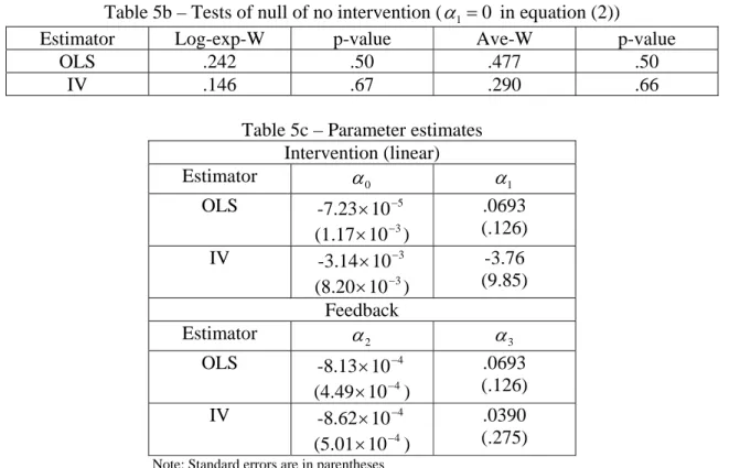
(20) Table 5 – Weekly Data, 1999-2006 Table 5a – Summary Statistics Exchange rate deviation ( d t ) Change in log reserves ( it ) Mean -1.91 × 10 −4 -7.66 × 10 −4 Var 4.77 × 10 −4 8.69 × 10 −5 Corr .026 ρ (1) .005 -.045 ρ (2) -.087 .007 ρ (3) .010 .005 ρ (4) -.037 -.004 -.072 .063 ρ (5) J-B (sk, 203.2 8451.9 8655.1 2.3 0.6 2.9 kurt,sk+kurt Note: ρ ( j ) indicates the autocorrelation at lag j, and J-B refers to the Jarque-Bera (1980) skewness, kurtosis, and skewness-kurtosis statistics. Table 5b – Tests of null of no intervention ( α1 = 0 in equation (2)) Estimator Log-exp-W p-value Ave-W p-value OLS .242 .50 .477 .50 IV .146 .67 .290 .66 Table 5c – Parameter estimates Intervention (linear) Estimator α1 α0 − 5 OLS .0693 -7.23 × 10 −3 (.126) (1.17 × 10 ) -3.76 IV -3.14 × 10 −3 −3 (9.85) (8.20 × 10 ) Feedback Estimator α2 α3 OLS IV. -8.13 × 10 −4 (4.49 × 10 −4 ) -8.62 × 10 −4 (5.01 × 10 −4 ). Note: Standard errors are in parentheses. .0693 (.126) .0390 (.275).

(21)

(22)

(23)

(24)

(25)

(26)