A Heuristic Algorithm for Joint Power-Delay Minimization in Green Wireless Access Networks

HAL Id: hal-01130455

https://hal.archives-ouvertes.fr/hal-01130455

Submitted on 11 Mar 2015

HAL is a multi-disciplinary open access

archive for the deposit and dissemination of

sci-entific research documents, whether they are

pub-lished or not. The documents may come from

teaching and research institutions in France or

abroad, or from public or private research centers.

L’archive ouverte pluridisciplinaire HAL, est

destinée au dépôt et à la diffusion de documents

scientifiques de niveau recherche, publiés ou non,

émanant des établissements d’enseignement et de

recherche français ou étrangers, des laboratoires

publics ou privés.

A Heuristic Algorithm for Joint Power-Delay

Minimization in Green Wireless Access Networks

Farah Moety, Samer Lahoud, Bernard Cousin, Kinda Khawam

To cite this version:

Farah Moety, Samer Lahoud, Bernard Cousin, Kinda Khawam. A Heuristic Algorithm for Joint

Power-Delay Minimization in Green Wireless Access Networks. International Conference on

Comput-ing, Networking and Communications (ICNC), Workshop on ComputComput-ing, Networking and

Commu-nications (CNC), Feb 2015, Anaheim, United States. pp.280 - 286, �10.1109/ICCNC.2015.7069355�.

�hal-01130455�

A Heuristic Algorithm for Joint Power-Delay

Minimization in Green Wireless Access Networks

Farah Moety

, Samer Lahoud

, Bernard Cousin

, Kinda Khawam

†_{University of Versailles - PRISM, France}

Email:{farah.moety, samer.lahoud, bernard.cousin}@irisa.fr, kinda.khawam@prism.uvsq.fr

Abstract—In this paper, we seek to jointly minimize the

network power consumption and the user transmission delays in green wireless access networks. We recently studied the case of a WLAN, where we evaluated the tradeoffs between these two minimization objectives using a Mixed Integer Linear Pro-gramming (MILP) formulation. However, the MILP formulation could not deliver solutions in a reasonable amount of time due to computational complexity issues. As a result, we propose here a heuristic algorithm for the power-delay minimization problem. The proposed heuristic aims to compute the transmit power level of the Access Points (APs) deployed in the network and associate users with these APs in a way that jointly minimizes the total network power and the total network delay. The simulation results show that the proposed algorithm has a low computational complexity, which makes it advantageous compared with the optimal scheme, particularly in dense networks. Moreover, the heuristic algorithm performs close to optimally and provides power savings of up to 45% compared with legacy networks.

I. INTRODUCTION

Green radio has received recently a significant attention. Knowing that over 80% of the power in mobile telecom-munications is consumed in the radio access network, more specifically at the base stations (BSs) level [10], a lot of research activities focused on improving the energy efficiency of wireless access networks. In [13], authors studied the coverage planning in cellular networks taking into account the sleep mode for energy saving. Results showed that network energy consumption can be reduced for a careful design of the inter-cell distance. Authors in [6] proposed an energy efficient algorithm in cellular networks based on the principle of coop-eration between BSs. In this algorithm, the BSs dynamically switch between active/sleep modes or change their transmit power depending on the traffic situation. In [10], [12], different network deployment strategies were studied and simulations showed that the use of low power BSs improves the network energy efficiency. However satisfying user Quality of Service (QoS) has not been considered as a constraint in these works. Notable exceptions are the works in [8], [11]. In [8], the authors considered the case of WLANs and they proposed an optimization approach that minimizes power consumption while ensuring coverage of active users and enough capacity for guaranteeing QoS. In [11], the authors formulated a minimization problem that allows for a flexible tradeoff be-tween flow-level performance and energy consumption. They proposed greedy algorithms to solve the problem.

State-of-the-art power saving approaches studied can also be performed in Wireless Local Area Networks (WLANs). Although power consumption of a cellular network BS is much higher than that of a WLAN Access Point (AP), the large number of APs deployed in classrooms, offices, airports, hotels and malls, contributes to a rapid increase in the power consumption in wireless access networks. Hence, efficient management of the power consumed by a WLAN is an interesting challenge. In this paper, we tackle the problem of jointly minimizing the network power consumption and the sum of user transmission delays in WLANs. This is realized by finding a tradeoff between reducing the number of active APs and adjusting the transmit power of those that remain active while selecting the best user association that incurs the lowest transmission delay. Our approach presents multiple novelties compared to the state-of-the-art. Authors in [8] considered the theoretical data rate of the IEEE 802.11g, which is a pessimistic bound compared to the effective data rate we use in our paper. In [11], the delay is computed using the M/GI/1 queue, which is also a pessimistic bound compared to the realistic delay model we use. Moreover, the authors studied only the case where BSs switch between on/off modes without adjusting the transmit power.

In our previous work [9], we formulated the power-delay minimization problem, denoted by Power-Delay-Min problem, as a Mixed Integer Linear Programing (MILP). This enables us to evaluate the tradeoffs between minimizing the network power consumption and the network delay. In this paper, we assess the computational complexity of the optimal solution, and show that the MILP formulation can not deliver solutions in a reasonable amount of time. Therefore, in this paper we come up with a novel heuristic for the Power-Delay-Min prob-lem that has low computational complexity. This makes the proposed algorithm applicable for practical implementations while achieving a satisfactory solution.

The proposed heuristic aims at computing the transmit power level of the APs deployed in the network and associat-ing users with these APs in a way that jointly minimizes the total network power and the total network delay. Our heuristic is two-fold: first, it starts with an initial network state where all APs transmit at the highest power level. Then, it changes iteratively the transmit power level of candidate APs. Second, for each change in any AP transmit power level, the heuristic seeks to associates User Equipments (UEs) with the best AP.

The selection of the best AP takes into account the peak rate perceived by the UE and the number of covered UEs. In order to evaluate the efficiency of the heuristic algorithm for the Power-Delay problem, we compare the results obtained by this heuristic with the MILP optimal solution. Moreover, we introduce reference models for power and user association that enables to assess the power saving and the delay obtained by the mentioned solutions.

The rest of the paper is organized as follows. In Section II, we describe the network model considering an IEEE 802.11g WLAN. In Section III, we present the Power-Delay minimization problem. In Section IV, we present our proposed heuristic algorithm. In Section V, we present the legacy network models. In Section VI, we provide the simulation results. Conclusions are given in Section VII.

II. NEWORKMODEL A. Power Consumption Model

We consider the power consumption of an IEEE 802.11g WLAN, with APs working in infrastructure mode. Assume that each AP operates in two modes: active and switched-off. In practice, the transmission power of an AP is discrete and the maximum number of transmit power levels is equal to 5 or 6 depending on the AP manufacturer. In this paper, we denote byNapandNlthe number of APs in the network and the number of transmit power levels respectively. The indexes i ∈ I = {1, . . . , Nap}, and j ∈ J = {1, . . . , Nl}, are used throughout the paper to designate a given AP and its transmit power level respectively. Note that, forj = 1 we consider that the AP transmits at the highest power level and forj = Nlthe AP is switched off. Following the model proposed in [10], the power consumption of an AP is modeled as a linear function of the average transmit power per site as below:

pi,j = L · (aπj+ b), (1)

wherepi,jandπj denote the average consumed power per AP i and the transmit power at level j respectively. The coefficient a accounts for the power consumption that scales with the transmit power due to radio frequency amplifier and feeder losses while b models the power consumed independently of the transmit power due to signal processing and site cooling. L reflects the activity level of the APs. As we assume that the network is in a saturation state, L is equal to one, e.g., each active AP has at least one UE requesting data to which all resources being allocated.

B. Traffic and Delay Model

In this paper, we only consider the downlink traffic as it is several orders higher than the uplink one. We assume that i) the network is in a static state where UEs are stationary, ii) the network is in a saturation state. A saturation state is a worst case scenario where every UE has persistent traffic. Moreover, we assume that interference is mitigated by assigning adjacent APs to the different IEEE 802.11 channels [3].

1) Radio Conditions: The peak rate of each UE depends on

its received Signal to Noise Ratio (SNR). We term byk ∈ K = {1, . . . , Nu}, the index of a given UE where Nuis the number of UEs in the network. We also denote byχi,j,kthe peak rate perceived by UEk from AP i transmitting at level j.

2) Data Rate and Delay Models in WiFi: Neglecting the

uplink traffic leads to a fair access scheme on the downlink channel. Accordingly, when a low rate UE captures the chan-nel, this UE will penalize the high rate UEs and reduces the fair access strategy to a case of fair rate sharing of the radio channel among UEs [5] with the assumption of neglecting the 802.11 waiting times (i.e., DIFS1_{, SIFS}2_{). Thus,} all UEs will have the same mean throughput. Hence, when UE k is associated with AP i transmitting at level j, its mean throughput (Ri,j,k) depends on its peak rate (χi,j,k) and the peak rates of other UEs associated with this same AP (χi,j,k′, k′6= k), and it is given by [7]:

Ri,j,k= 1 1 χi,j,k+ PNu k′_=1,k′_6=k θi,k′ χi,j,k′ , (2)

whereθi,k′ is a binary variable that indicates whether UEk′ is

associated with APi or not. We denote by Ti,j,k the amount of time necessary to send a data unit to UE k from AP i transmitting at levelj. In fact, the bit transmission delay for a given UE is the inverse of the throughput perceived by this UE. Thus, Ti,j,k= 1 χi,j,k + Nu X k′_=1,k′_6=k θi,k′ χi,j,k′ . (3) C. Coverage Area

Transmitting at different power levels leads to different coverage area sizes. Note that, all UEs within the coverage area of an AP require a minimum received SNR for acceptable performance. In our paper, a UE is thus considered covered by an AP if its SNR is above a given threshold. As mentioned in II-B1, the peak rate perceived by a given UE depends on its SNR. Consequently, a UE is covered if it perceives a peak rate, from at least one AP, higher than a given peak rate threshold (χthreshold).

III. OPTIMIZATIONPROBLEM A. Problem Formulation

In [9], we formulated the Power-Delay-Min problem, that jointly minimizes the network power consumption and the sum of data unit UE transmission delays. Now, let us introduce some notations before presenting our problem. Let Λ be the matrix, with elements λi,j, defining the operation mode of the network APs; andλi,j be a binary variable that indicates whether APi transmits at level j or not. Let Θ be the matrix, with elements θi,k, defining the users association with the network APs; and θi,k be a binary variable that indicates whether a userk is associated with AP i or not. The Power-Delay-Min problem consists in computing the transmit power

1_{DIFS: Distributed Coordination Function Interframe Space} 2_{SIFS: Short Interframe Space}

level of the APs and in associating UEs with these APs in a way that jointly minimizes the total network power and the total network delay. The total network power, denoted by Cp(Λ), is defined as the total power consumption of active APs in the network and is given by:

Cp(Λ) = X i∈I,j∈J

(aπj+ b) · λi,j. (4)

The total network delay, denoted by Cd(Λ, Θ), is defined as the sum of data unit transmission delays of all UEs in the network and is given by:

Cd(Λ, Θ) =

X i∈I,j∈J,k∈K

Ti,j,k· λi,j· θi,k (5) Therefore, the total network cost, denoted by Ct(Λ, Θ), is thereby defined as the sum of power and delay components and is given by:

Ct(Λ, Θ) = αCp(Λ) + ββ′Cd(Λ, Θ), (6) α and β are the weighting coefficients representing the relative importance of the two objectives. It is usually assumed thatα +β = 1 and that α and β ∈ [0,1]. β′ _{is a normalization factor} that will scale the two objectives properly.

Consequently, our Power-Delay-Min problem(P) is given by: minimize Λ,Θ Ct(Λ, Θ) = αCp(Λ) + ββ ′_C d(Λ, Θ), subject to (7) X j∈J λi,j = 1, ∀ i ∈ I, (8) X i∈I θi,k= 1, ∀ k ∈ K, (9)

λi,Nl+ θi,k= 0, ∀ (i, k) : i ∈ I, k ∈ K. (10)

Constraints (8) state that every AP transmits only at one power level. Constraints (9) ensure that a given UE is connected to only one AP. Finally, constraints (10) ensure that a given UE is not associated with a switched off AP.

B. Optimal Solution

(P) is a binary non-linear optimization problem. In [9], we converted (P) into a MILP problem and used a branch-and-bound (BB) approach to solve it. In this approach, the number of integer variables determines the size of the search tree and impacts the computation time of the algorithm. Thus, we noted that our MILP conversion can not deliver solution for dense networks.

In order to assess the computational complexity of the optimal solution, we calculate in the following its computation time and the number of binary integer variables. In addition, we compute the number of non-zero elements of the matrix defin-ing the constraints of the minimization problem. We consider a network topology consisting of 9 APs with three transmit power levels and 54 UEs. Moreover, we only study the case where α=β=0.5. Such case balances the tradeoff between minimizing power and delay. Furthermore, the normalization factor β′ _{is calculated in each simulation in such a way to} scale the two components of the total network cost [4]. We

run over 50 simulation instances, and we show in Figure 1 the 95% Confidence Interval (CI) of the computational complexity measurements as a function of the inter-cell distance (D). We note that the computation time of the optimal solution de-creases whenD increases, as shown in Figure 1(a). Precisely, when D increases, the number of binary integer variables and non-zero elements decreases, as shown in Figures 1(b) and 1(c). In fact, when the inter-cell distance increases, the number of covering APs per UE decreases. This causes the related solution space (for selecting the BS transmit power level, and the user association) to be small, which decreases the number of binary integer variables and non-zero elements. Moreover, we notice that we cannot obtain solutions for dense networks (e.g., D ≤ 120.8 m) as the problem becomes intractable. Hence, in this paper we introduce a heuristic that computes satisfactory solutions for the problem while keeping low computation complexity.

IV. HEURISTICALGORITHM

Due to the high computational complexity of the Power-Delay-Min problem, we propose in this paper a novel heuristic algorithm for this problem. The proposed heuristic aims at computing the transmit power level of the APs deployed in the network and associating users with these APs in a way that jointly minimizes the total network power and the total network delay. Our heuristic is two-fold: i) it starts with an initial network state where all APs transmit at the highest power level, then it changes (switches off / decreases) iteratively the transmit power level of candidate APs. ii) For each change in any AP transmit power level, it seeks to associate UEs with the best AP according to Power-Coverage Based User Association (PoCo-UA) (explained later in Section IV-A2). Intuitively, in PoCo-UA, the probability that a UE is associated with a given AP is proportional to the peak rate perceived by this UE and inversely proportional to the number of UEs covered by the corresponding AP. The heuristic algorithm stops when no more improvement can be achieved in terms of power and delay reduction. Let Ij,j ∈ J, be the set of APs transmitting at levelj.

A. Heuristic Algorithm for the Power-Delay-Min Problem Algorithm 1 describes the different steps of our heuristic algorithm for the Power-Delay-Min problem. The algorithm takes as inputs the number of APs, the number of transmit power levels, and the number of UEs in the network (Step 1). The algorithm outputs the transmit power levels of the APs and the user association (Step 2). The algorithm starts with an initial network state where all APs transmit at the highest power level (Step 3), i.e., λi,1 = 1 ∀i ∈ I and λi,j= 0 ∀(i, j) ∈ (I, J − {1}). The algorithm is composed of (Nl− 1) phases (Step 4). In the first phase (l = Nl), the

SearchForAP function (in Step 6) finds a set of candidate

APs (icand) to switch off. Starting from this set, the algorithm chooses to switch off APi∗ _{which results in minimizing the} total network delay (Step 8). We note that, the minimum total network delayt∗_{is computed according to (5). The algorithm}

120.8 134.2 147.6 161.1 0 200 400 600 800 1000 1200 1400 1600 Inter−cell distance [m] Computation time [s]

(a) Computation time of the optimal solution

120.8 134.2 147.6 161.1 0 20 40 60 80 100 120 Inter−cell distance [m] Integer variables

(b) Number of binary integer variables

120.8 134.2 147.6 161.1 0 0.5 1 1.5 2x 10 4 Inter−cell distance [m]

Non zero elements

(c) Number of non-zero elements Figure 1. Optimal solution computational complexity measurements.

Algorithm 1 Heuristic Algorithm for the Power-Delay-Min

Problem

1: Input:Nap, Nl, Nu;

2: Output:λi,j, θi,k∀(i, j, k) ∈ (I, J, K)

3: InitializeI1={1, .., Nap}, I2=I3=...=INl=∅,L={Nl, Nl−

1, .., 2} and icand = tcand = ∅; 4: forl ∈ L do

5: while (1) do

6: (icand,tcand) = SearchForAP (Il−(Nl−1),l);

7: ificand 6= ∅ then

8: (i∗, t∗) = min

(i,t)∈(icand,tcand)

tcand; 9: Il−(Nl−1)← Il−(Nl−1)\{i ∗_}; 10: Il← Il∪ {i∗}; 11: ifIl−(Nl−1)==∅ then 12: break; 13: end if 14: else 15: break; 16: end if 17: end while 18: end for

proceeds to the second phase as soon as no further APs can be switched off (Step 11). Then, the algorithm proceeds in the same way in the subsequent phases (l = Nl− 1 to 2), where the SearchForAP function finds a set of candidate APs to change their transmit power level gradually from ((Nl− 1) to2) according to the value of l. The algorithm stops when no more improvement can be achieved. In other words, it stops when no more APs can reduce their transmit power level. In fact, our heuristic always decreases the APs transmit power level. Thus, the condition that no more APs can reduce their transmit power level (i.e., icand = ∅) is guaranteed to be attained and the heuristic algorithm will converge.

1) SearchForAP Function: The SearchForAP function

takes as an input the set of APs transmitting at a given transmit power level (If un) to reduce their transmit power level according to the value of the transmit power level to be appliedl ∈ L = {Nl, (Nl− 1), .., 2}. the function outputs the set of candidate APs to switch off, denoted by icand, and the set of total network delay resulting from the switch-off of the corresponding APs denoted bytcand. For each APm in If un (Step 3), the function applies the transmit power levell to the

Algorithm 2 SearchForAP Function

1: Input:If un, l ∈ L = {Nl, N(l−1), .., 2}; 2: Output:icand, tcand;

3: form ∈ If un do 4: λm,l= 1;

5: if ∀k ∈ K, ∃(i, j) ∈ (I, J)/χi,j,k· λi,j ≥ χthreshold

then

6: ComputeΨk,∀k ∈ K;

7: Computec(ψ), ∀ψ ∈ Ψk;

8: Compute θi,k = PoCo-UA (Ψk, c(ψ)), ∀(i, k) ∈ (I, K); 9: ComputeCd(Λ, Θ); 10: icand ← icand∪ {m}; 11: tcand← tcand∪ {Cd(Λ, Θ)}; 12: else 13: λm,l= 0; 14: end if 15: end for

appropriate AP (Step 4), and verifies the coverage constraint for all UEs in the network (Step 5). If all network UEs are covered then it computes the set of APs covering UEk denoted byΨk, and the number of UEs covered by APψ denoted by c(ψ). Afterwards, it associates each UE with the active APs according to PoCo-UA (Step 6), and it computes the total network delayCd(Λ, Θ) according to (5) (Step 7). Finally, AP m and the resulting total network delay are added respectively to the sets (icand, tcand) (Steps 8 and 9). Otherwise, the AP keeps its previous transmit power level (Step 11). The steps of this function is described in Algorithm 2.

2) Power-Coverage Based User Association (PoCo-UA): Algorithm 3 describes the different steps of PoCo-UA. The PoCo-UA algorithm takes as inputs the set of APs covering UE k denoted by Ψk, and the number of UEs covered by AP ψ denoted by c(ψ) (Step 1). As an output, it returns the user association denoted byθheur (Step 2). For UEs covered by several APs (Step 5), the algorithm proceeds as follows: each UE k computes two coefficients r_kψ and ρk

ψ for each of its covering AP ψ ∈ Ψk (Step 7). These coefficients take into consideration respectively the received SNR at the UE side and the number of UEs covered by the corresponding AP. We combine these coefficients with a probability function in such a way the probability to be associated with a given

Algorithm 3 Power-Coverage based User Association 1: Input:Ψk,c(ψ), ψ ∈ Ψk; 2: Output:θheur; 3: Initialize∆k= ∅; 4: fork ∈ K do 5: if|Ψk| 6= 1 then 6: forψ ∈ Ψk do 7: Computer_kψ= _P χψ,j,k ψ∈Ψkχψ,j,k, ρ k ψ = c(ψ) P ψ∈Ψkc(ψ); 8: Computeδψ,k = rψ_k/ρk ψ P ψ∈Ψkr ψ k/ρkψ ; 9: ∆k ← ∆k∪ {δψ,k}; 10: end for 11: ψ_k∗= Random(Ψk, ∆k) ⇒ θheur= θψ∗ k,k= 1; 12: else 13: ψ_k∗= {Ψk} ⇒ θheur= θψ∗ k,k= 1; 14: end if 15: end for

AP is proportional to the peak rate perceived by the UE and inversely proportional to the number of UEs covered by the corresponding AP. Then, each UE k computes δψ,k the probability to be associated with APψ (Step 8).

The complexity of executing PoCo-UA algorithm is in O(Nu× |Ψk| log |Ψk|). The complexity of executing the heuristic algorithm for the Power-Delay-Min problem (Algo-rithm 1) corresponds to the complexity of executing PoCo-UA at each change of the transmit power level for each AP. Hence, the complexity of Algorithm 1 is in:

O(Nu× |Ψk| log |Ψk| × Nl× Nap). (11) In order to evaluate the efficiency of the heuristic algorithm for the Power-Delay-Min problem, we will compare the optimal solution to the results obtained by this heuristic in section VI.

V. LEGACYNETWORKMODELS

In current WLAN deployments, APs transmit at a fixed power level and UEs are associated with the AP delivering the highest SNR [1]. Based on such WLAN deployments, we devise a reference model composed of: i) the Highest Power Level (HPL) as the reference power model, it assumes that all APs transmit at the highest power level; ii) the Power based User Association (Po-UA) as the reference user association model, it associates a UE with the AP where it gets the highest SNR. In the free space model considered in what follows, the SNR is directly related to the transmit power of the AP. In what follows, we denote the reference model by Po-UA/HPL. The total network power, and the total network delay of this model will serve as reference values for result comparison.

VI. PERFORMANCEEVALUATION A. Evaluation Method

In order to study the efficiency of the proposed heuristic algorithm for the Power-Delay-Min problem, we implement this algorithm and compare its solution with the optimal one. The optimal solution of the MILP problem is solved using the

BB method with the GLPK solver. We consider a network topology composed of nine cells (Nap=9) using the IEEE 802.11g technology and six UEs in each cell (Nu=9× 6=54). The WLAN APs are distributed following a grid structure and the positioning of UEs follows a random uniform distribution. Moreover, we assign adjacent APs to different IEEE 802.11 channels to limit interference.

For the sake of simplicity, we consider only three transmit power levels (Nl=3) with j=Nl being the switched-off mode. Precisely, an active AP is able to transmit at two power levels and consequently has two coverage areas. The input param-eters of the power consumption model in (1) are: i) a=3.2, b=10.2 [12]; ii) π1=0.03 W andπ2=0.015 W [2] the transmit power at level one and two respectively. Consequently, the average consumed power for APi at the first and the second power levels are given respectively by pi,1=10.296 W and pi,2= 10.248 W (i=1,. . ., 9). Recall that, for j=3, the AP is switched off andpi,3=0.

1) Coverage area and peak rate computation: We

intro-duced in [9] a benchmark scenario that enables the compu-tation of: i) the peak rate perceived by the UE from the AP as a function of the distance between them and considering two different transmit powers (π1=0.03 W andπ2=0.015 W); ii) the coverage radius for the first and the second power levels R1=107,4 m and R2=75,8 m respectively. These radii correspond to a SNR threshold that equals -0.5 dB at the cell boundary. This SNR is the minimum value to be maintained in order to consider that a given user is covered by an AP. It corresponds to a cell edge peak rate that equals 1 Mb/s (χthreshold=1 Mb/s) on the downlink.

In what follows, the simulation results for the heuristic and the optimal solutions are plotted as a function of the inter-cell distance (D). Particularly, this parameter has a large impact not only on the computational complexity of the algorithm but also on the quality of the solution. For small inter-cell distances, we obtain a dense coverage area, while large inter-cell distances produce sparse coverage area. Table I shows the average number of covering APs per UE as a function of the inter-cell distance. For D = 80.55 m we obtain a dense coverage area where the average number of covering APs per UE is 3.4. As D increases, the average number of covering APs per UE decreases to be equal to one when there is no overlap between cells (D=2R1).

Furthermore, for the optimal results, we run 50 simulation instances and illustrate the 95% CI. We only consider the case where α=β=0.5 in (7). Such case balances the tradeoff be-tween minimizing power and delay. Moreover, the normaliza-tion factorβ′_{is calculated in each simulation in such a way to} scale the two components of the total network cost [4]. For the heuristic results, we run the heuristic algorithm (Algorithm 1) five times on each of the 50 simulated instances and illustrate the 95% CI. Moreover, the user association problem is a very challenging one. Therefore, in each iteration of the heuristic algorithm, we run the PoCo-UA user association (Algorithm 3) 50 times and select the bestθheur that gives the minimal total network delay.

Table I

COVERINGAPS PERUE VS.INTER-CELL DISTANCE.

Inter-cell distance [m] 80.6 93.98 107.4 120.8 134.2 147.6 161.1 174.5 187.9 201.3 214.8

Number of covering APs per UE 3.40 2.78 2.40 2.02 1.76 1.53 1.38 1.25 1.15 1.05 1.00 B. Simulation Results 80 100 120 140 160 180 200 220 50 55 60 65 70 75 80 85 90 95 Inter−cell distance [m]

Total network power [W] Po−UA/HPL

Power−Delay−Min (Optimal) Heuristic

Figure 2. Total network power for heuristic and optimal solutions and for Po-UA/HPL.

We plot in Figure 2, the total network power for the heuristic and the optimal solutions and for Po-UA/HPL reference model as a function of the inter-cell distance D. Note that the total network power is computed according to (4). In Po-UA/HPL reference model, all APs transmit at the highest power level. This explains why Po-UA/HPL model has the highest total network power for allD. Moreover, results show that the heuristic solution outperforms the optimal one for D ranging between 120.8 m to 161.1 m. In addition, for dense networks (i.e., D ≤ 120.8 m), the heuristic has low computational complexity whereas the optimal solution cannot be computed. The heuristic provides power savings up to 45% compared with Po-UA/HPL for D=80.6 m in a reasonable time. In addition, the heuristic and the optimal solutions show increasing curves for D ≤ 161.1 m. Then the total network power for these solutions becomes constant and equals the total network power for Po-UA/HPL model forD ≥ 161.1 m.

a) Power Saving Compared with Po-UA/HPL: To

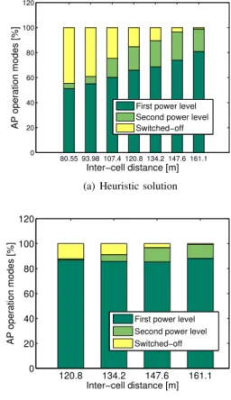
exam-ine the cause of power savings in the heuristic and the optimal solutions compared with Po-UA/HPL model forD ≤ 161.1 m, we plot Figures 3(a) and 3(b). These figures illustrate the percentage of the AP operation modes. For the heuristic solution, results are provided for D ranging between 80.6 m to 161.1 m. Whereas, for the optimal solution, results are provided for D ranging between 120.8 m to 161.1 m, as the optimal solution has high computational complexity for dense networks (i.e., D ≤ 120.8 m). We notice that in the heuristic solution, the percentage of switched-off APs and the percentage of APs transmitting at the second power level is greater than that in the optimal solution forD ranging between 120.8 m to 161.1 m. The reason for this is that the proposed heuristic has an aggressive power saving policy: it switches off iteratively the maximum number of possible APs then it reduces iteratively the transmit power level of the remaining possible APs, while associating users to the active APs in such a way to obtain in each iteration the minimum total

network delay. However, the optimization problem minimizes simultaneously the total network power and the total network delay. This explains why we obtain a solution where the total network power is higher than the heuristic one.

Moreover, for both (heuristic and optimal) solutions, we see that when D increases the percentage of switched off APs decreases, and the percentage of APs transmitting at the second power level increases. Precisely, for small values ofD (i.e., 80.6 m), the number of covering APs per UE is relatively high (i.e., 3.4 as shown in Table I); thus, a large number of APs can be switched-off or can transmit at low power level (i.e., 44% of the APs are switched-off as shown in Figure 3(a)). However, when the value of D increases, the number of covering APs per UE decreases and thus the possibility to switch off an AP or to transmit at low power level decreases in order to ensure coverage for all UEs in the network. This explains the increasing curves for the corresponding inter-cell distances in Figure 2. Also, this logic validate why we obtain in these solutions a total network power equals to the one in Po-UA/HPL model for large D (i.e., D ≥ 161.1 m) in the same figure. 80.55 93.98 107.4 120.8 134.2 147.6 161.1 0 20 40 60 80 100 120 Inter−cell distance [m] AP operation modes [%]

First power level Second power level Switched−off

(a) Heuristic solution

120.8 134.2 147.6 161.1 0 20 40 60 80 100 120 Inter−cell distance [m] AP operation modes [%]

First power level Second power level Switched−off

(b) Optimal solution

Figure 3. Percentage of AP operation modes in heuristic and optimal solutions.

We now investigate the total network delay for the heuristic and the optimal solutions compared with the Po-UA/HPL model while varying the inter-cell distance. The total network

80 100 120 140 160 180 200 220 0.4 0.6 0.8 1 1.2 1.4 1.6x 10 −4 Inter−cell distance [m]

Total network delay [s]

Po−UA/HPL

Power−Delay−Min (Optimal) Heuristic

Figure 4. Total network delay for heuristic and optimal solutions and for Po-UA/HPL.

delay is computed according to (5). As expected, Figure 4 shows that the Po-UA/HPL model has the lowest total network delay followed by the optimal solution and then by the heuristic solution. This is due to the fact that, in Po-UA/HPL model where all APs transmit at the highest power level, all UEs perceive a relatively high SNR which lowers the total network delay. However for the heuristic solution, the number of APs transmitting at low level or switched off is greater than that of the optimal one (as shown in Figure 3) and this causes the total network delay of the heuristic to be higher than the optimal one.

Moreover, we see that the total network delay for the optimal solution and for Po-UA/HPL model have increasing curves. Precisely, for the same UE distribution, whenD increases, the SNR of the UE decreases, thus the perceived rate decreases which causes the delay to increase. Whereas, the heuristic solution has a decreasing curve for D between 80.6 m and 161.1 m then it has an increasing one for D ≥ 161.1 m. Typically, for D between 80.6 m and 161.1 m, the number of APs transmitting at either the highest power level or the second power level increases (as shown in Figure 3(a)) and thereby UEs experience a lower delay.

Note that all the curves tend to converge to the same point. Precisely, for high values of inter-cell distance (D ≥ 161.1 m), the simulated algorithms converge to a solution where all APs transmit at the highest power level. This corresponds to the only feasible solution of the Power-Delay-Min problem. In this situation, this problem boils down to a user association problem that minimizes the sum of UE delays.

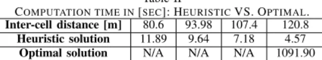
Finally, in order to study the computational complexity of the heuristic algorithm, we depict in Table II the average computation time of the heuristic and the optimal solutions as a function of the inter-cell distance. Results show that the heuristic solution has a low computational time for dense networks. For instance, forD equals 80.6 m, it takes 11.89 sec of computation time, whereas the optimal solution cannot be computed. Moreover, we notice that for D equals 128.08 m, the heuristic algorithm has a negligeable computation time compared to the optimal one. Furthermore, the computation time decreases when D increases. In fact, the complexity of executing the heuristic algorithm depends on the number of covering APs per user according to (11). As shown in

Table II

COMPUTATION TIME IN[SEC]: HEURISTICVS. OPTIMAL.

Inter-cell distance [m] 80.6 93.98 107.4 120.8

Heuristic solution 11.89 9.64 7.18 4.57

Optimal solution N/A N/A N/A 1091.90 Table I, when D increases, the number of covering APs per user decreases causing the computation time to decrease.

VII. CONCLUSION

In this paper, we proposed a novel heuristic algorithm for the joint Power-Delay minimization problem in WLANs. Our goal was to come-up with a heuristic that has low computational complexity and provides a satisfactory solution. Simulation results showed that the proposed heuristic gives comparable power savings with respect to an optimal solution. Moreover, for dense scenarios, the optimal solution is intractable whereas the heuristic algorithm provides efficient results that show significant power savings up to 45% compared with legacy networks in a reasonable time. However, for both solutions, the network power is saved at the cost of an increase in network delay. In addition, for sparse scenarios, there is no substantial gain compared with a reference model and thus power saving is superfluous. In future work, we seek to study the joint Power-Delay-Min problem for cellular networks considering 4G technology.

REFERENCES

[1] The benefits of centralization in wlans via the cisco unified wireless network. In Cisco Systems Inc., White paper, 2006.

[2] Channels and maximum power settings for cisco aironet lightweight access points. In Cisco Systems Inc., White paper, 2008.

[3] S. Chieochan, E. Hossain, and J. Diamond. Channel assignment schemes for infrastructure-based 802.11 wlans: A survey. IEEE Communications

Surveys Tutorials, 2010.

[4] O. J. Grodzevich and O. Romanko. Normalization and other topics in multi-objective optimization. In Workshop of the Fields MITACS

Industrial Problems, 2006.

[5] M. Heusse, F. Rousseau, G. Berger-Sabbatel, and A. Duda. Performance anomaly of 802.11b. In Proc. IEEE INFOCOM, 2003.

[6] M.F. Hossain, K.S. Munasinghe, and A. Jamalipour. A protocooperation-based sleep-wake architecture for next generation green cellular access networks. In Proc. International Conference on Signal Processing and

Communication Systems (ICSPCS), 2010.

[7] K. Khawam, M. Ibrahim, J. Cohen, S. Lahoud, and S. Tohme. Individual vs. global radio resource management in a hybrid broadband network. In

Proc. IEEE International Conference on Communications (ICC), 2011.

[8] J. Lorincz, A. Capone, and D. Begusic. Optimized network management for energy savings of wireless access networks. Computer Networks, 2011.

[9] F. Moety, S. Lahoud, K. Khawam, and B. Cousin. Joint Power-Delay minimization in green wireless access networks. In Proc. IEEE PIMRC, 2013.

[10] F. Richter, A. J. Fehske, and G. P. Fettweis. Energy efficiency aspects of base station deployment strategies for cellular networks. In Proc. IEEE

Vehicular Technology Conference Fall (VTC-Fall), 2009.

[11] K. Son, H. Kim, Y. Yi, and B. Krishnamachari. Base station operation and user association mechanisms for energy-delay tradeoffs in green cellular networks. IEEE Journal on Selected Areas in Communications, 2011.

[12] S. Tombaz, M. Usman, and J. Zander. Energy efficiency improvements through heterogeneous networks in diverse traffic distribution scenarios. In Proc. IEEE International ICST Conference on Communications and

Networking in China (CHINACOM), 2011.

[13] Y. Wu, G. He, S. Zhang, Y. Chen, and S. Xu. Energy efficient coverage planning in cellular networks with sleep mode. In Proc.

IEEE International Symposium on Personal Indoor and Mobile Radio