Combining Traffic Shaping Methods with Congestion Control Variants for HTTP Adaptive Streaming

HAL Id: hal-01249646

https://hal.archives-ouvertes.fr/hal-01249646

Submitted on 2 Jan 2016

HAL is a multi-disciplinary open access

archive for the deposit and dissemination of

sci-entific research documents, whether they are

pub-lished or not. The documents may come from

teaching and research institutions in France or

abroad, or from public or private research centers.

L’archive ouverte pluridisciplinaire HAL, est

destinée au dépôt et à la diffusion de documents

scientifiques de niveau recherche, publiés ou non,

émanant des établissements d’enseignement et de

recherche français ou étrangers, des laboratoires

publics ou privés.

Distributed under a Creative Commons Attribution - NonCommercial - NoDerivatives| 4.0

International License

Combining Traffic Shaping Methods with Congestion

Control Variants for HTTP Adaptive Streaming

Chiheb Ben Ameur, Emmanuel Mory, Bernard Cousin

To cite this version:

Chiheb Ben Ameur, Emmanuel Mory, Bernard Cousin. Combining Traffic Shaping Methods with

Congestion Control Variants for HTTP Adaptive Streaming. Multimedia Systems, Springer Verlag,

2018, 24 (1), pp.1 - 18. �10.1007/s00530-016-0522-9�. �hal-01249646�

1

Combining Traffic Shaping Methods with Congestion

Control Variants for HTTP Adaptive Streaming

Chiheb Ben Ameur

Orange Labs

Rennes, France

Chiheb.benameur@orange.com

Emmanuel Mory

Orange Labs

Rennes, France

emmanuel.mory@orange.com

Bernard Cousin

IRISA, University of Rennes 1

Rennes, France

Bernard.Cousin@irisa.fr

ABSTRACT

HTTP adaptive streaming (HAS) is a streaming video technique widely used over the Internet. However, it has many drawbacks that degrade its user quality of experience (QoE). Our investigation involves several HAS clients competing for bandwidth inside the same home network. Studies have shown that managing the bandwidth between HAS clients using traffic shaping methods improves the QoE. Additionally, the TCP congestion control algorithm in the HAS server may also impact the QoE because every congestion control variant has its own method to control the congestion window size. Based on previous work, we describe two traffic shaping methods, the Hierarchical Token Bucket shaping Method (HTBM) and the Receive Window Tuning Method (RWTM), as well as four popular congestion control variants: NewReno, Vegas, Illinois, and Cubic. In this paper, our objective is to provide a detailed comparative evaluation of combining these four congestion control variants with these two shaping methods. The main result indicates that Illinois with RWTM offers the best QoE without causing congestion. Results were validated through experimentation and objective QoE analytical criteria.

Keywords

Traffic shaping; Congestion control; Quality of Experience; HTTP Adaptive Streaming; Bandwidth management.

1. INTRODUCTION

HTTP adaptive streaming (HAS) is a streaming video technique based on downloading video segments of short duration. These segments are called chunks, and they are streamed from a HAS server to a HAS client through the network. Each chunk is encoded at multiple quality levels. After requesting a chunk by an HTTP GET request message, when the chunk is received, the player on the client side stores it in a playback buffer. The HAS player operates in one of two states: a buffering state and a steady state. During the first state, the player requests a new chunk as soon as a previous chunk has been downloaded, until the playback buffer is filled. However, during the steady state, the player requests chunks periodically in order to maintain a constant playback buffer size. The steady state includes periods of activity (ON periods) followed by periods of inactivity (OFF periods) [9], [11].

The Quality of Experience (QoE) of an HTTP adaptive stream depends primarily on three criteria:

1. Video quality level stability [1], [11]: A frequent change of video quality level bothers the user. Therefore, quality level fluctuation should be avoided to improve the QoE.

2. Fidelity to optimal quality level selection: The user prefers to watch the best video quality level, when possible. Therefore, the HAS player should select the optimal quality level, which is the highest feasible quality level allowed by the available bandwidth. 3. Convergence speed: The user prefers to view the

optimal quality level as soon as possible. Accordingly, the HAS player should rapidly select the optimal quality level. The delay that the player requires before the optimal quality level has been attained is called the convergence speed [1].

We studied a general use case in which several HAS clients are located in the same home network. In this use case, QoE degradations can be grouped into two main causes:

 Congestion events:

Video packets sent from the server to the client pass through many network devices. Each device has one or many queues that use a queuing discipline to schedule network packets. The implemented algorithm decides whether to route or drop incoming packets in order to avoid network congestion. The main bottleneck occurs near the home gateway, and more precisely, in the link between DSLAM and home gateway [12]. In fact, the DSLAM may considerably reduce the bandwidth offered to the home network, and it is more likely to drop packets than any other network device. To minimize network effects on the delivery, the TCP protocol implements a “congestion control algorithm” on the sender side, which reduces the bitrate of packets sent to the receiver when a packet is lost. However, this bitrate reduction may degrade QoE. In addition, there are many congestion control variants with different methods of managing the congestion window size,

cwnd, and detecting congestion events. These differences

may change the QoE between variants.

 Concurrence with other streams - OFF periods issue: The HAS player estimates the available bandwidth by computing the download bitrate for each chunk when it has

2 finished downloading; this is done by dividing the chunk size by its download duration. As a consequence, the player cannot estimate the available bandwidth during OFF periods, because no data are being received. When a HAS stream concurs with other streams in the same home network, accurate bandwidth estimation becomes more difficult. For example, when two HAS streams are competing for bandwidth and the ON period of the first player coincides with the OFF period of the second player, the first player will overestimate its available bandwidth. This overestimation may lead the player to select a higher quality level for the next chunk. This selection may lead to a congestion event and a resulting fluctuation of quality levels between the two players. Research has demonstrated that traffic shaping can considerably limit this problem [1, 2, 11, 21, 25]. Traffic shaping consists of selecting a target bitrate for each HAS session in the home network based on bitrates of the available quality levels and the available bandwidth. It then shapes the outgoing traffic to each HAS client based on the selected target bitrate.

The objective of our study is to combine two solution categories, TCP congestion control variants to reduce the negative effects of congestion events, and traffic shaping methods, to restrict the drawbacks of the concurrence between HAS streams in the home gateway. The optimal combination will have the highest grade of QoE, i.e. the best possible video quality level stability, best fidelity to optimal quality level selection, and best convergence speed. We note that there are many implementations of HAS that are currently deployed, such as Dynamic Adaptive Streaming over HTTP (MPEG-DASH), Microsoft Smooth Streaming (MSS), Apple HTTP Live Streaming (HLS), and Adobe HTTP Dynamic Streaming (HDS). For this reason, we wish to emphasize that in this paper we only choose HAS traffic shaping methods that do not change the HAS implementation either in the player or in the server. This choice provides adaptability to any HAS client or server implementations and thus offers a larger scope of application of our presented work.

The remainder of this paper is organized as follows. In Section 2, we describe the background and related works. In Section 3, we detail our methodology and experimental implementation. Section 4 presents the results and discussion. In Section 5, we conclude the paper and suggest future directions for our work.

2. BACKGROUND AND RELATED WORK

In this section, we describe the TCP congestion control variants and the HAS traffic shaping methods used in this work, and explain the distinctions between them.

2.1 TCP congestion control variants

All TCP congestion control variants have two common phases: a slow start phase and a congestion avoidance

phase. The slow start phase consists of increasing cwnd rapidly by one maximum segment size (MSS) for each received acknowledgment (ACK), i.e. the cwnd value is doubled for each round trip time (RTT). This rapidity has an objective of reaching a high bitrate within a short duration. When the cwnd size exceeds a threshold called ssthresh, the TCP congestion control algorithm switches to the second phase: the congestion avoidance phase. This phase slowly increases the cwnd until a congestion event is detected. TCP congestion control variants are classified according to two main criteria [13]:

1- The first criterion is the increase of cwnd during the congestion avoidance phase and the decrease of cwnd immediately following congestion detection. Generally, the increase is additive, and the cwnd size increases by one MSS for each RTT. For decreasing cwnd, the standard variants employ multiplicative decreasing, i.e. the cwnd size is weighted by a multiplicative decrease factor (1-β), where 0 < β < 1. This category is called the Additive Increase Multiplicative Decrease (AIMD) approach. Other variants using different techniques are classified as non-AIMD approaches.

2- The second criterion is the method by which the algorithm detects congestion. We distinguish three modes: loss-based, delay-based, and loss-delay-based modes. The loss-based mode considers any detection of packet loss as a congestion event. A majority of TCP congestion control variants that use the loss-based mode consider receiving three duplicated ACKs from the receiver as an indication of a packet loss and, as a consequence, as an indication of a congestion event. However, the delay-based mode considers a significant increase in the RTT value as the only indication of a congestion event. The third mode, the hybrid mode, combines the delay-based and loss-based modes to improve congestion detection.

In order to facilitate our study, we chose four well-known congestion control variants, and we classify them according to the two criteria cited above:

- NewReno [3]: This variant is designed as the standard TCP congestion control approach. It uses the AIMD approach with the loss-based mode. Two mechanisms are employed immediately following congestion detection: fast retransmit and fast recovery [14]. Fast retransmit consists of performing a retransmission of what appears to be the missing packet (i.e. when receiving 3 duplicate ACKs), without waiting for the retransmission timer to expire. After the fast retransmit algorithm sends this packet, the fast recovery algorithm governs the transmission of new data until a non-duplicate ACK arrives. The reason for using fast recovery is to allow the continual sending of packets when the receiver is still receiving packets, even if some packets are lost.

3

1: NewReno: ssthresh = max(cwnd/2, 2 MSS)

2: Vegas: ssthresh = min(ssthresh, cwnd - 1)

3: Illinois: ssthresh = max(cwnd.(1-β), 2 MSS)

4: Cubic: ssthresh = max(cwnd.(1-β), 2 MSS)

1: ssthresh = max(ssthresh, ¾ cwnd)

2: for i=1 to int(idle/RTO) do

3: cwnd = max ( min ( cwnd , rwnd )/2, 1 MSS )

4: end for - Vegas [4]: This non-AIMD variant is an Additive

Increase Additive Decrease (AIAD) variant. It is a delay-based variant that accurately estimates RTT for every sent packet and adjusts cwnd size based on actual throughput and expected throughput. If RTT increases, cwnd decreases by one MSS, and vice versa. Vegas is the smoothest TCP congestion control variant [15]; it is able to allocate a fair share of bandwidth with minimal packet loss events. - Illinois [5]: This is a TCP loss-delay-based congestion variant that employs a particular classification of the AIMD approach, C-AIMD, which involves a concave window size curve. Packet loss is used for primary congestion inference to determine the direction (increase or decrease) of cwnd, with a delay for secondary congestion inference to adjust the value of the window size change. More precisely, when the average queueing delay is small (small increase of

RTT), the sender supposes that the congestion is not

imminent and specifies a large additive increase α and small multiplicative decrease β. In the opposite case, when the average queuing delay is large (large increase of RTT), the sender supposes that the congestion is imminent and selects a small α and large β. Illinois measures RTT for each received ACK to update α and β. Moreover, it retains the same fast recovery and fast retransmit phases as NewReno. Illinois was designed for high-speed and high-latency networks, where the bandwidth-delay product is relatively high. Consequently, it enables higher throughput than NewReno.

- Cubic [6]: This variant is loss-based, but it uses a non-AIMD approach. A cubic function is used to increase the

cwnd in the congestion avoidance phase immediately after

the fast recovery phase, and a multiplicative decrease approach is used to update the cwnd after congestion event detection. The cubic function has a concave region followed by a convex region. The plateau between the two regions, or the inflexion point (denoted by Wmax), corresponds to the window size just before the last congestion event. The cubic function enables a slow growth around Wmax to enhance the stability of the bandwidth, and enables a fast growth away from Wmax to improve scalability of the protocol. Upon receiving an ACK during the congestion avoidance phase at time t, Cubic computes the new value of cwnd corresponding to the cubic function at time t. As a consequence, Cubic uses the time instead of the RTT to increase the cwnd. Cubic employs a new slow-start algorithm called HyStart [8] (hybrid slow slow-start), which finds a safe exit point to the slow start, the ssthresh value, at which the slow start can finish and safely move to congestion avoidance before cwnd overshoot occurs. HyStart employs the RTT delay increase and the inter-arrival time between consecutive ACKs to identify the safe exit point, and to modify the ssthresh value [8]. This variant does not make any change to the fast recovery and fast retransmit of standard NewReno. Cubic is the smoothest

loss-based congestion control variant [15]: it is characterized by a congestion window that falls less abruptly and that remains constant over a wide range of elapsed time. It is also designed for speed and high-latency networks.

For precise analysis, based on the descriptions of congestion control algorithm variants and their source code, we describe below the update of the congestion window size, cwnd, and the slow start threshold value, ssthresh, for different events:

- Congestion events: there are two cases

o When a congestion event is detected, the Fast Recovery / Fast Retransmit (FR/FR) phase reduces the ssthresh value and sets the cwnd value to

ssthresh+3, for the purpose of remaining in the

congestion avoidance phase. The ssthresh value after a congestion event is updated as follows:

Algorithm 1 ssthresh update after a congestion event

where MSS is the maximum segment size, and β is the multiplicative decrease factor.

o When the retransmission timeout expires before receiving any ACK of the retransmitted packet,

ssthresh is reduced as indicated in Algorithm 1 , and cwnd is set to a small value and restarts from the

slow start phase.

- Idle period: When the server sends a packet after an idle period that exceeds the retransmission timeout (RTO),

cwnd and ssthresh are computed for the four

congestion control variants as in Algorithm 2:

Algorithm 2 cwnd and ssthresh updates after idle period

In the HAS context, an idle period coincides with an OFF period between two consecutive chunks. An OFF period whose duration exceeds RTO is denoted by OFF*.

Furthermore, we additionally want to emphasize that the rate of a TCP connection can be approximated, if we assume that transients due to slow start and fast recovery can be neglected, by [26], where

rwnd is the TCP receive window indicated by the receiver

and RTT is the round trip time between the sender and the receiver. Obviously, this approximation is valid for the four TCP congestion control variants described above. As we have shown, these variants employ different algorithms to modify the congestion window, cwnd, during the congestion avoidance phase and after congestion detection.

4 Accordingly, the generated rate as well as its variation over time are different from one variant to another.

2.2 Traffic shaping methods

Many studies have been conducted to improve HAS performance for cases in which several HAS clients are located in the same home network. The ON-OFF periods characterizing the HAS player in its steady state involve three substantial problems when HAS players are competing: player instability, unfairness between players, and bandwidth underutilization [9]. The cause of these problems is the inability to estimate the available bandwidth during the OFF period, because no data are being received. Three types of solutions are proposed to improve HAS user experience: client-based, server-based, and gateway-based solutions. They differ with respect to the device in which the shaping solution is implemented. Below, we cite relevant methods for each type of solution:

- The client-based solution involves only the HAS client in order to reduce its OFF period durations. One of the recent client-based methods is proposed in the FESTIVE method [7]. It randomizes the events of chunk requests inside the player in order to reduce the periodicity of ON periods. Consequently, most of the incorrect estimations of bandwidth could be avoided when several HAS clients compete for bandwidth. However, this method is not efficient enough to prevent all incorrect estimations. In addition, it modifies the HAS player implementation, which is contradictory to our specifications described in the Introduction. Moreover, the client-based solution does not provide the coordination between HAS clients that is required to further improve bandwidth estimations and QoE.

- The server-based solution involves only the HAS server. It proceeds according to two steps: First, finding the optimal quality level for each provided HAS flow, and second, shaping the sending rate of the HAS server according to the encoding rate of this level. In [25], the authors propose a server-based method: it consists in detecting the oscillations between quality levels on the server side and deciding which optimal quality level must be selected. Although this method improves the QoE, it cannot conveniently respond to the typical use cases of several concurrent HAS clients that do not share the same HAS server: the shared link is on the HAS client side. Moreover, this server-based solution requires an additional processing task, which becomes burdensome and costly when many HAS clients are demanding video contents from the same HAS server. In addition, the server-based solution is unable to acquire information about the other competing flows with their corresponding HAS clients. Hence, the selection of the optimal quality level at the

server is a vague estimation. This estimation is less accurate than a quality level selection based on a sufficient knowledge about the access network of the corresponding HAS client(s).

- The gateway-based solution that consists of applying the HAS traffic shaping in the gateway is more convenient than client-based and server-based solutions; in fact, the gateway can acquire information about the HAS traffic of all clients of the same home network, which is not possible either at the server or at the client. In addition, the gateway-based solution is able to perform traffic shaping without inducing any modification of HAS implementation code either in the server or the client. Hence, in this paper, our evaluations only consider the gateway-based shaping solution. For the gateway-based solution, the authors assumed that the home gateway can intercept the manifest file during the HAS session initialization and can obtain the characteristics of the available video quality levels of every session. This solution introduces a bandwidth manager in the gateway that defines a shaping rate for each connected active HAS client in the home network. The bandwidth manager should be able to update the number of active connected HAS clients in the home gateway by sniffing the SYN and FIN flags in TCP packets. Therefore, the difference between the gateway-based methods is the manner in which they shape the bandwidth for each HAS session. The two main gateway-based methods found in the literature and used in our comparative study are HTBM [1] and RWTM [2]. They are briefly described in the following:

2.2.1 HTBM

HTBM uses the Hierarchical Token Bucket (HTB) queuing discipline to shape the HTTP adaptive streams. HTB is integrated in Linux with the traffic controller tool of the

iproutes2 utility package. It uses one link, designated as the

parent class, to emulate several slower links, designated as the children classes. Different types of traffic may be served by the emulated links. HTB is exploited by the bandwidth manager of HTBM in order to define a child class for each HAS session. HTB also employs the tokens and buckets concept, combined with the class-based system for better control over traffic and for shaping in particular [16]. A fundamental component of the HTB queuing discipline is the borrowing mechanism: children classes borrow tokens from their parent once they have exceeded the shaping rate. A child class will continue to try to borrow until it reaches a defined threshold of shaping, at which point it will begin to queue packets that will be transmitted when more tokens become available.

Accordingly, using HTBM enables the shaping of the HTTP adaptive streams for each HAS session in the gateway, as indicated by the bandwidth manager, by merely

5 delaying packets that are received from the HAS server. The authors of [1] indicate that HTBM improves the user’s QoE; it improves the stability of video quality level, the fidelity to optimal quality level, and the convergence speed.

2.2.2 RWTM

The second shaping method, Receive Window Tuning Method (RWTM), is a gateway-based shaping method that was proposed in [2]. It is implemented in the TCP layer and is based on TCP flow control at the receiver side. Indeed, during a TCP session, each receiver specifies the maximum number of bytes that it is able to buffer. This value is called the receiver’s advertised window, denoted by rwnd, and its size is specified in the rwnd field in the header of each TCP packet sent from the receiver to the sender. The sender receives the rwnd size from the receiver and limits its sending window, W, so that the number of packets sent in each RTT does not exceed rwnd; W=min(rwnd, cwnd). The RWTM method consists of modifying, in the gateway, the rwnd field of each TCP ACK packet sent from a HAS client C to its HAS server S in order to limit the sending rate of the HAS server to rwnd/RTTC-S. RWTM uses the

defined shaping rate of the bandwidth manager for each connected active HAS client, and estimates the RTTC-S value

to compute the next value of rwnd. We note that the estimation of RTTC-S is accomplished using only TCP ACK

packets sent from HAS clients to the HAS server by using passive estimation. The rwnd is computed once for each ON period. RWTM was tested in [2] and [21], and results indicated that RWTM enhances the user’s QoE: it improves the stability, the fidelity, and the convergence speed. In [21], we showed that RWTM outperforms HTBM when using the Cubic variant as congestion control on the server side. However, due to the dissimilarity of TCP variants, an extended evaluation using other variants and additional scenarios will give us a better understanding of the interaction between shaping methods and TCP variants.

3. METHODOLOGY AND

EXPERIMENTAL IMPLEMENTATION

In this section, we provide a description of the metrics used to measure performance, the scenarios that cover many operating conditions, and the framework that has been developed to emulate our use case.

3.1 Performance metrics

We define three metrics in this section that we use to evaluate the QoE and to understand how each combination behaves. To do so, we present in Table 1 the main parameters that are used to define the metrics.

Table 1. Description of parameters

Parameter Description

i Discrete time index

LC(i) Video quality level index of client C at time i. LC,opt(i) Theoretical optimal value of LC(i)

QC(i) Video encoding bitrate of client C at time i

We note that the optimal quality level value, LC,opt(i), corresponds to the quality level that the client C should select at time i under the shaping rate defined by the bandwidth manager. This shaping rate is chosen in a manner that ensures the fairest share of the available home bandwidth between clients with prioritization to achieve the maximum use of the available home bandwidth. This entails that some clients could have a higher quality level than others when their fair share of available home bandwidth is not sufficient to maximize the use of the available home bandwidth. Below, we define analytically three performance metrics that describe the three criteria of QoE mentioned in the Introduction:

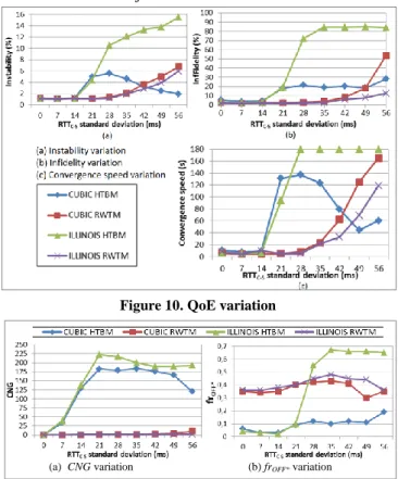
3.1.1 Video quality level stability

Many research studies indicate that HAS users are likely to be sensitive to frequent and significant quality level switches [22, 23]. We use the instability metric, , which measures the instability for client C for a K-second test duration in conformity with its description in [7] as the following equation: is the weighted sum of all encoding bitrate switching steps observed within the last K seconds divided by the weighted sum of the encoding bitrates selected in the last K seconds. The lower the value is, the higher the stability of the video quality level is.

More precisely, this formula uses the encoding bitrates of the selected quality levels over time, , instead of the quality level index over time, . In fact, the absolute difference between two encoding bitrates that are displayed on the client side during two successive seconds, and , and denoted by , gives more significant indication of the observed video quality change than when using the absolute difference between the quality level indexes. Hence, we can offer an adequate representation of the user expectation.

Moreover, in this formula, the authors of [7] use the weight function in order to add a linear penalty to more recent quality level switches. In fact, their justification is that the switching of quality level is becoming more disturbing for users’ experience when the video playback position is far from the beginning of the video stream.

3.1.2 Fidelity to optimal quality level

In [7], the authors define two additional goals to achieve within our use case: 1) fairness between players: players should be able to converge to an equitable allocation of network resources; 2) efficiency among players: players should choose the highest feasible quality levels to maximize the user’s experience. Furthermore, in [9], the authors address the bandwidth underutilization issue that may prevent the possible improvement of QoE. So,

6 maximizing the use of bandwidth can be considered as a QoE criterion. Accordingly, in order to provide one formula that satisfies these three criteria, we define our metric called

infidelity to optimal quality level.

The infidelity metric, of client C for a K-second test duration, measures the duration of time over which the HAS client C requests optimal quality:

The lower the value is, the higher the fidelity to optimal quality is.

Here, we note that the theoretical optimal quality level

aims to resolve the dilemma between the two

criteria of maximum use and fair share of bandwidth between HAS players. In fact, considering that only the fair share of bandwidth may cause bandwidth underutilization, in some cases it may leave some residual bandwidth allocated to nobody. Hence, based on the optimal quality level, the value of the infidelity metric is representative of user expectation.

3.1.3 Convergence speed

The convergence speed metric was previously defined in [1]. We provide an analytical definition as follows:

This metric is the time that the player of HAS client C takes to reach and remain at the optimal quality level for at least T seconds during a K-second test duration. The reason of selecting this criterion for evaluating the QoE in our use case is observations made in [1], [2], [9], and [21]: they show that when HAS players compete for bandwidth, the convergence to optimal quality level may take several seconds or may be very difficult to be achieved. Accordingly, the speed of this convergence is a valuable QoE criterion for our evaluations. The lower the

value is, the faster the convergence to the optimal quality level is.

Additionally, we define two other metrics (CNG and frOFF*,

described below) that enable us to measure the reaction of home gateway and HAS players.

3.1.4 Congestion rate

The congestion detection events influence to an extreme degree both the QoS and QoE of HAS because the server decreases its sending rate after each congestion detection. Hence, by analyzing the code description of the four TCP congestion control algorithms (NewReno, Vegas, Illinois, and Cubic), we found that the congestion event appears when the value of parameter slow start threshold (ssthresh) decreases (see Algorithm 1). Hence, we define a metric called congestion rate, denoted by , that

computes the rate of congestion events that are detected on the server side, corresponding to the HAS flow between client C and server S during a K-second test duration as shown in equation

(4):

where is the number of times the ssthresh has

been decreased for the C-S HAS session during the K-second test duration.

3.1.5 Frequency of OFF* periods per chunk

This metric is important to measure the frequency of OFF* periods. An OFF period whose duration exceeds RTO is denoted by OFF* (as indicated in Subsect. 2.1). This frequency is equal to the total number of OFF* periods divided by the total number of downloaded chunks. This metric is denoted by frOFF*.

For result analysis, we use the QoE metrics to quantitatively discuss the user’s experience, and use CNG and frOFF*

metrics to explain the performance of each combination of traffic method and congestion variant.

3.2 Scenarios

We define five scenarios that are typical of concurrence between HAS clients in a same home network (scenarios 1, 2, and 3), and how the HAS client reacts when some changes occur (scenarios 4 and 5):

1. Both clients start to play simultaneously and continue for 3 minutes. This scenario illustrates how clients compete.

2. Client 1 starts to play, the second client starts after 30 seconds, and both continue together for 150 seconds. This scenario shows how the transition from one client to two clients occurs.

3. Both clients start to play simultaneously, client 2 stops after 30 seconds, and client 1 continues alone for 150 seconds. This scenario shows how a transition from two clients to one takes place.

4. Only one client starts to play and continues for 3 minutes. At 30 seconds, we simulate a heavy congestion event with a provoked packet loss of 50% of the received packets at the server over a 1-second period. This scenario shows the robustness of each combination against the congestions that are induced by external factors, such as by other concurrent flows in the home network.

5. Only one client is playing alone for 3 minutes. We vary the standard deviation value of RTTC-S (round trip time

between the client and the server) for each set of tests. This scenario investigates the robustness against RTTC-S

instability.

The test duration was selected to be 3 minutes to offer sufficient delay for players to stabilize.

7

3.3 General framework

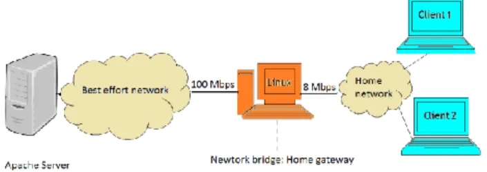
We propose a testbed architecture presented in Figure 1 that emulates our use case described in the Introduction. The choice of only two clients is sufficient to show the behavior of concurrence between many HAS flows in the same home network.

Figure 1. Architecture of the testbed

In this section, we describe the configurations of each component presented in Figure 1:

- HAS clients

We used two Linux machines as HAS clients. We developed an emulated player in each client that reproduces the behavior of the HAS player without decoding and displaying a video stream. The playback buffer size is specified to be 15 chunks, and the chunk duration is 2 seconds. In [18], the authors indicate that the bitrate adaptation algorithm depends on bandwidth estimation and playback buffer occupancy. Furthermore, players also define an aggressiveness level, as described in a previous study [19]. For example, the Netflix player is more aggressive than the Smooth Streaming player [19]. An aggressive player enables the user to ask for a video quality level that is slightly higher than the estimated available bandwidth. Moreover, aggressiveness is important for minimizing the “downward spiral effect” phenomenon [20]. This phenomenon consists of underestimating the available bandwidth, which leads to a lower video quality level selection. Accordingly, taking into consideration [18], [19], and [20], we used a bitrate adaptation algorithm based on bandwidth estimation in which we define an aggressiveness

ρC(t) at time t that depends on playback buffer occupancy as

follows:

ρC(t) = σ.RC(t)/BC (5)

where RC(t) is the filling level of the playback buffer at time

t, BC is the size of the playback buffer of client C, and σ is

the aggressiveness constant. The fuller the playback buffer is, the closer to σ the aggressiveness is.

All tests use a HAS player with an aggressiveness constant of σ=0.2. This enables the HAS player to add a maximum of 20% to its available BW estimation.

- Home network

In the modeled home network, the clients are connected directly to the gateway. The total download bitrate, or home available bandwidth, is limited to 8 Mbps. We choose this value because it is lower than twice the video encoding bitrate of the highest quality level. Accordingly, two clients

in the home network cannot select the highest quality level at the same time. In this case, one client should select quality level n° 4 and the other should select the quality level n° 3as optimal qualities. We do not test a use case in which two clients have the same optimal quality level, because this is a very specific case, and dissimilarity between optimal quality levels is more general.

- Home gateway

The emulated home gateway consists of a Linux machine configured as a network bridge to forward packets between the home network and the best effort network.

We emulate the queuing discipline of the home gateway by using the Stochastic Fairness Queueing discipline (SFQ) [24]. SFQ is a classless queuing discipline that we configured using the Traffic Controller emulation tool (tc). SFQ schedules packets based on flow identification (the source and destination IP addresses and the source port) and injects them into hash buckets during the enqueuing process. Each bucket represents a unique flow. Additionally, SFQ employs Round Robin fashion for dequeuing packets by taking into consideration the bucket classification. The goal of using buckets for enqueuing and Round Robin for dequeuing is to ensure fairness between flows so that the queue is able to forward data in turn and prevents any single flow from drowning out the remaining flows. We also configured SFQ in order to support the Drop Tail queue management algorithm when the queue becomes full. Hence, this configuration of the queuing discipline is classified as a Drop Tail class. The queue length of SFQ, which is indicated by parameter limit within the tc tool, is set to the bandwidth-delay product.

In the gateway, we implemented a bandwidth manager that selects a shaping rate for each connected active HAS client in a manner such that each client should attain its optimal quality level described in Subsect. 3.1. The shaping rate for each client was chosen as indicated in [1] and [2]; it is 10% higher than the encoding bitrate of the optimal quality level for each client. The two shaping methods HTBM and RWTM are implemented in the gateway, and they shape bandwidth in accordance with the decisions of the bandwidth manager.

- Best effort network

The best effort network is characterized by the presence of network devices to route packets. The round trip time RTT C-S(t) in a best effort network is modeled as follows [10]:

RTTC-S (t) = aC-S + q(t)/ς (6)

where aC-S is a fixed propagation delay between client C

and server S, q(t) is the queue length of a single congested router (the home gateway in our use case), and ς is the transmission capacity of the router. q(t)/ς models the queuing processing delay. To comply with equation (6), we used the normal distribution with a mean value aC-S and a

8 deviation emulates the queuing processing delay q(t)/ς. This emulation is accomplished by using the “netem delay” parameter of the traffic controller tool in the gateway machine interface.

- HAS server

The HAS server is modeled by an HTTP Apache Server installed on a Linux machine operating on Debian version 3.2. We can change the congestion control variant of the

server by varying the parameter

net.ipv4.tcp_congestion_control. All tests use five video

quality levels denoted by 0, 1, 2, 3, and 4. Their encoding bitrates are constant and equal to 248 kbps, 456 kbps, 928 kbps, 1,632 kbps, and 4,256 kbps, respectively. HTTP version 1.1 is used to enable a persistent connection.

4. RESULTS

In this section, we compare the different combinations of TCP congestion control variants in the server and shaping methods in the gateway in the five scenarios. Altogether, we evaluate eight combinations: four TCP congestion control variants combined with two shaping methods. We evaluate QoE by discussing the QoE metrics IS, IF, and V. We also use the CNG and frOFF* metrics to observe how each

combination reacts. For each scenario, we repeated each test 60 times and we computed an average value of each metric. The number of 60 runs is justified by the fact that the difference of the average results obtained after 40 runs and 60 runs are lower than 6%. This observation was verified for all scenarios. Accordingly, 60 runs are sufficient to achieve statistically significant results.

This section is organized as follows. First, we begin by evaluating performance in scenario 1, and we analyze the variation of cwnd for each combination. Second, we evaluate the performance of scenarios 2 and 3 to study the effect of transition from one to two clients (and vice versa) on the performance of each studied combination. Third, we present the performance of scenario 4 to measure the robustness of the combinations against induced congestions. Fourth, we study scenario 5 to measure the robustness against the instability of RTTC-S for each combination.

Finally, we discuss all results by presenting a summary of observations and defining the combination that is suitable for each particular case.

4.1 Scenario 1

In this scenario, two clients are competing for BW and are playing simultaneously. The available home bandwidth permits only one client to have the highest quality level, n° 4. We make the assumption that the client who gets the highest quality level n° 4 is identified as client 1. Optimally, the first player in our use case should obtain quality level n° 4 with an encoding bitrate of 4,256 kbps, and the second player should have quality level n°3 with an encoding bitrate of 1,632 kbps.

In this section, we present our evaluation results and discuss them. Then, we analyze the cwnd variation for each combination in order to understand the reason for the observed results.

4.1.1 Measurements of performance metrics

The average values of QoE metric measurements for client 1 and client 2 are listed in Tables 2 and 3, respectively.

Table 2. QoE for client 1 in scenario 1

Performance metric

Shaping method

TCP congestion control variant NewReno Vegas Illinois Cubic Instability (%) IS1(180) W/o* 4.95 2.15 8.35 7.47 HTBM 1.89 1.08 1.56 1.86 RWTM 1.69 4.10 1.88 1.63 Infidelity (%) IF1(180) W/o 41.33 52.31 74.14 50.46 HTBM 49.57 47.81 7.75 20.45 RWTM 45.87 32.24 6.17 5.02 Convergence speed (s) V1,60(180) W/o 100.93 102.11 174.13 145.03 HTBM 101.83 87.11 21.10 52.06 RWTM 94.51 104.00 24.22 19.55

Table 3. QoE for client 2 in scenario 1

Performance metrics

Shaping methods

TCP congestion control variants NewReno Vegas Illinois Cubic

Instability (%) IS2(180) W/o 5.82 3.06 7.85 5.82 HTBM 1.17 0.95 1.05 1.15 RWTM 1.09 0.95 1.03 1.13 Infidelity (%) IF2(180) W/o 26.64 70.77 39.27 36.33 HTBM 4.72 3.62 4.21 4.47 RWTM 2.49 2.30 2.47 2.61 Convergence speed (s) V2,60(180) W/o 96.25 137.01 126.33 92.81 HTBM 12.41 6.95 9.73 13.26 RWTM 6.73 5.03 6.54 8.95

Our first overall observation is the large dissimilarity between QoE measurements of the different combinations. This observation is a valuable result that confirms that each combination induces a change of HAS player behavior. Consequently, using HAS traffic shaping without taking into consideration the TCP congestion control employed in the HAS server cannot guarantee a good user experience; hence, the prominence of our proposed work.

The results show that traffic shaping considerably improves the QoE metric measurements for a majority of cases, especially for instability, which is largely reduced (e.g. a reduction of instability rate by a factor of 2.6 from 4.95% to 1.89% when employing HTBM with NewReno, and a reduction by a factor of 4.5 from 7.47% to 1.63% when employing RWTM with Cubic, as shown in Table 2). Furthermore, RWTM shows better performance than HTBM in the majority of cases. Moreover, client 2 always has better performance than client 1 with both shaping methods: the reason is that the optimal quality level of client 2 (i.e. quality level n° 3) is lower than that of client 1 (i.e. quality level n° 4): obviously, the quality level n° 3 is easier to achieve. In addition, the gap between the QoE metric measurements of the two shaping methods is higher for client 1 than client 2: For example, when considering the Cubic variant, the gap of infidelity rate of client 1 between RWTM and HTBM is 15.43% (5.02% vs.

9 20.45%); this is higher than that of client 2, which is equal to 1.86% (2.61% vs. 4.47%). Consequently, the dissimilarity of performance between different combinations is more visible for client 1. For this reason, we limit our observation to client 1 in the remaining text of this subsection.

Concerning the QoE measurements, based on Table 2, we present the most important observations related to client 1:

 Combining NewReno or Vegas variants with HTBM or RWTM does not improve the QoE. Additionally, these four combinations have high infidelity value (near 50%) and very high congestion speed value (around 90 ~100 ms), but a low value of instability. These values indicate that the player was stable at a low quality level during the first half of the test duration and has difficulties converging to its optimal quality level.

 HTBM has better QoE with Illinois than with Cubic: it is slightly more stable, 16% more faithful to optimal quality, and converges 2.4 times faster.

 RWTM has better QoE with Cubic than with Illinois: it is slightly more stable, slightly more faithful to optimal quality level, and converges 1.24 times faster.

In order to be more accurate in our analysis, we use the two defined metrics: the frequency of OFF* periods per chunk,

frOFF*, and the congestion rate, CNG. In Table 4, we present

the average value over 60 runs for each metric and for each combination, related to client 1 and scenario 1.

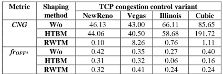
Table 4. frOFF* and CNG for client 1 in scenario 1 Metric Shaping

method

TCP congestion control variant NewReno Vegas Illinois Cubic

CNG W/o 46.13 43.00 66.11 85.65 HTBM 44.06 40.50 58.68 191.72 RWTM 0.10 8.26 0.76 1.11 frOFF* W/o 0.42 0.35 0.27 0.40 HTBM 0.31 0.32 0.06 0.16 RWTM 0.32 0.41 0.24 0.24

RWTM presents a negligible congestion rate, while HTBM has a very high rate of congestion, especially when the Cubic variant is used. Moreover, HTBM reduces the frequency frOFF* better than RWTM, mainly with Illinois

and Cubic. These results have a direct relationship to the shaping methods described in Subsect. 2.2:

 HTBM was designed to delay incoming packets, which causes an additional queuing delay. In all of the tests, we verified that HTBM induces a queueing delay of around 100 ms in scenario 1 for client 1. On one hand, this delay causes an increase of congestion rate because it increases the risks of queue overflow in the gateway, even when the QoE is good, such as with Cubic or Illinois variants. The dissimilarity of congestion rate between congestion controls variants is

investigated in the next Subsect. 4.1.2. On the other hand, the RTTC-S value also jumps from 100 ms to 200 ms, which increases the retransmission timeout value, RTO, to approximately 400 ms, hence reducing OFF* periods. The frOFF* of

HTBM is noticeably lower than RWTM and the case without shaping (W/o). In addition, the assertion “the higher the QoE metric measurement, the lower the frOFF* value” seems to be valid; for

example, HTBM presents better QoE with Illinois than with Cubic, and frOFF* is lower with Illinois

than with Cubic.

 Nevertheless, RWTM was designed to limit the value of the receiver’s advertised window, rwnd, of each client. Therefore, no additional queuing delay is induced by RWTM. Hence, the congestion rate is very low. Additionally, the RTTC-S

estimation is performed only once per chunk. So, the cwnd value is constant during the ON period, even if RTTC-S varies. In our configuration, the

standard deviation of RTTC-S is equal to 7 ms, i.e.

0.07.aC-S, as described in Subsect. 3.3. Consequently, eliminating OFF* periods will not be possible. Instead, the frOFF* value will be

bounded to a minimum value that characterizes RWTM when the QoE measurements are the most favorable. When testing with the four congestion control variants, this frOFF* value is equal to 0.24

for the selected standard deviation. This means that RWTM can guarantee, in the best case, one

OFF* period every 4.17 chunks. This frequency is

useful, and will be discussed in the next subsection and in further detail in scenario 5.

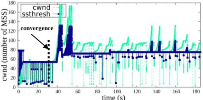
4.1.2 Analysis of cwnd variation

To explain the results of scenario 1, we used the tcp_probe module in the HAS server. This module shows the evolution of the congestion window, cwnd, and the slow start threshold, ssthresh, during each run. For each combination, we selected a run the performance values of which are the nearest to its average values of Tables 2 and 4, i.e. instability IS, infidelity IF, convergence speed V, frequency of OFF* periods per chunk frOFF*, and

congestion rate CNG. Then, we present their cwnd and

ssthresh evolution in Figures 2 through 9. We also indicate

the moment of convergence by a vertical bold dotted line. We observed that this moment corresponds to the second from which the TCP congestion control is often processing under the congestion avoidance phase; i.e. when cwnd >

ssthresh. In addition, from the moment of convergence, we

observe that ssthresh becomes more stable and is practically close to a constant value.

Figure 2 shows that the combination NewReno with HTBM cannot guarantee convergence to the optimal quality level. The congestion rate is not very high compared with other

10 TCP congestion variants. After 50 seconds, cwnd was able to reach the congestion avoidance phase for short durations, but the continuous increase of cwnd with the additive increase approach caused the detection of congestion. Moreover, the multiplicative decrease approach after congestions employed by NewReno was very aggressive; in effect, as described in Subsect. 2.2, the new cwnd value will be reduced by half (more precisely, to cwnd/2 + 3 MSS following the FR/FR phase) and ssthresh will also be reduced to cwnd/2. This aggressive decrease prevents the server from rapidly reaching a desirable cwnd value and, as a consequence, prevents the player from correctly estimating the available bandwidth and causes a lower quality level selection. Furthermore, the frOFF* value was

relatively high (around 0.3 OFF* period per chunk), which is more than twice that of the Illinois and Cubic variants. This value is also caused by the multiplicative decrease approach that generates a lower quality level selection. Due to the shaping rate that adapts the download bitrate of the client to its optimal quality level, the chunk with a lower quality level will be downloaded more rapidly, which results in causing more frequent OFF* periods. For this reason, the player was not able to stabilize on the optimal quality level, resulting in a poor QoE.

Figure 2. Cwnd variation of {NewReno HTBM}

IS=5.48%, IF=35.68%, V=180s, frOFF*=0.2, CNG=43.33

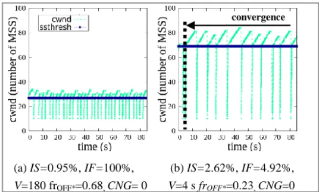
When combining NewReno with RWTM, we observed that test results diverged and could be classified into two categories: those with an infidelity value of 100% and that do not converge (Figure 3(a)), and those with a low value of infidelity and that converge rapidly (Figure 3(b)). In both figures, ssthresh is always invariable. Both figures have no congestion events, which is due to the use of RWTM.

(a) IS=0.95%, IF=100%, (b) IS=2.62%, IF=4.92%,

V=180 frOFF*=0.68, CNG= 0 V=4 s frOFF*=0.23, CNG=0

Figure 3. Cwnd variation of {NewReno RWTM}

The OFF* periods are more frequent in Figure 3(a) (frOFF*

= 0.68) than in Figure 3(b) (frOFF* = 0.23). Although both

figures present a constant value of ssthresh, we observe that the only difference between them is the initial value of

ssthresh. Figure 3(a) has a lower value of ssthresh than

Figure 3(b): 27 MSS vs. 69 MSS. The additive increase approach of NewReno during the congestion avoidance phase prevents the server from rapidly increasing the cwnd value during ON periods. Therefore, the player was not able to reach the optimal quality level n° 4 at any time. The cause of the dissimilarity between the initial values of

ssthresh in the two figures is explained in [17]. Some

implementations of NewReno use the size of the receiver’s advertised window, rwnd, to define the initial value of

ssthresh, but in fact, this value may be arbitrarily chosen.

Accordingly, the combination of NewReno with RWTM could have high QoE if the initial value of ssthresh is well-chosen.

When combining Vegas with HTBM, we obtain a cwnd variation, as shown in Figure 4. The convergence moment (at 87 s in Figure 4) occurs when cwnd becomes often set higher than ssthresh (i.e. TCP congestion control is often processing under the congestion avoidance phase) and

ssthresh is often set at the same value. We can observe the

additive increase and additive decrease aspect of cwnd in the congestion avoidance phase after convergence. The additive decrease of cwnd involved in Vegas is caused by the queuing delay increases resulting from HTBM. This additive decrease has the advantage of maintaining a high throughput and reducing the dropping of packets in the gateway. Therefore, the congestion rate, CNG, is relatively low because it is reduced in Figure 4 from around 75 congestion events per 100 seconds to only 15. The additive decrease also has the advantage of promoting convergence to the optimal quality level, unlike multiplicative decrease. As a result, the delay-based aspect with the additive decrease approach improves the stability of the HAS player after convergence. In contrast, Vegas uses a slightly low value of ssthresh (60 MSS) and employs the additive increase approach for cwnd updates during the congestion avoidance phase. As a consequence, the server cannot rapidly increase the cwnd value during the ON period, which results in slow convergence. Therefore, the player

Figure 4. Cwnd variation of {Vegas HTBM}

IS=1.31%, IF=46.74%, V=87 s, frOFF*=0.4, CNG=46.11

convergence convergence

11 was not able to reach the optimal quality level n° 4at any time before the moment of convergence. Consequently, the frequency of the OFF* period increases before the convergence moment; hence, the high value of frOFF*.

The performance worsens when Vegas is combined with RWTM. As presented in Figure 5, the player was not able to converge. Instead, we observed many timeout retransmissions characterized by ssthresh reduction and

cwnd restarting from slow start. The timeout retransmissions are generated by Vegas when only a duplicate ACK is received and the timeout period of the oldest unacknowledged packet has expired [4]. Because of that, Vegas generates more timeout retransmissions than NewReno. Hence, the CNG value is worse than in the other combinations of RWTM. Moreover, OFF* periods are frequent during the first 45 seconds, because the player requests quality level n° 3. Subsequently, OFF* periods become less frequent (they occur only at 79, 125, 138, 150, 165, and 175 s) because the player was able to switch to an optimal quality level (n° 4). Hence frOFF* related to the

whole test duration is equal to an acceptable value (0.29

OFF* period per chunk). The player becomes able to

request the optimal quality level n° 4 predominantly in the second period (after 45 seconds), but it is incapable of being stable for more than 60 seconds because of the retransmission timeout events.

Figure 5. Cwnd variation of {Vegas, RWTM}

IS=5.32%, IF=31.15%, V= 180s, frOFF*=0.29, CNG=6.11

When we use the loss-delay-based variant Illinois, significant improvement of performance is observed with the two shaping methods:

In Figure 6, despite the rapid convergence, a high rate of congestions (that reduces the ssthresh and cwnd values but maintains the cwnd higher than ssthresh, as described in Algorithm 1) and timeout retransmissions (that reduces

ssthresh, drops cwnd, and begins from the slow start phase)

was recorded. Consequently, the frequent reduction of

ssthresh was the cause of the high rate of CNG: in this

example, CNG is equal to 51.11. CNG is higher than that recorded for NewReno. The cause is the high value of

ssthresh of approximately 115 MSS. The variable ssthresh

was able to rapidly return to a fixed value after retransmissions, due to the update of α and β using accurate

RTTC-S estimation (see Subsect. 2.1). As a consequence,

cwnd restarts from the slow start phase after timeout

detection and rapidly reaches the high value of ssthresh. Hence, the HAS player converges despite high congestion. In addition, OFF* periods were negligible, with only two periods after congestion. This is why frOFF* was very low

(0.03). In the congestion avoidance phase, cwnd was able to increase and reach high values, even during short timeslots. This was due to the concave curve of cwnd generated by Illinois, which is more aggressive than NewReno. As a consequence, the player could be stabilized with optimal quality level n° 4.

Figure 6. Cwnd variation of {Illinois, HTBM}

IS=2.00%, IF=7.66%, V=5s, frOFF*=0.03, CNG=51.11

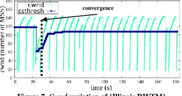
When using RWTM with Illinois, the player converges, as presented in Figure 7. The congestion rate is very low (CNG=0.55), but congestions are caused by the aggressiveness of Illinois (the concave curve of cwnd in the C-AIMD approach) and its high ssthresh value (120 MSS). Congestions slow down the convergence speed and slightly reduce the QoE due to the multiplicative decrease approach of Illinois. As shown in Figure 7, one congestion event delayed the convergence time to 27 seconds. In addition, Illinois has the ability to select the suitable ssthresh value (110 MSS in Figure 7) that minimizes congestion events in the future, in spite of the sensitivity of RWTM to congestions. OFF* periods still exist, but with low frequency (frOFF* = 0.22).

Figure 7. Cwnd variation of {Illinois RWTM},

IS=2.40%, IF=5.47%, V=27s, frOFF*=0.22, CNG=0.55

The Cubic variant yielded good performances with both shaping methods. The variations of cwnd when Cubic is combined with HTBM and RWTM are presented in Figures 8 and 9, respectively.

In Figure 8, the player converges tardily after a delay of 33 seconds. The cause is mainly the low value of ssthresh that is selected by the Cubic algorithm. As explained in Subsect. 2.1, the HyStart algorithm, implemented in Cubic, defines

convergence

12 this ssthresh in order to have a less aggressive increase of

cwnd. The ssthresh becomes lower when the RTTC-S

increases. Knowing that HTBM increases RTTC-S by

introducing an additional queuing delay, HyStart decreases

ssthresh to be approximately 57 MSS. This is why the

player cannot upgrade to its optimal quality level n° 4 before convergence. The second cause is the multiplicative decrease approach of Cubic and the high rate of congestions caused by HTBM. This second cause makes the convergence to optimal quality level more difficult because the server is not able to increase its reduced congestion window cwnd during the ON period, as it should be increased.

After convergence, many congestions were recorded, and

OFF* periods were negligible. The ssthresh becomes more

stable around 75 MSS: this is well-set by the HyStart algorithm. This enhances stability in the congestion avoidance phase with a more uniform increase of cwnd, as shown between 60 and 80 seconds in Figure 8. Furthermore, there is a set of large cubic curves with inflection points close to the ssthresh value. The variable

cwnd is more present in the convex region, which is more

aggressive when moving away from the inflection point.

Figure 8. Cwnd variation of {Cubic HTBM},

IS=1.98%, IF=19.03%, V=33s, frOFF*=0.16, CNG=186.11 In Figure 9, the player converges rapidly in only 8 seconds. The ssthresh begins with a low value (60 MSS) for a few seconds during the buffering state, and then the HyStart algorithm implemented in Cubic rapidly adjusts the ssthresh value and enables the server to be more aggressive. Comparing with Figure 7, selecting a lower initial value of

ssthresh is better for accelerating convergence, because

otherwise there are more risks of congestion that slow down the convergence speed.

Congestions are infrequent: only two congestions are visible in Figure 9 at seconds 70 and 130, and they are resolved by fast retransmission in accordance with Algorithm 1 and by using Hystart. As a consequence, separated congestion events do not dramatically affect the performance, as when Illinois is used with RWTM (Figure 9). The Cubic algorithm chooses the inflection point to be around 140 MSS, which is much higher than the ssthresh value, so that the concave region becomes more aggressive

than the convex region. The OFF* periods persist, even with Cubic, but with a low frequency: frOFF* = 0.22.

Figure 9. Cwnd variation of {Cubic RWTM}, IS=1.78%,

IF=5.5%, V=8s, frOFF*=0.22, CNG=1.66

Accordingly, the Cubic variant is able to adjust its congestion window curve in different situations. When many congestions occur, the cubic curve becomes rather convex to carefully increase cwnd. When many OFF* periods occur, the cubic curve becomes rather concave, and is thus more aggressive than the concave curve of Illinois in order to rapidly achieve the desired send bitrate and compensate for the reduction of the cwnd value. However, Cubic begins by estimating a low value of ssthresh that is adjusted over time by the HyStart algorithm, which is beneficial only when using RWTM as a shaping method. Using HTBM slows down convergence considerably and affects the infidelity metric.

4.2 Scenarios 2 and 3

In this section, we present the five performance measurements of client 1 for the first three scenarios described in Subsect. 3.2. We make the assumption that the optimal quality level of client 1 is n° 4. We do not present NewReno and Vegas variants because they demonstrated low performance. The average values of QoE metrics for client 1 in the first three scenarios are listed in Table 5, and the average values of CNG and frOFF* in the first three

scenarios are listed in Table 6. Both tables show the total mean values (denoted by MV) over the three scenarios. MVs are the global performance values proposed for consideration to compare between different combinations.

Table 5. QoE for client 1 in scenarios 1, 2, and 3

T CP var ian t S ce n a ri o Performance metric

Instability (%) Infidelity (%) Convergence speed (seconds) HTBM RWTM HTBM RWTM HTBM RWTM Cub ic 1 1.86 1.63 20.45 5.02 52.06 19.55 2 3.44 1.43 32.90 3.42 64.13 10.98 3 2.19 1.63 18.49 4.81 34.65 14.34 MV* _{2.49 1.56 23.95 4.42 50.28 14.96} Ill in ois 1 1.56 1.88 7.75 6.17 21.10 24.22 2 3.20 1.56 29.75 4.42 59.58 13.28 3 1.85 1.76 7.92 5.66 21.03 18.80 MV 2.20 1.73 15.14 5.42 33.90 18.56 convergence convergence