Validation of a simplified analysis for the simulation of delamination of CFRP composite laminated materials under pure mode I

HAL Id: hal-02467697

https://hal.archives-ouvertes.fr/hal-02467697

Submitted on 5 Feb 2020

HAL is a multi-disciplinary open access

archive for the deposit and dissemination of

sci-entific research documents, whether they are

pub-lished or not. The documents may come from

teaching and research institutions in France or

abroad, or from public or private research centers.

L’archive ouverte pluridisciplinaire HAL, est

destinée au dépôt et à la diffusion de documents

scientifiques de niveau recherche, publiés ou non,

émanant des établissements d’enseignement et de

recherche français ou étrangers, des laboratoires

publics ou privés.

Validation of a simplified analysis for the simulation of

delamination of CFRP composite laminated materials

under pure mode I

Frederic Lachaud, Eric Paroissien, Laurent Michel

To cite this version:

Frederic Lachaud, Eric Paroissien, Laurent Michel. Validation of a simplified analysis for the

simula-tion of delaminasimula-tion of CFRP composite laminated materials under pure mode I. Composite

Struc-tures, Elsevier, 2020, 237, pp.1-19. �10.1016/j.compstruct.2020.111897�. �hal-02467697�

an author's

https://oatao.univ-toulouse.fr/25266

https://doi.org/10.1016/j.compstruct.2020.111897

Lachaud, Frédéric and Paroissien, Eric and Michel, Laurent Validation of a simplified analysis for the simulation of

delamination of CFRP composite laminated materials under pure mode I. (2020) Composite Structures, 237. 1-19.

ISSN 0263-8223

Validation of a simplified analysis for the simulation of delamination of

CFRP composite laminated materials under pure mode I

Frédéric Lachaud

_{, Eric Paroissien, Laurent Michel}

Institut Clément Ader (ICA), Université de Toulouse, ISAE-SUPAERO, INSA, IMT MINES ALBI, UTIII, CNRS, 3 Rue Caroline Aigle, 31400 Toulouse, France

Keywords:

Delamination

Thermoset composite material Macro-element

Cohesive zone model DCB

4 points L-shape bending

A B S T R A C T

The cohesive zone modelling (CZM) is extensively used for the simulation of delamination propagation of composite laminated materials. The Finite Element (FE) method is able to support the CZM. Nevertheless, a refined mesh in the cohesive zone is required to describe accurately the energy dissipation. A 1D-beam simplified analysis based on the macro-element (ME) technique has been developed for the stress analysis of bonded joints, supporting damage evolution adhesive material law. The objective of this paper is to provide a validation of the ability of this macro-element technique for the simulation of delamination propagation in pure mode I of composite laminates. This validation is led through a comparative study between experimental test results, 3D FE model predictions and 1D-beam ME predictions. The experimental test campaign allows in particular for the assessment of the interlaminar strength and critical energy release rate in pure mode I. The thermoset uni-directional (UD) prepreg composite material IMA/M21E is used for this paper.

1. Introduction

The composite laminated materials exhibit excellent mechanical in-plane strengths, the direction of which can be oriented along a wanted direction. Moreover, the strength-to-mass ratio is so attractive, that industrial sectors, for which the mass of high strength structures is a stake, such as aerospace or automotive, exhibit the highest interest in the composite laminated materials. For example, the recent airliners A350 XWB and B787 Dreamline content at least 50% of composite la-minated materials in weight [1]. However, the strength of structures made of composite laminated materials can be reduced by delamination

[2]. In order to experimentally assess the strength of composite lami-nated materials against delamination, it is common to use precracked test specimens, such as double cantilever beam (DCB) or end notch flexure (ENF) test specimens. The delamination process takes then place along the selected interface from the precrack location, allowing for the measurement of critical energy release rates related to mode loading at crack tip. Cohesive zone modelling (CZM) eventually in conjunction with Finite Element (FE) is commonly used to simulate the delamina-tion process[3–9]. Nevertheless, a refined mesh has to be employed to accurately represent for the high stress gradient at crack tip and then for the energy dissipation[10–13]. That is why the reduction of com-putational time receives the attention of several research teams

[12,14–18]. The authors of the present papers and co-workers have

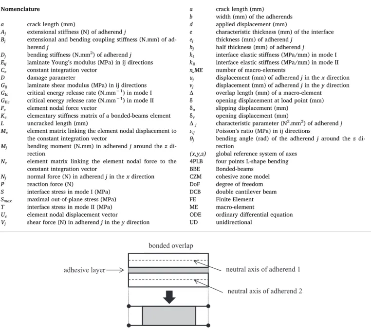
been working on the development of the macro-element (ME) tech-nique for the simplified stress analysis of bonded, bolted and hybrid (bonded/bolted) joints[19–21]. In particular, the elementary stiffness matrix of a dedicated 4-node Bonded-Beams (BBe), has been formulated for the modelling of bonded overlap (seeFig. 1). The 4 nodes rely on the neutral axes of each adherend, which can be dissimilar and modelled as Euler-Bernoulli or Timoshenko laminated beams. Like the cohesive zone modelling (CZM), the adhesive layer is modelled as a bed of shear and peel springs, representing for the link between both adherend in-terfaces. The formulation of the elementary stiffness matrix consists in determining the linear relationships between the nodal forces and the nodal displacements (see Fig. 2). Once the stiffness matrix of the complete structure is assembled from the elementary matrices and the boundary conditions are applied, the minimization of the potential energy provides the distributions of displacements, internal forces, stresses and strains in both the adherends and the adhesive layer. The ME technique is inspired by the FE method and differs in the sense that the interpolation functions are not assumed. Indeed, they take the shape of solutions of the governing ordinary differential equations (ODEs) system, coming from the constitutive equations of the adhesive and adherends and from the local equilibrium equations, related to the simplifying hypotheses. The direct consequence is that only one ME is needed to predict the distribution of displacements, internal forces, stresses and strains in both the adherends and the adhesive layer at

https://doi.org/10.1016/j.compstruct.2020.111897

⁎_{Corresponding author.}

every location of the structure, in the frame of a linear elastic analysis. In the case of a nonlinear analysis, a mesh along the overlap is required. Nevertheless, contrary to classical FE model, it is not necessary to mesh in the thickness, so that a benefit in terms of computational time is obtained.

The objective of this paper is to provide a validation of the ability of the simplified analysis, based on the macro-element technique, initially developed for the stress analysis of adhesively bonded joints, for the simulation of delamination propagation in pure mode I of composite laminates. This simplified analysis shall reduce the number of degrees of freedom (DoFs) required to describe the delamination propagation while ensuring accurate predictions. For the comfort of readers, this paper provides in a first part the useful mathematical steps describing the simplified analysis, although they are already presented in[19–21]

for the simulation of debonding of bonded joints. It is indicated that this approach is not able to capture the variation of the delamination front along the width with or without eventual elastic coupling, since the approach presented is developed in the 1D-beam framework. The reader is referred to[22]for this topic. An experimental test campaign

is then presented on the thermoset unidirectional (UD) prepreg com-posite material IMA/M21E. The experimental test campaign aims at assessing the interlaminar mechanical behavior in pure mode I, in order to determine the parameters associated to the traction-separation law of the CZM, which are the maximal interlaminar out-of-plane tensile stress, the critical energy release rate and the interface stiffness. It is indicated that this work does not discuss about the shape choice of the traction-separation law. The reader can refer to other published works about this topic (eg:[23–25]). The four points L-shape bending (4PLB) test allows for the assessment of the maximal interlaminar out-of-plane tensile stress, while the DCB test according to ASTM Standard D5528-01[26]is used for the critical energy release rate. The interface stiff-ness is chosen of the order of magnitude 1.105_MPa.mm−1_[10]and

adjusted to correlate the experimental test results on DCB specimens. The validation of the ME technique for the simulation of delamination propagation in pure mode I is led on the precracked DCB test specimens against the predictions of 3D FE models and experimental test results. The numerical test campaigns are then presented in the fourth part of this paper, including the assessment the performance of the simplified

Nomenclature

a crack length (mm)

Aj extensional stiffness (N) of adherend j

Bj extensional and bending coupling stiffness (N.mm) of

ad-herend j

Dj bending stiffness (N.mm2) of adherend j

Eij laminate Young’s modulus (MPa) in ij directions

Ce constant integration vector

D damage parameter

Gij laminate shear modulus (MPa) in ij directions

GIc critical energy release rate (N.mm−1) in mode I GIIc critical energy release rate (N.mm−1) in mode II

Fe element nodal force vector

Ke elementary stiffness matrix of a bonded-beams element

L uncracked length (mm)

Me element matrix linking the element nodal displacement to

the constant integration vector

Mj bending moment (N.mm) in adherend j around the z

di-rection

Ne element matrix linking the element nodal force to the

constant integration vector

Nj normal force (N) in adherend j in the x direction

P reaction force (N)

S interface stress in mode I (MPa)

Smax maximal out-of-plane stress (MPa)

T interface stress in mode II (MPa)

Ue element nodal displacement vector

Vj shear force (N) in adherend j in the y direction

a crack length (mm)

b width (mm) of the adherends

d applied displacement (mm)

e characteristic thickness (mm) of the interface

ej thickness (mm) of adherend j

hj half thickness (mm) of adherend j

kI interface elastic stiffness (MPa/mm) in mode I kII interface elastic stiffness (MPa/mm) in mode II

n_ME number of macro-elements

uj displacement (mm) of adherend j in the x direction

vj displacement (mm) of adherend j in the y direction

Δ overlap length (mm) of a macro-element

δ opening displacement at load point (mm)

δu slipping displacement (mm)

δv opening displacement (mm)

Δj characteristic parameter (N2.mm2) of adherend j

ν_ij Poisson’s ratio (MPa) in ij directions

θj bending angle (rad) of the adherend j around the z

di-rection

(x,y,z) global reference system of axes

4PLB four points L-shape bending

BBE Bonded-beams

CZM cohesive zone model

DoF degree of freedom

DCB double cantilever beam

FE Finite Element

ME macro-element

ODE ordinary differential equation

UD unidirectional

analysis through a comparative study. The MATLAB code for the si-mulation of DCB test leading to the results presented in this paper is provided as supplementary materials.

2. Description of the simplified analysis

2.1. Analysis framework 2.1.1. Idealization

A pre-cracked laminated specimen is considered. Its length is L + a, where a is related to the crack length. As a result, the pre-cracked la-minated specimen is seen as two laminates which are bonded only over an interface along the uncrack length L. Each laminate within the cracked region is then modelled as a beam element, while both the laminates and the interface within the uncracked region are modelled by one 4-nodes ME (seeFig. 2). In the case of nonlinear computation, a mesh of n_ME MEs is employed along the uncracked length. The pre-cracked laminated specimen is then idealized as a structure under 1D-beam kinematics involving n_ME + 2 elements, 2n_ME + 4 nodes and then 6n_ME + 12 degrees of freedom (DoF).

2.1.2. Hypotheses

In order to formulate the stiffness matrix of beam elements and MEs, the following hypotheses are taken: (i) the laminates are simulated by linear elastic Euler-Bernoulli laminated beams and (iii) the interface is simulated by an infinite number of elastic shear and transverse springs.

2.1.3. Governing equations

The constitutive equations can be written as (seeAppendix A):

= = N A du dx B d dx, j 1, 2 j j j j j ₍₁₎ = + = M Bdu dx D d dx, j 1, 2 j j j j j ₍₂₎ =dv = dx j 1, 2 j j ₍₃₎

where Njis the normal force in the adherend j, Vjthe shear force in the

adherend j, Mj the bending moment in the adherend j, uj the

long-itudinal displacement in the adherend j, vj the deflection in the

ad-herend j θj the bending angle in the adherend j, Ajis the membrane

stiffness of adherend j, Bjthe coupling membrane-bending stiffness of

adherend j and Djthe bending stiffness of adherend j. In the case of a

lay-up characterized by a mirror symmetry, Bj= 0. The subscript j = 1

(j = 2) refers to the upper (lower) laminate.

The constitutive equations for the interface are provided by:

= = S k vI[ 1 v2] kI v (4) = + = T k uII[ 2 h2 2 (u1 h1 1)] kII u (5) with: = v v v 1 2 (6) = u u h h u 2 1 2 2 1 1 (7)

where kI (kII) the interface stiffness in mode I (II). δu (δv) is

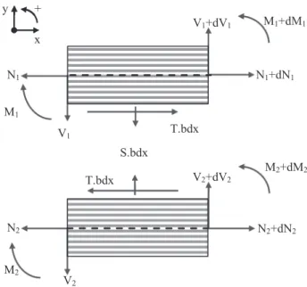
re-presentative of the slipping (opening) displacement of the interface. The local equilibrium of each laminate provides the following equations (seeFig. 3):

= = dN dx ( 1)bT j, 1, 2 j _j (8) = + = dV dx ( 1) bS j, 1, 2 j _{j 1} (9) + + = = dM dx V bh T 0,j 1, 2 j j j ₍₁₀₎ with: = = h e j 2, 1, 2 j j ₍₁₁₎

where ejis the thickness of the adherend j.

2.2. Formulation of elementary stiffness matrix

The elementary stiffness matrix of a beam element is provided in

Appendix C. The elementary stiffness matrix of ME is representative for the linear relationship between the vector of nodal forces Feand the

vector of nodal displacements Ue(seeFig. 4), such as: = = F K U N N N N V V V V M M M M K u u u u v v v v (0) (0) ( ) ( ) (0) (0) ( ) ( ) (0) (0) ( ) ( ) (0) (0) ( ) ( ) (0) (0) ( ) ( ) (0) (0) ( ) ( ) e e e e 1 2 1 2 1 2 1 2 1 2 1 2 1 2 1 2 1 2 1 2 1 2 1 2 (12)

where Keis the elementary stiffness matrix of the ME and Δ is the length

of the ME.

In order to determine the components of Ke from the governing

equations, the approach consists in expressing (i) the adherend dis-placements as a function of the abscissa, (ii) the adherend internal force using the constitutive equations (Eqs. (1–3)), (iii) the nodal displace-ments and normal forces as function of a set of integration constants, such as:

=

Ue M Ce e (13)

=

Fe N Ce e (14)

where Ce is the vector of the integration constants, Me the matrix

linking the displacement nodal vector Ueand Ce, and Ne the matrix

linking the nodal force vector Feand Ce. The elementary stiffness matrix

Ke is then obtained by a matrix product:

= = =

Fe N Ce e N M Ue e 1 e Ke N Me e 1 (15)

The adherend constitutive equations Eqs. (1–2) are written such as:

= + = du dx D N BM j, 1, 2 j j j j j j j (16) = + = d dx B N AM j, 1, 2 j j j j j j j (17) where Δj= AjDj-BjBj≠ 0.

By combining equations Eqs. (4–5), (8–10) and (16–17), the fol-lowing system of ODEs in terms of interface stresses is obtained:

= + d T dx k dT dx k S 3 3 1 2 ₍₁₈₎ = d S dx k dT dx k S 4 4 3 4 (19) where: = + + + + k bk D 1 h A D h A h B h B D 1 D 2 1 II 1 1 12 1 1 2 2 22 2 2 1 1 1 2 2 2 (20) = + + k2 bkII h A1 1 h A B B 1 2 2 2 1 1 2 2 (21) = + + k3 bkI h A1 1 h A B B 1 2 2 2 1 1 2 2 (22) = + k4 bkI A1 A 1 2 2 (23)

The system of ODEs in Eqs. (18–19) can be uncoupled by differ-entiation and linear combination as:

+ + = d S dx k d S dx k d S dx (k k k k S) 0 6 6 1 4 4 4 2 2 2 3 1 4 ₍₂₄₎ + + = d dx d T dx k d T dx k d T dx (k k k k T) 0 6 6 1 4 4 4 2 2 2 3 1 4 ₍₂₅₎

This system is solved and the adhesive shear and peel stresses are thus written as (seeAppendix C):

= + + + + +

S x

K e tx K e tx K e tx K e tx K e K e

( )

sin cos sin cos

sx sx sx sx rx rx

1 2 3 4 5 6

(26)

Fig. 3. Free body diagram of infinitesimal pieces included between x and

x + dx of both adherends in the overlap region. Subscript 1 (2) refers to the

upper (lower) adherend.

= + + + + + +

T x K e tx K e tx K e tx K e tx K e K

e K

( ) sxsin sxcos sxsin sxcos rx

rx

1 2 3 4 5 6

7 (27)

There are then 13 integration constants. However, by introducing these previous expressions for adhesive stresses in equation Eqs. (18–19), the integration constants of the adhesive peel stress appear to be linked to those of adhesive shear stress as:

= K K K K K K K K K K K K 0 0 0 0 0 0 0 0 0 0 0 0 0 0 0 0 0 0 0 0 0 0 0 0 0 0 1 2 3 4 5 6 1 2 2 1 1 2 2 1 3 3 1 2 3 4 5 6 (28) where: = s s t k k ( 3 ) 1 2 2 1 1 (29) =t t s +k k ( 3 ) 2 2 2 1 2 (30) =r r k k ( ) 3 2 1 2 (31)

It comes then seven independent integration constants remain: K1to K7.

Following the resolution scheme in[27,28], the displacements and internal forces in the adherends are expressed as functions of adhesive stresses and of their derivatives. The computation is fully detailed in

Appendix D. It is shown that a total number of twelve integration constants are finally involved: K1to K7, J1to J3and J5to J6. The

dis-placements in the adherends are then expressed as:

= + + + u x T dS dx b K B J A x J x J ( ) 6 2 1 1 1 3 7 1 0 1 2 5 6 (32) = + + + + + + + + + u x T dS dx b K B J A x J h hJ x J h hJ h h K ( ) 6 2 2 ( ) 2 2 2 3 7 2 0 2 2 5 1 2 1 6 1 2 2 1 5 1 6 7 ₍₃₃₎ = + + + + + + v x k dT dx k d S dx S J x _J x _J x _J ( ) 1 3 4 2 2 2 5 0 3 1 2 2 3 (34) = + + + + + + v x k dT dx k d S dx S J x _J x _J x _J ( ) 2 4 4 2 2 2 6 0 3 1 2 2 3 (35) = + + + + x T dS dx J x _J x _{J K} ( ) 3 2 1 1 5 5 0 2 1 2 5 7 ₍₃₆₎ = + + + + x T dS dx J x _J x _{J K} ( ) 3 2 1 2 6 6 0 2 1 2 6 7 ₍₃₇₎

The nodal displacements are then the values of displacements in

x = 0 and x = Δ, leading to Me. The adherend constitutive equations in

Eqs. (1–2) allow for the computation of normal and shear forces and of

bending moments in both adherends:

= + + + N x a dT dx a d S dx bK x B J AJ J ( ) 2 1 1 1 2 2 7 1 2 1 1 5 6 ₍₃₈₎ = + + + + + N x a dT dx a d S dx bK x h h A B _J A_J ( ) 2 ( ) 2 2 2 2 2 7 1 2 2 2 2 1 2 5 (39) = + V x a d T dx a d S dx bh T J b K A ( ) 6 B 1 3 2 2 3 3 3 1 1 0 3 1 7 1 3 (40) = + V x a d T dx a d S dx bh T J b K A ( ) 6 B 2 4 2 2 4 3 3 2 2 0 3 2 7 2 3 (41) = + + + + M x a dT dx a d S dx J b K A x D J B J ( ) 6 B 2 1 3 3 2 2 1 0 3 1 7 1 2 1 2 1 1 5 ₍₄₂₎ Table 1

Mechanical parameters of the UD laminate IMA/M21E.

E11(MPa) E22= E33

(MPa) G(MPa)12= G13 G23(MPa) ν(MPa)12= ν13 ν23(MPa)

= + + + + + M x a dT dx a d S dx J b K A x D h h B J B J ( ) 6 B 2 ( ) 2 4 4 2 2 2 0 3 2 7 2 2 2 1 2 2 2 1 25 ₍₄₃₎

The nodal forces are then assessed in x = 0 and x = Δ, leading to

Ne. The stiffness matrix of the pre-cracked specimen can then be built

from the elementary stiffness matrices using the classical FE rules.

3. Experimental testing

3.1. Materials

The thermoset unidirectional (UD) prepreg composite material IMA/M21E is used in this paper. The ply thickness is 0.133 mm. The mechanical parameters of this laminate are provided in Table 1, re-sulting from a classical test campaign which is not presented in this paper.

3.2. Manufacturing of test specimens

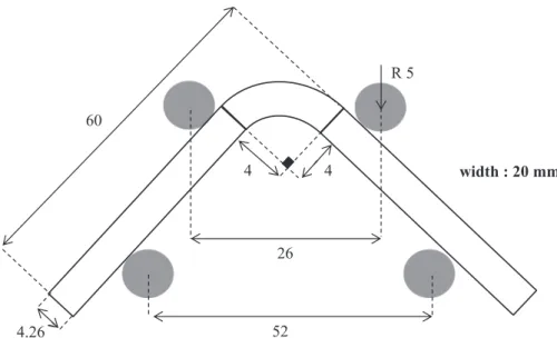
Two types of specimens have to be manufactured: 4PLB specimens (strength test) and DCB specimens (propagation test). The lay-up is performed by hand with prepeg cut thanks to a specific jig. It provides laminated plates for the DCB specimens. A dedicated apparatus is used to form the L-shape specimens (seeFig. 5).

For the 4PLB test specimens, the stacking lay-up is [0]32. For the

DCB test specimens, the stacking lay-up is [0]20. In order to create the

pre-crack length of propagation test specimens, a Teflon® film (0.013 mm thickness) is applied between both relevant plies. The manufacturing of these plates is realized using an autoclave under a curing temperature of 180 °C and a pressure of 7 bars, during two hours, such as compliant with the supplier recommendations. The specimens are then cut from the cure plate with a diamant tool at the final dimensions (seeFigs. 6and7).

3.3. Experimental set-up

All the tests are performed on an INSTRON tensile machine, the capacity of the load cell of which is 10,000 N and 200 N for 4PLB and

Fig. 6. 4PLB test specimen. Dimensions in mm (principle scheme, not to scale).

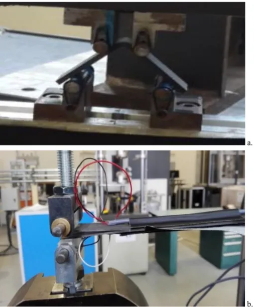
Fig. 8. Installation of specimens to be tested: a) 4PLB specimen, b) DCB specimen.

DCB tests, respectively. The loading is applied at controlled crosshead displacement at a rate equal to 0.5 mm.min−1_{and 5 mm.min}−1_for

4PLB, and DCB tests, respectively. The reaction force and the total displacement are measured by the tensile machine. For the 4PLB test specimen, a full field displacement measurement VIC 3D (Digital Image Correlation System) is introduced and placed in front of each sample; experimentally a random pattern with good contrast is applied to the through thickness surface of specimens. A calibration process, per-formed before loadings, allows for the establishment of the accurate position of both cameras. Displacement, load, strain sensors and 3D field measurement, were recorded simultaneously with a 10 Hz (1 Hz for 3D camera) frequency rate and stored. For the DBC tests, the length of the actual crack is measured using a Fractomat® gauge. In order to remove the accumulation of matrix at the crack tip due to the presence of Teflon® film, a first loading run is realized to propagate delamination

[29]. The initial pre-cracked length is then not anymore equal to 45 mm but to the measured one. The installation of specimens to be tested is

illustrated inFig. 8.

3.4. Experimental test results 3.4.1. 4PLB tests

A total number of 5 specimens are tested. The reaction force as a function of the total displacement δ of the two rolls is shown inFig. 9. The objective of this tests is to determine the out plane failure stresses

Smaxof the ply interface. As a result, only the force at failure for the first

delamination propagation is kept. The average value recorded is 532 N with a standard deviation equal to 17 N.

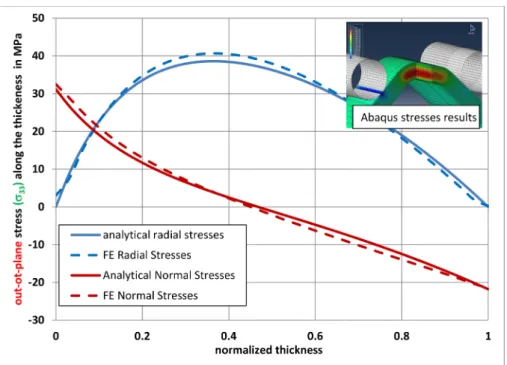
These results are used to compute the out-of-plane stress in two ways: the first one by an analytical solution given by Ko[30,31]using composite laminates applied to curved beam; the second one by a FE numerical model [32]developed on ABAQUS® software. The reader will be able to read the references given for more details about these models. For each model, a critical average force is imposed and the

Fig. 10. 4PLB tests: out-of-plane stresses and in-plane stresses in fibers direction along thickness in the middle of the L-shape beam.

Fig. 11. DCB experimental test result: reaction force as a function of the opening displacement at load point for a = 45 mm (see the web version in which each curve

resulting out-of-plane stresses are plotted inFig. 10as a function of the height. The value of the maximal out-of-plane stress considered for the CZM is then Smax= 40 MPa.

3.4.2. DCB tests

A total number of 5 specimens are tested. The reaction force as a function of the opening displacement at load point, termed δ, is pro-vided inFig. 11. The data reduction is performed following the mod-ified beam theory[26], allowing for the assessment of the critical en-ergy release rate in mode I:

= + G P b a 3 2 ( ) c L I (44) where P is the force, b is the width of the specimen and ΔLthe lag in

crack length at a zero value of compliance. The force peaks vary from 33 N to 40 N. The average value is equal to 36.5 N with a standard deviation equal to 2.63 N. The stiffnesses before the peak force are very close. The behavior during the propagation of the delamination shows parallel curves indicating similar values the critical energy release rate between each test.

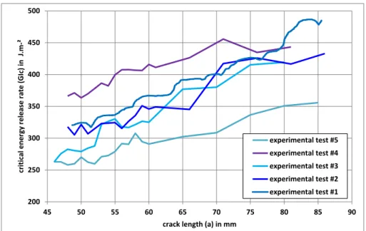
A R-curve effect is classically observed (seeFig. 12), due to fiber bridging between both arms during the propagation. In other words, the value for GIc varies with the crack length. Over the range of crack

propagation, the average value for GIc is included between

0.306 N.mm−1_{and 0.404 N.mm}−1_{. The average of these average}

va-lues is 0.368 N.mm−1 _{with a standard deviation equal to}

0.044 N.mm−1_{. For the simulation work presented in this paper, it is}

considered that the value of GIcis constant. The value of the critical

energy release rate considered for the CZM is then GIc= 0.4 N.mm−1.

4. Numerical testing

4.1. Geometry and material modelling

The geometrical models used for the propagation test specimen are based on the geometry of experimental test specimens (Fig. 13). The geometrical parameters are given inTable 2. The classical laminate theory[33]is employed to compute the homogenized stiffness of la-minated arms, used in the numerical tests. The interface between both arms is represented through a CZM based on a classical bilinear traction separation law. The maximal stress, the initial stiffnesses and the cri-tical energy release rate in pure mode I are required to define the bi-linear traction separation law in mode I (Table 4). The maximal stresses are taken from the strength experimental tests while the critical energy release rates from the propagation experimental tests. The initial stiff-ness is adjusted to fit the experimental force displacement curves (Fig. 10). Besides, the definition of the traction separation law in mode II is provided inTable 4. Even if the DCB test leads to a pure mode I, the interface stiffness in pure II is at least required as an input data. The results presented come from a test campaign on the pure mode II, which is not presented here, based on interlaminar shear strength test[34]

and end-notched flexure test[35]. Based on the provided geometrical

Fig. 12. Critical energy release rate as function of the crack length.

Fig. 13. Geometry conditions for the DCB test specimen simulated (principle scheme, not to scale). The downwards and upwards arrow indicate the location of load

application.

Table 2

Geometrical parameters for the DCB test specimen.

a (mm) b (mm) e1= e2(MPa) L (mm)

and material configurations, the numerical models presented in this paper are of two types: (i) 3D FE model and (ii) 1D-beam ME model, presented inSection 4.2andSection 4.3respectively. The 3D FE model is developed using the FE code ABAQUS General Standard software. The laminates in the 3D FE model are modelled with the ply orthotropic properties provided inTable 1. In the 1D-beam ME model, the homo-genous properties provided in Table 4 and deduced from the ply properties are used. The interface stiffness in mode I is determined to fit at best the initial stiffness of the experimental test results on DCB specimen (Section 3.4.2). A value of 85,000 MPa.mm−1_{is found, which}

has the same order of magnitude found in[10]for example.

4.2. 3D FE modelling 4.2.1. Boundary conditions

The loading applied to the DCB specimens is relevant to the ex-perimental test set-up. The DCB specimens are loaded under controlled displacement along the thickness direction (y-axis ofFig. 13). For the DCB specimen, the loading is applied thanks to reference points linked to the nodes of arms through rigid body elements to represent for the tabs. The rotation around the width direction (z-axis ofFig. 13) of re-ference points is free. Finally, contact conditions are introduced be-tween all the surfaces in contact – the arms along the pcracked re-gion – are added, including classical Coulomb friction effect with a friction coefficient equal to 0.15.

4.2.2. Computation

The computation uses the Full Newton Raphson solver (ABAQUS General Standard) with nonlinear geometric activation. The full Newton Raphson scheme involved an update of the tangent stiffness matrix at each iteration; this scheme appears to the authors as a suitable approach to support the progressive failure of laminates. Moreover, the classical viscous regularization is activated with the related couple of parameters τ = 1E-4 s (viscous characteristic time) and a = 1 (damping parameter) [4,36]. It allows in particular for a better convergence within implicit scheme. Viscosity for element control option is disabled.

4.2.3. Mesh and convergence study

The laminates are meshed with quadratic brick elements under normal integration scheme: eight Gauss point and three DoF per nodes. Three elements in the thickness are used for each laminate. Each spe-cimen is shared in three distinct regions: (i) the pre-cracked region, (ii) the propagation regions and (iii) the remaining specimen region. The length of the propagation region is adjusted through successive tests to ensure that the remaining specimen region is not damaged at the maximal applied load. To ensure a correct representation for the bending, the pre-cracked and the remaining specimen regions have a mesh density according to the length direction (x-axis ofFig. 13) and

the width direction is one element per mm. Within the propagation region, the mesh is refined such that the mesh densities are two ele-ments per mm according to the length direction and one element ac-cording to the width direction. To simulate the delamination propa-gation between the laminates, cohesive elements are used. The cohesive elements are linked to the laminates through a non-coincident kine-matic bonding. It allows for the performing of a convergence study at lower computational time, since the mesh of the cohesive element is independent on the mesh of laminates. The mesh density according to width direction is the same as the laminates while the mesh density according to the length direction, which is the propagation direction, varies between two and sixteen cohesive element per mm. A view of the mesh and loading conditions is provided inFig. 14.

The results of the convergence study are presented for the DCB specimen. The reaction force as function of the opening applied dis-placement (δ = 2d) and of the applied disdis-placement (d) are provided in

Fig. 15for the DCB specimen. Five mesh densities are selected: one, two, four, eight and sixteen elements per mm. From four elements per mm, the convergence in terms of critical energy release rate is achieved. Nevertheless, oscillations remain significant at a density of four ele-ments per mm, due to local instability of the element failure associated with too elevated element length. From eight elements per mm, the oscillations appear as negligible, so that this mesh density is considered as sufficient. Finally, the shape of the delamination crack is classically found as curved[29].

4.3. 1D-beam ME modelling 4.3.1. Modelling using ME

The use of CZM for the simulation of delamination of composite materials implies a nonlinear computation to predict the current da-mage state. Even if a detailed description of the nonlinear algorithm used is provided in[20], a brief overview is provided hereafter for the comfort of the reader. Once the stiffness matrix of the pre-cracked specimen is built using a uniformly distributed mesh (Section 2), the boundary conditions have to be applied. They are defined in terms of fixed displacements and assigned displacements d = 5 mm for the DCB specimen (Fig. 16). The Augmented Lagrangian method[37,38]is then used allowing for the simultaneous assessment of both displacements and reactions. A Newton-Raphson algorithm based on the secant matrix is employed. The assigned displacements are applied linearly as func-tion of the numerical time through a uniformly distributed time step-ping involving fifty time steps. The secant matrix is updated at each iteration within each time step to reach the equilibrium under a con-vergence threshold equal to 1.10-3_{on the nodal force vector. The secant}

matrix update consists in updating the interface stiffnesses kIand kII.

For illustration purpose, the pure mode I is considered. In the case of the bilinear damage evolution law, a damage parameter is computed

Fig. 15. a) Reaction force as function of the applied opening displacement for the five mesh densities for the DCB specimen. A focus around the maximal applied force

is provided. b) process zone and crack front shape for 8 FEs/mm and d = 10 mm (SDEG is the damage parameter D).

only if δv > 0 through: = D ( ) ( ) v f v v e v v v f , , , (45)

where δ v,e(δ v,f) is the displacement jump at damage initiation

(propagation). A damage parameter is computed at each pair of nodes. As each ME has two pairs of nodes, each ME has two damage meters associated. It is then chosen to assign a unique damage para-meter D to each ME equal to the maximal value of damage parapara-meters computed at each of both pairs of nodes. Moreover, if the damage parameter computed is strictly higher than a prescribed value then it is fixed to this value, which is chosen equal to 0.9999999 in this paper. The secant matrix is then updated through the update of the interface stiffness in mode I: kIbecomes (1−D)kI. The material and geometrical

parameters given inTables 2–4are used.

4.3.2. Convergence study

A convergence study is undertaken to justify a correct energy

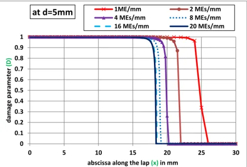
dissipation[10,13]. The selected mesh densities along the interface are 1 ME per mm, 2 MEs per mm, 4 MEs per mm, 8 MEs per mm, 16 MEs per mm and 20 MEs per mm. The reaction force as function of the opening applied displacement (δ = 2d) and of the applied displacement (d) for the six mesh densities are provided inFig. 17for the DCB spe-cimen. It is shown then that the numerical simulations tend to a steady global behavior for a mesh density higher than 16 MEs per mm. Besides, it is then shown that the computational methodology described in this paper leads to a convergence of numerical predictions in terms of cri-tical energy released rates. When the density of MEs is too low, the energy dissipated is lower than the critical energy release rates. In terms of local behavior, the same conclusion holds, as shown by the dis-tribution of the damage parameter along the overlap at the maximal applied displacement inFig. 18for the DCB specimen.

4.4. Comparison

The experimental test results as well as the numerical test results provided 1D-beam ME and 3D FE models are plotted inFig. 19in terms of reaction force as a function of the opening displacement at the load point. From a macroscopic point of view, both numerical models are in good agreement with the experimental test results. The numerical test results show a correct energy released rate during propagation. The discrepancy between the predictions an experimental test results are due to the choice of a constant value GIc. As shown inSection 3.4.2, the

value of GIcvaries during the propagation (R-curve effect). Relatively to

Table 3

CZM parameters in pure mode I and pure mode II.

stress

displacement

jump

mode I

k

G

S

stress

displacement

jump

mode II

G

k

T

kI(N.mm−1) Smax(MPa) GIc(N.mm−1) kII(N.mm−1) Tmax(MPa) GIIc(N.mm−1)

85,000 40 0.4 75,000 85 0.7

Table 4

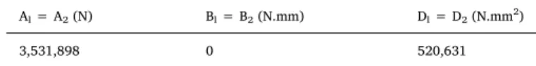
Homogenized stiffness of arm based on 10 plies of IMA/M21E (eply= 0.133 mm).

Al= A2(N) Bl= B2(N.mm) Dl= D2(N.mm2)

3,531,898 0 520,631

the 3D FE model, the 1D-beam ME model appears to have a slightly higher initial stiffness and a lesser maximal (−3.77%). The difference in initial stiffness is due to the modelling of the laminated. In the 1D-beam ME model, it is a pure isotropic transverse laminate with a ply per ply approach whereas in the 3D FE model it is a homogeneous ortho-tropic laminate. As a consequence, the process of damage initiation and propagation appears earlier in the 1D-beam ME model than in the 3D FE model, leading to a difference in maximal force. Besides, it is in-teresting to compare the local response of both models. The length of the process zone is then a judicious indicator. It corresponds to the length where the damage parameter is strictly higher than 0 and lower than 1. For example, under an opening displacement at load point

δ = 10 mm, the process zone is then measured equal to 1.3125 mm for

the 3D FE model and to 6.75 mm for the 1D-beam ME model. It is then highlighted that the local mechanical behavior is dependent on com-putation strategy fort the damage parameter. In the 3D FE model, the damage parameter is computed at each Gauss point, modified by the

viscous regularization of the cohesive law and bounded at a maximal damage value of 0.999. In the 1D-beam ME model, the damage para-meter is computed as the maximum of damage parapara-meter obtained at both pairs of nodes of each ME and bounded by a maximal damage value of 0.9999999 (see Section 4.3.1). The predicted process zone appears as dependent on the computation strategy in plus to be related to the cohesive law of the interface. The question is then to develop an experimental methodology to assess the cohesive law shape as well as the process zone, representative for the physics.

5. Conclusions

In this paper, the validation of the ability of a simplified analysis, based on the ME technique, for the simulation of delamination propa-gation in pure mode I of composite laminates is presented. The vali-dation is based on the comparison of experimental test results, 3D FE predictions and 1D-beam ME predictions on pre-cracked DCB test

Fig. 18. Damage parameter distribution along the interface (up to 30 mm from the crack tip) at the maximal applied displacement (d = 5 mm) for the six mesh

densities for the DCB specimen.

specimens. The interface CZM in pure mode I is priory assessed in terms of maximal cohesive stresses and critical energy release rates through dedicated experiments on 4PLB and DCB test specimens. The interface stiffness is adjusted through the 3D FE models. The thermoset UD prepreg composite material IMA/M21E is used in this paper. When using the CZM interface assessed as an input, it is shown that the 1D-beam ME predictions of the global mechanical behavior are in close agreement with the 3D FE predictions and experimental test results. Compared to a classical 3D FE model with CZM, a first interest of the ME technique of the simulation of the delamination propagation is the reduction of the number of DoF, while refining the mesh along the interface to be delaminated. It is due to the fact that the specimen is only meshed along its length (and not along its width and thickness). Indeed, the displacement field are not assumed but have the shape of the solutions of the governing ODEs system (Section 2andAppendix C). The ME stiffness matrix is then easily evaluated through a matrix pro-duct from the expressions for the nodal displacements and nodal forces (Appendix E). As a result, a computational time reduction could be expected. Moreover, a second interest of the ME technique is the re-lative simplicity of implementation and use. It is then a relevant ap-proach for the pre-sizing, optimization process and analysis of labora-tory tests, involving various loadings (including temperature variation), boundary conditions or material and geometrical parameters. A last interest is that the ME technique takes advantage from its compatibility with the FE method. The ME could be implemented in FE codes. Methodologies developed for the improvement of numerical perfor-mance of CZM based on FE models could be applied to the ME tech-nique, when relevant. In[20], the ME technique has been successfully applied for the simulation of the debonding of adhesive bonded joints under pure mode I, pure mode II and mixed-mode I/II loadings. Due to

the results presented in this paper for the simulation of delamination of propagation under pure mode I, it could be thought that the ME tech-nique is suitable for the simulation of delamination of propagation under pure mode II and mixed-mode I/II too. Finally, even if both models provide similar predictions in terms of global mechanical be-haviours, those in terms of local behaviours are dependent on the computation strategy for a same cohesive law of the interface. It means that the local physics could not be correctly retrieved, so that the choice of the cohesive law associated with the computation strategy is ques-tionable[24].

CRediT authorship contribution statement

Frédéric Lachaud: Conceptualization, Methodology, Validation,

Formal analysis, Investigation, Writing - original draft, Writing - review & editing. Eric Paroissien: Conceptualization, Methodology, Software, Validation, Formal analysis, Investigation, Writing - original draft, Writing - review & editing. Laurent Michel: Methodology, Validation, Formal analysis, Investigation.

Declaration of Competing Interest

The authors declare that they have no known competing financial interests or personal relationships that could have appeared to influ-ence the work reported in this paper.

Acknowledgement

This work has not received any specific grant.

Appendix A

This appendix provides the derivation of the constitutive equations of laminated beams used in the 1D-beam analysis, in the (X,Yi,Z) reference

local axis of the adherend, the height origin of which is taken on the neutral axis. The normal force and the bending moment are written such as:

= + = = = N Xi( ) _h bdY b dY i, 1, 2 h i i p n h h ip i 1 i i i i pi pi _i 1 _(A.1) = + = = = M Xi( ) _h Y bdY b Y dY i, 1, 2 h i i i p n h h ip i i 1 i i i i pi pi _i 1 _(A.2)

where, in the adherend i niis the number of layers and hpiis the final height of the pithlayer.

Moreover, the orthotopic behavior provides

=Q ,i=1, 2

ipi ipiipi (A.3)

where, in the adherend i, Qipiis the matrix of reduced stiffness in the p_ithlayer.

As a result, the normal force and the bending moment are given by:

= = = N Xi( ) b Q dY i, 1, 2 p n h h ip ip i 1 i i pi pi _{i i} 1 _(A.4) = = = M Xi( ) b Q Y dY i 1, 2 p n h h ip ip i i 1 i i pi pi _{i i} 1 _(A.5)

which finally leads to:

= = = N X Q dY du dX b Q Y dY d dX ( ) i p n ip h h i i p n ip h h i i i 1 1 i i i pi pi i i i pi pi 1 1 _(A.6) = + = = M X b Q Y dY du dX b Q Y dY d dX ( ) i p n ip h h i i i p n ip h h i i i 1 1 2 i i i pi pi i i i pi pi 1 1 _(A.7)

The parameters involving in the constitutive equations Eqs. (1)–(3) are thus defined such as for i = 1,2:

= = Ai b Q (h h ) p n ip p p 1 1 i i i i i (A.8)

= = B b Q h h 2 ( ) i p n ip p p 1 2 12 i i i i i (A.9) = = D b Q h h 3 ( ) i p n ip p p 1 3 13 i i i i i (A.10) Appendix B

The elementary stiffness matrix Kjfor the beam j (j = 1,2), the length of which is a, can be derived following the approach describes inSection 2

such as: = + +

(

) (

)

(

) (

)

This appendix describes the resolution of the differential equation system in Eqs. (24–25). The characteristic polynomial expression is:

= + + = P R( ) R3 k R k R (k k k k) 0 1 2 4 2 3 1 4 (C.1) where: = R r2 _(C.2)

To determine the roots, the Cardan’s method is employed. Then, equation (C.1) is modified as:

+ + = R'3 p R' q 0 _(C.3) where: = R' R k 3 1 (C.4) = + p k k 3 12 4 _(C.5) = + q k k k k k k k 27(2 9 ) 1 12 4 2 3 1 4 _(C.6)

The determinant is:

=q + 4p 27 2 3 (C.8) By defining: = q + u 2 3 (C.9) = q v 2 3 (C.10) the roots of the reduced equation are written as:

= + R₁' u v _(C.11) = + R uei ve i 2' 2 3 23 (C.12) = + R uei ve i 3' 4 3 43 (C.13)

Consequently, the roots of the characteristic equation (C.1) are given by:

= + + = R u v k r

3

= + + = + R 1 i s it 2(u v) 3 2 (u v) ( ) 2 2 _(C.15) = + = R 1 i s it 2(u v) 3 2 (u v) ( ) 3 2 _(C.16)

Finally, the expressions for the interface stresses are given in Eqs. (26–27) where:

= + + r u v k 3 1 (C.17) = + s 1 Re R R 2( ( )2 | |)2 (C.18) = t 1 Re R R 2( ( )2 | |)2 (C.19)

Re(z) stands for the real part and |z| for the modulus of z.

Appendix D

This appendix describes the determination of expressions for the adherend displacements and internal forces. Using the constitutive equations of adherends in Eqs. (1–3) and the local equilibrium equations in Eqs. (8–10) it is possible to express the derivatives of the longitudinal and transverse displacements as functions of the adhesive stresses and their derivatives:

= + d v dx A dT dx B S 4 1 4 10 10 _(D.1) = + d v dx A dT dx B S 4 2 4 20 20 (D.2) = + d u dx C dT dx D S 3 1 3 10 10 (D.3) = + d u dx C dT dx D S 3 2 3 20 20 _(D.4) where: = + A10 b (B h A ) 1 1 1 1 (D.5) = B10 bA1 1 (D.6) = A20 b (B h A ) 2 2 2 2 (D.7) = B20 bA2 2 (D.8) = + C10 b (h B D ) 1 1 1 1 (D.9) = D10 bB1 1 (D.10) = + C20 b( h B D ) 2 2 2 2 (D.11) = D20 bB2 2 (D.12)

To obtain the expressions for displacements in the adherends, Eqs. (D.1-D.4) have to be integrated. Before integrating equations Eqs. (D.1-D.4), the system of ODEs in Eqs. (18–19) are written as:

= + S d T dx d S dx 1 k k2 3 k k1 4 k3 k 3 3 1 4 4 _(D.13) = + dT dx d T dx d S dx 1 k k1 4 k k2 3 k4 k 3 3 2 4 4 _(D.14)

and introduced in Eqs. (D.1–D.4). The displacements in the adherends are then expressed as:

= + + + + u C D T C D dS dx J x _J x _J k k k k k k k k k k k k 1 10 4 10 3 1 4 2 3 10 2 10 1 1 4 2 3 4 2 5 6 (D.15)

= + + + + u C D T C D dS dx J x J x J k k k k k k k k k k k k 2 20 4 20 3 1 4 2 3 20 2 20 1 1 4 2 3 4 2 5 6 (D.16) = + + + + + + v A B dT dx d S dx A B _{S J} x _J x _J x _J k k (k k k k ) k k k k k k k k 1 10 4 10 3 1 4 2 32 4 2 2 2 10 2 10 1 1 4 2 3 0 3 1 2 2 3 (D.17) = + + + + + + v A B dT dx d S dx A B _{S J} x _J x _J x _J k k (k k k k ) k k k k k k k k 2 20 4 20 3 1 4 2 32 4 2 2 2 20 2 20 1 1 4 2 3 0 3 1 2 2 3 (D.18) =A B T K + A B dS + + + dx J x _J x _J k k k k k k ( ) k k k k k k 3 2 1 1 10 4 10 3 1 4 2 3 7 10 2 10 1 1 4 2 3 0 2 3 1 2 2 _(D.19) = A B T K + A B dS + + + dx J x J x J k k k k k k ( ) k k k k k k 3 2 1 2 20 4 20 3 1 4 2 3 7 20 2 20 1 1 4 2 3 0 2 3 1 2 2 _(D.20)

Fourteen new integration constants are involved. However, following the resolution scheme in[27,28], the total number of integration constants can be reduced to twelve. Firstly, the local equilibrium equation along the x-axis for the adherend 2 (Eq. (1) with j = 2) in conjunction with the constitutive equation in normal force (Eq. (8) with j = 2) gives:

= = dN bdx T A d u dx B d v dx bT 2 2 2 2 2 2 3 2 3 (D.21) leading to: = = + A J B J bK J b K A B J A 2 6 2 3 2 ₂4 2 ₃0 7 4 2 7 2 2 0 2 (D.22)

In the same way, by considering the adherend 1, it comes:

= + J b K A B J A 2 3 4 2 7 1 1 0 1 (D.23)

Secondly, the difference between the deflections of both adherends provides:

= + + + + v v S k J J x J J x J J x J J ( ) ( ) ( ) 1 2 I 0 0 3 1 1 2 2 2 3 3 (D.24) But, considering the constitutive equation of the interface in mode I (Eq. (4)), it comes:

= = Ji J ii, 1, 2, 3 (D.25) Since: + + = D D h B h B k kII 10 20 1 10 2 20 2 _(D.26) = C C h A h BA k k 20 10 1 10 2 20 1 II (D.27)

the difference in the longitudinal displacements of the interface provides:

= +

u u h h T

k P x( )

2 1 2 2 1 1

II (D.28)

where P(x) is a quadratic polynomial, all coefficients of which have to be equal to zero:

= J4 J4 3h1J0 3h2J0 0 _(D.29) = J5 J5 2h1J1 2h2J1 0 _(D.30) + + + = J J hJ h J K k h A h A k h AB h B k k k k [ ( ) ( )] 0 6 6 1 2 2 2 7 1 4 2 3 4 1 10 2 20 3 1 10 2 20 (D.31)

It is then deduced that the integration constant set J1, J2, J3, J5and J6is independent. The displacements take then the shape in Eqs. (32–37) with

the following parameters:

= C k D k k k k k 1 10 4 10 3 1 4 2 3 (D.32) =C k D k k k k k 1 10 2 10 1 1 4 2 3 (D.33) =C k D k k k k k 2 20 4 20 3 1 4 2 3 (D.34)

=C k D k k k k k 2 20 2 20 1 1 4 2 3 (D.35) =A k B k k k k k 5 10 4 10 3 1 4 2 3 (D.36) = A k B k k k k k 5 10 2 10 1 1 4 2 3 (D.37) =A k B k k k k k 6 20 4 20 3 1 4 2 3 (D.38) = A k B k k k k k 6 20 2 20 1 1 4 2 3 (D.39) = k k k k 3 5 1 4 2 3 (D.40) = k k k k 4 6 1 4 2 3 (D.41) = + + +

(

)

(

)

The constitutive equations of adherends in Eqs. (1–3) allow for the computation of normal and shear forces and of bending moments in both adherends such as provided in Eqs. (38–43) as with the following parameters:

= a1 A1 1 B1 5 (D.43) = a1 A1 1 B1 5 (D.44) = a2 A2 2 B2 6 (D.45) = a2 A2 2 B2 6 (D.46) = + a3 B1 1 D1 5 (D.47) = + a3 B1 1 D1 5 (D.48) = + a4 B2 2 D2 6 (D.49) = + a4 B2 2 D2 6 (D.50) References

[1] Marsh G. Composites consolidate in commercial aviation. Reinf Plast 2016;60(5):302–5.

[2] Riccio A. Delamination in the context of composite structural design. In: Sridharan S, editor. Woodhead publishing series in composites science and engineering, de-lamination behaviour of composites. Cambridge, England: Woodhead Publishing Limited; 2008. p. 28–64.

[3] Allix O, Ladevéze P. Interlaminar interface modelling for the prediction of dela-mination. Compos Struct 1992;22:235–42.

[4] Allix O, Ladevéze P, Corigliano A. Damage analysis of interlaminar fracture speci-mens. Compos Struct 1995;31:61–74.

[5] Chaboche J, Girard R, Schaff A. Numerical analysis of composite systems by using interphase/interface models. Comput Mech 1997;20(1–2):3–11.

[6] Alfano G, Crisfield MA. Finite element interface models for the delamination ana-lysis of laminated composites: mechanical and computational issues. Int J Numer Meth Engng 2001;50:1701–36.

[7] Camanho PP, Davila CG, Ambur DR, 2001. Numerical simulation of delamination growth in composite materials. NASA/TP-2001-211041, Hampton, VA. [8] Goyal VK, Johnson ER, Dávila CG, Jaunky N. Irreversible constitutive law for

modeling the delamination process using interfacial surface discontinuities. Compos Struct 2004;65:289–305.

[9] Wisnom MR. Modelling dsicrete failures in composites with interfaces elements. Compos Pt A 2010;41:795–805.

[10] Turon A, Dávila CG, Camanho PP, Costa J. An engineering solution for mesh size effects in the simulation of delamination using cohesive zones models. Eng Fract Mech 2007;74:1665–82.

[11] Harper PW, Hallet SR. Cohesive zone length in numerical simualtions of composite delamination. Eng Fract Mech 2008;75:4774–92.

[12] Alvarez D, Blackman BRK, Guild FJ, Kinloch AJ. Mode I fracture in adhesively-bonded joints: a mesh-size independent modelling approach using cohesive ele-ments. Eng Fract Mech 2014;115:73–95.

[13] Martin E, Vandellos T, Leguillon D, Carrère N. Initiation of edge debonding: coupled criterion versus cohesive zone model. Int J Fract 2016;199:157–68.

[14] Guiamatsia I, Davies GAO, Ankersen JK, Iannucci L. A framework for cohesive element enrichment. Compos Struct 2010;92(2):454–9.

[15] Yang QD, Fang XJ, Shi JX, Lua J. An improved cohesive element for shell delami-nation analyses. Int J Numer Meth Engng 2010;83(5):611–41.

[16] Do BC, Liu W, Yang QD, Su XY. Improved cohesive stress integration schemes for cohesive zone elements. Eng Fract Mech 2013;107:14–28.

[17] Ersoy N, AhmadvashAghbash M, Engül M, Öz FE. A comparative numerical study aiming to reduce computation cost for mode-I delamination costs. Proceedings of 18th european conference on composite materials (ECCM 2018), 25–28 June 2018, Athens (GR). 2018.

[18] Russo R, Chen B. High order adaptively integrated cohesive element. Proceedings of 18th european conference on composite materials (ECCM 2018), 25–28 June 2018, Athens (GR). 2018.

[19] Paroissien E, Sartor M, Huet J, Lachaud F. Analytical two-dimensional model of a hybrid (bolted/bonded) single-lap joint. J Aircraft 2007;44:573–82.

[20] Lélias G, Paroissien E, Lachaud F, Morlier J, Schwartz S, Gavoille C. An extended semi-analytical formulation for fast and reliable mode I/II stress analysis of adhe-sively bonded joints. Int J Solids Struct 2015;62:18–38.

[21] Lélias G, Paroissien E, Lachaud F, Morlier J. Experimental characterization of co-hesive zone models for thin adco-hesive layers loaded in mode I, mode II, and mixed-mode I/II by the use of a direct method. Int J Solids Struct 2019;158:90–115. [22] Rzeczkowski J, Samborski S, Valvo PS. Effect of stiffness matrices terms on

dela-mination front shape in laminates with elastic couplings. Struct Comput 2019.

https://doi.org/10.1016/j.compstruct.2019.111547. in press.

cohesive-zone models. Compos Sci Technol 2006;66:723–30.

[24] Jaillon A, Jumel J, Paroissien E, Lachaud F. Mode I cohesive zone model parameters identification and comparison of measurement techniques for robustness to the law shape evaluation. J Adhesion 2019.https://doi.org/10.1080/00218464.2019. 1669450.

[25] Skec L. Identification of parameters of a bi-linear cohesive-zone model using ana-lytical solutions for mode-I delamination. Eng Fract Mech 2019;214:558–77. [26] Standard Test Method for Mode I Interlaminar Fracture Toughness of Unidirectional

Fiber-Reinforced Polymer Matrix Composites, 2001. ASTM.

[27] Högberg JL. Mechanical behavior of single-layer adhesive joints – an integrated approach Licensing Graduate Thesis Sweden: Department of Applied Mechanics, Chalmers University of Technology; 2004

[28] Alfredsson KS, Högberg JL. A closed-form solution to statically indeterminate ad-hesive joint problems-exemplified on ELS-specimens. Int J Adhes Adhes 2008;28(7):350–61.

[29] Prombut P, Michel L, Lachaud F, Barrau JJ. Delamination of multidirectional composite laminates at 0°/Theta° ply interfaces. Eng Fract Mech

2006;7(16):2427–42.

[30] Ko WL, 1988. Delamination stresses in semicircular laminated composite bars. NASA TM 4026.

[31] Ko WL, Jackson RH, 1989. Multilayer theory for delamination analysis of a

composite curved bar subjected to end forces and end moments. NASA TM 4139. [32] Michel L, Garcia S, Yao C, Espinosa C, Lachaud F, 2014. Experimental and

nu-merical investigation of delamination in curved beam multidirectional laminated composite specimen. Key Engineering Materials Vols. 577-578 (2014) pp 389-392, Advances in Fracture and Damage Mechanics XII, Trans Tech Publications, Switzerland, doi:10.4028/www.scientific.net/KEM.577-578.389.

[33] Reddy JN. Mechanics of laminated composite plates and shells: theory and analysis. 2nd ed., CRC Press; 2004. ISBN 0-8493-1592-1.

[34] Standard Test Method for Short-Beam Strength of Polymer Matrix Composite Materials and Their Laminates, 2016. ASTM.

[35] Standard Test Method for Determination of the Mode II Interlaminar Fracture Toughness of Unidirectional Fiber-Reinforced Polymer Matrix Composites, 2014. ASTM.

[36] Sola C, Castanié B, Michel L, Lachaud F, Delabie A, Mermoz E. On the role of kinking in the bearing failure of composite laminates. Compos Struct 2016;141:184–93.

[37] Curnier A, Alart P. A generalized Newton method for contact problems with fric-tion. J Theor Appl Mech 1988;7(1):67–82.

[38] Simo JC, Laursen TA. An augmented lagrangian treatment of contact problems involving friction. Comput Struct 1992;42(1):97–116.