Long-Range Road Detection for Off-line Scene
Analysis
Jean-Philippe Tarel
LCPC (LEPSIS), 58 Boulevard Lef`ebvre, 75015 Paris, France
Email: [email protected]
Erwan Bigorgne
Majority-report, 15 rue clavel,75019 Paris, France
Email: [email protected]
Abstract—Long-range detection of road surface in a sequence
of images from a front camera aboard a vehicle is known as an unsolved problem. We propose an algorithm using a single camera and based on color segmentation which has interesting performance and which is stable along the sequence whatever its length. It is an off-line algorithm which makes good use of current and successive images to build reliable models of the color aspects of the road and of its environment at each vehicle position. To apply the proposed algorithm a radiometric calibration step is required to ensure uniform responses of the pixels over the image. The algorithm consists in three steps: image smoothing consistent with perspective effect on the road, building of the models of the road and non-road colors, and region growing of the road region. The relevance of the proposed algorithm is illustrated by an application to the roadway visibility estimation in stereovision and its performance are illustrated by experiments in difficult situations.
I. INTRODUCTION
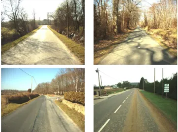
Studies on road surface detection started in the early days of automatic road-following applications for which the first step was a segmentation of the road surface from images acquired with a camera mounted on a vehicle. Different algorithms to discriminate between road and non-road regions were proposed using a gray-level or a color camera [1], [2], [3], [4], [5]. However, as noticed by most of these authors, the segmentation of the road surface faces many difficulties which can be grouped in two categories: the spatial and temporal variabilities of the color aspect of the road and of its environment. The temporal variability can be due for instance to seasons, shadows moving with sun position, sky color (blue, cloudy, sunset), changes in illumination between successive pictures due to clouds, weather conditions such as fog, or specular reflection when the sun is low on the horizon. Examples of spatial variability are the presence of dirt on the road, change of asphalt type, and asphalt patches due to road fixing. Examples of these perturbations are shown in Fig. 1. As a consequence, in the past two decades, research in road-following mainly focussed on marked roads. Nevertheless road surface detection was improved in two directions:
• search for features more discriminative than the RGB colors such as texture [6], depth in stereovision [7], color space robust to shadows [8], [9],
• and model based approaches using the road shape geom-etry [10], [11], [12], [13].
Fig. 1. Examples of difficult images for road surface detection.
Despite these improvements, the road surface detection and segmentation problem is still only partially solved especially at long distances.
For single intelligent vehicle applications, the fact that long-range detection of road surface cannot be solved is not always a limitation. Indeed, many applications such as road-following or free space detection only require the detection at a limited range ahead of the vehicle. However, intelligent vehicles can also be used to diagnose the road and its environment, this information being saved for future use by the same vehicle or shared through a communication network for use by other vehicles. In this context, long-range road detection is of main importance for the knowledge of the road: it allows 3D road profile estimation and reconstruction [14]. Then, collected data on the shape of the road can be used in many applications such as roadway visibility distance assessment [15], image contrast restoration in presence of fog [16], [17], long-range obstacle detection [18]. The key point when dealing with diagnostic from intelligent vehicles is to observe that it does not require real time. Therefore, the processing can make use of the images before and after the current vehicle position. This implies important new possibilities of processing in particular towards reliable and accurate long-range detection of road surface.
(a) (b)
Fig. 2. Regions for road and non-road colors sampling on each image (a) and equivalent road regions for a sequence (b).
This paper is structured as follows: in Sec. II, we present how to model the road colors off-line for stable processing, and then we describe the proposed algorithm for long-range detection of road surface in Sec. III. The road surface detection algorithm being sensitive to lens vignetting, we propose in Sec. IV a simple technique for automatic radiometric calibra-tion that does not require any controlled acquisicalibra-tion. Then in Sec. V, an application to roadway visibility distance estimation is described. Finally in Sec. VI, we present experiments that assess the performance of the proposed detection algorithm and we discuss its limits.
II. STABLECOLORMODELS
The difficulty of long-range detection of road surface is due to the extrapolation of road colors from small to large distances. Extrapolation is known to perform poorly when the function to extrapolate is subject to large variations, as it is the case for the road colors as a function of the distance. Off-line processing allows us to reformulate the problem as an interpolation where the road colors are sampled on the current image It and also in the successive images It+1, It+2,· · · Usually, the colors of the road are sampled using a window located at the bottom center of each image, assuming that the vehicle is driving on the road not too close to any other vehicle, like the green trapezoid in Fig. 2(a). At a given image, by sampling road colors in the bottom center of several of its successive images, we sample road colors along the vehicle path and thus at increasing distances to the current vehicle position. This sampling in successive images is similar to sampling road colors along the road seen in the current image, as shown in Fig. 2(b). A decay factor is applied recursively from one image to another. It induces that road colors sampled in too far images are exponentially forgotten.
This idea was already used in [15] by processing the image sequence backward for road colors but not for non-road colors. In that approach, the non-road color model, used to process It, is based on the colors of the pixels not classified as
road in It+1. This yields to an error accumulations along the sequence and thus a not enough stable behavior of the detection algorithm. For a stabler algorithm, we propose a very cautious sampling of the non-road colors in the current and successive images: non-road colors are sampled into two relatively small triangles at the top of every image, see Fig. 2(a). The top center region is not considered since it
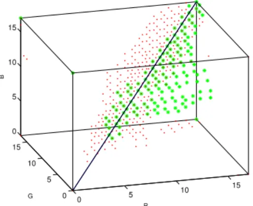
0 5 10 15 0 5 10 15 0 5 10 15 R G B
Fig. 3. Road (green stars) and non-road (red points) colors in the RGB space.
may contain a gray colored sky region which is a source of difficulties. For similar reasons, the road colors are sampled in a reduced region in the bottom center of the image, where we are sure that road pixels only will be observed whatever the road geometry.
To be fully generic, we use a non-parametric model, i.e the road and non-road colors are modeled as probability distribu-tions over the RGB color space. In practice, the RGB color space is discretized in18 × 18 × 18 bins, and the road (or non-road) probability distribution is represented as an histogram of road (or non-road) pixel colors. Fig. 3 displays non-zero bins of typical road and non-road RGB histograms. These distributions are far from Gaussian or mixture of Gaussian. This demonstrate the importance of using a non parametric model here. Due to the generality of this model, we obtained similar results using other color spaces with 3 degrees of freedom, assuming the number of bins is large enough.
III. ROADDETECTIONALGORITHM
The inputs of the long-range road detection algorithm are at each step: the image to be processed, a probability ratio threshold rth, a decay factor, and road and non-road color models. The former model is an histogram of the road colors sampled from the bottom centered region in the successive images (without using the current image). The latter model is an histogram of the non-road colors sampled from the top left and right regions in the successive images (again, without using the current image).
A. Pre-Smoothing
When observed by a front camera in the vehicle, the road is seen in a large range of distances, due to the perspective effect. In particular, while the road texture can be seen near the vehicle, the width of the road is only a few pixels at long distances. As a consequence, pixel samples extracted from the bottom center of the image mainly models the variations of the road texture colors, and do not describe well its aspect at far range. To circumvent this difficulty, a progressive image smoothing is needed. The role of this pre-processing is to
(a) (b)
(c) (d)
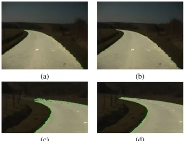
Fig. 4. Road segmentation results without (a) and with (b) smoothing. (c) and (d) are zooms at long distances of (a) and (b). The maximum standard deviation of the smoothing is only 11 pixels.
equalize or at least to reduce the scale range of the details seen on the road in the image. The width of the road decreases linearly with the image height until it reaches zero at the horizon. Therefore, the standard deviation of the smoothing function must also decrease linearly with the image height. For easier and faster processing, the average smoothing is 1D and applied along lines. Its standard deviation is 1 pixel for lines from the image top to the horizon line, then the standard deviation increases until it reaches its maximum at the bottom line of the image.
Fig. 4 shows comparative results obtained without and with this smoothing on a road with strong texture. It can be seen how the segmentation at long distances is noticeably improved by the smoothing.
B. Road Growing
After the smoothing, a decay factor is multiplied to the road and non-road color histograms obtained from the successive images. Then these class-conditional histograms are respec-tively updated by adding the samples of the bottom center and of the top left and right regions of the current image. The current probability distribution of the road colors is initialized using the road color histogram previously obtained.
The segmentation algorithm is a growing algorithm of the road region. The seed at the initialization of the growing is the bottom centered road region of Fig. 2(a). The criterion to include a pixel into the road region is:
• the pixel must have at least 3 of its 8 neighbors in the road region,
• and the pixel colors C must satisfy P(C|road) ≥ P(C|non − road) × rthwhere rthis the probability ratio threshold.
The neighborhood constrain is necessary to stop growing into very thin regions. The second constrain is the classical
Bayesian decision ratio for color classification between two classes: road and non-road. However, it is not written as a ratio in order to properly handle the case where P(C|road) and/or P(C|non − road) are zero.
Each time a pixel is included in the road region, the probability distribution of the road colors is updated by taking into account its color in the distribution. For consistency, we thus constrain the road region not to grow into the non-road and sky regions, see Fig. 2(a). This update helps to grow the road region into pixels with colors of low probability ratio by increasing its probability of being in the road. Due to the shape of the second constrain, it also allows to include colors not classified in road and non-road classes in the road class. This gives to the growing algorithm better generalization capabilities.
It is important to notice, that in the obtained segmentation, the pixels classified as road do not have the same detection confidence values. Indeed, a pixel with a large probability ratio has more chances to be correctly classified than one with a smaller probability ratio. Therefore, the ratio P(C|non−road)P(C|road) can be used as a detection confidence value for every road pixels in further processing steps.
IV. ROADRADIOMETRICCALIBRATION
In the previous segmentation algorithm, pixel responses are assumed uniform. This uniformity is usually not obtained in practice due to light fallout and lens vignetting. As shown in Fig. 5(a), the darker borders are the typical effect produced by lens vignetting. To restore the pixel responses uniformity, it is necessary to perform the so-called radiometric calibration. It exits several techniques for radiometric calibration, see [19] for a complete overview. Most of them implies the use of a calibration setup or needs several images of the same scene, and thus are not of pratical use in our context. Assuming that pixel responses are the same up to a linear factor which varies along the radius to the image center, we propose a simple and efficient technique dedicated to road images allowing to perform the radiometric calibration from a single image. Indeed, the road, as shown in Fig. 5(a) is generally present on a large region of the image. The road surface can be assumed to be mainly uniform when correctly chosen in a sequence, and therefore used as a calibration setup.
The road radiometric calibration consists in the following steps:
1) Select an image where the pavement seems to have an approximatively uniform color in the sequence of images.
2) Smooth the image as explained in previous section to cancel the texture of the road near the vehicle.
3) Keep the bottom half triangle of the image and remove all pixels with too white colors.
4) For every pixel of the previous region, compute the associated point (di, gi) where di the distance of the pixel to the image center and gi is its gray level value. 5) Perform a robust fit using Iterative Reweighted Least Squares (IRLS) [20] on the previous data points using
(a)
(b)
(c)
Fig. 5. The borders of the original image (a) are affected by light fallout. The road pixels are selected in the triangle and the points (pixel distance dito
the image center, pixel gray level gi) are fitted by a even parabola to model
the light fallout (b). After correction using the proposed road radiometric calibration (c), the fallout is mostly removed.
the linear model gi= a0+ a1d2
i (or by a higher degree even polynomial model), as shown in Fig. 5(b). Notice that the estimated fallout is assumed an even function of the distance, and thus the previous line fitting in d2i is equivalent to the fit an even parabola as a function of di.
6) Correct the intensity of every pixels of the original images by dividing with the factor1 +a1
a0d
2
i, where di is the distance of the pixel i to the image center. The result of the road radiometric calibration on the original image in Fig. 5(a) is shown in Fig. 5(c). The strong light fallout at the corners is corrected. The proposed technique can be also applied on the average of several images of the sequence for better accuracy (in such a case the second step can be removed). It is important to perform this radiometric calibration to avoid missing the road in image corners, and even more important to avoid the bias towards dark colors in the road color model. Fig 6 illustrates how this bias
(a) (b)
(c) (d)
Fig. 6. Comparison of obtained road detection without (a) and with (b) the road radiometric calibration. (c) and (d) are zooms at long distances of (a) and (b).
correction improves the obtained results at long distances. This demonstrates the importance of the radiometric calibration for growing the road region correctly at long distances.
V. ROADWAY VISIBILITY DISTANCE
The speed limit along a road is somehow related to the roadway visibility distance, i.e the maximum distance at which an obstacle on the road can be clearly seen by a driver. This visibility distance being geometric, its value at a certain position changes slowly due to vegetation growing, and sometimes due to new buildings or signs, not considering other vehicles. As a consequence, the roadway visibility distance is an interesting parameter to diagnose regularly for safety purpose. In particular it can be used to check the consistency of the speed limit signs with respect to the roadway visibility distance.
Using the road detection algorithm previously described, we design a process able to estimate this roadway visibility distance off-line from stereovision cameras mounted on a vehicle. The vehicle of the LRPC Strasbourg that we used is shown in Fig. 7(c). This vehicle acquires stereo images every 5 meters, for instance see Fig. 7(a) and (b). The road surface is detected in each image. These segmentations provide a mask on the original image edges allowing us to select only the edges on the road in the two images. Then, the two edge maps are aligned using [14] which results in an estimate of the vertical road profile. Fig. 7(d) shows the edges of the right image aligned with the left image. Notice how accurate the alignment is even at long distances, despite the fact that the road is in front of a hill.
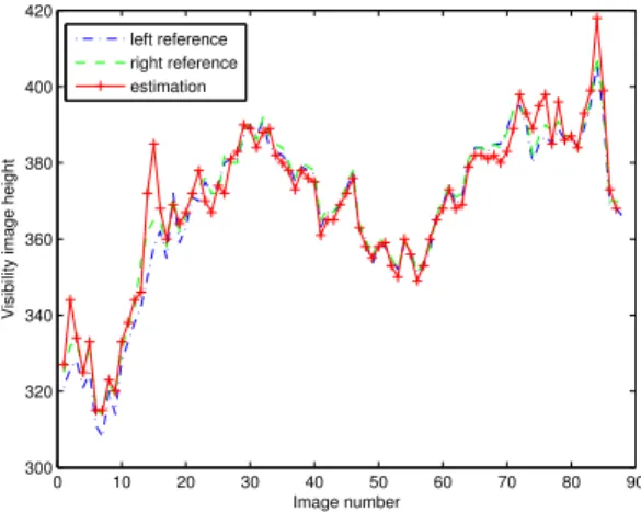
The image height of the roadway visibility is then defined as the maximum height at which the left and right edges match. It is displayed as an horizontal red line in Fig. 7(d). In Fig. 8, the estimated image height is compared with the ones obtained manually on the left and right images independently. In the sequence used, the vehicle is climbing a hill along a
(a) (b)
(c) (d)
Fig. 7. The estimated roadway visibility is shown as an horizontal red line in (d) and is obtained from the stereo images, after detection using the proposed algorithm, see (a) and (b). (c) is the vehicle used for the stereo acquisitions.
0 10 20 30 40 50 60 70 80 90 300 320 340 360 380 400 420 Image number
Visibility image height
left reference right reference estimation
Fig. 8. Comparison between the estimated image height of the roadway visibility and the ones manually obtained on the left and right images. A sequence of 90 images, when the vehicle is climbing a hill, is used.
450 meter long path (90 images). Finally, this image height of the roadway visibility can be retro-projected on the vertical road profile and the obtained value will be the estimate of the roadway visibility distance.
VI. EXPERIMENTS
To assess the performance of the proposed road surface detector, we built a database of 24 images with ground-truth. The 24 images were extracted from three different sequences taken in various countryside areas of France: near Nancy, Rouen and Saint-Brieuc. Each of these images was manually labeled with road and non-road labels. We use the classical evaluation by the Receiver Operating Characteristic (ROC) curve. The probability threshold rthis the decision parameter moved along the ROC curve. Fig 10 shows the large gain obtained using sampling in successive images compared to the
0 0.01 0.02 0.03 0.04 0.05 0.06 0.07 0 0.1 0.2 0.3 0.4 0.5 0.6 0.7 0.8 0.9 1
False positive rate
True positive rate
without with
Fig. 10. Comparison on 24 images database with ground-truth of the ROC curves with and without successive sampling along image sequence.
same algorithm with sampling only in the processed image. This demonstrates the importance of taking advantage of off-line processing when it is possible. This database with ground-truth is also used to better choose the parameters of the detection algorithm.
We applied the proposed road surface detection algorithm on different sequences covering paths from 2 to 10 kilometers long (each sequence comprises between 400 to 2000 images). We noticed a few situations where the road surface detector yields to over segmentations: specular reflection when the sun is near the horizon which can result in washed out colors, soil on the pavement the same colors as the fields on the road side, sunset which moves all the colors to orange, and clear gray buildings in urban environments. Nevertheless, in most of the other difficult situations, such as the ones shown in Fig. 1, we obtained successful results as shown in Fig. 9.
VII. CONCLUSION
We propose a reliable detection algorithm able to detect road surface from short to large distances in an image se-quence which does not suffer of divergences along time. This algorithm is off-line since it uses samples of the road and non-road colors in the current and subsequant images. The proposed algorithm is a growing segmentation with a dedicated pre-smoothing of the image and it is improved by the use of radiometric calibration. A simple and single image radiometric calibration algorithm is thus presented. The interest of off-line road surface detection is illustrated by a diagnostic application: the estimation of the roadway visibility distance, and experiments show the reliability of the proposed algorithms. Further improvements can be expected by extending the proposed algorithm to stereovision.
ACKNOWLEDGMENT
Thanks to Philippe Nicolle for building the reference im-ages, to LRPC Angers, Nancy and Strasbourg which provided us with the road images. Some of these images are property of DDE88 and the rest of LCPC. Thanks also to the Agence Nationale de la Recherche (ANR) for funding, within the ITOWNS-MDCO project.
Fig. 9. Road detection results on the difficult images of Fig. 1 and on other images. Detected road region is highlighted with a green border.
REFERENCES
[1] Matthew A. Turk, David G. Morgenthaler, Keith D. Gremban, and Martin Marra, “Vits-a vision system for autonomous land vehicle navigation,” IEEE Trans. Pattern Anal. Mach. Intell., vol. 10, no. 3, pp. 342–361, 1988.
[2] D. Kuan, G. Phipps, and A.-C. Hsueh, “Autonomous robotic vehicle road following,” IEEE Trans. Pattern Anal. Mach. Intell., vol. 10, no. 5, pp. 648–658, 1988.
[3] Charles Thorpe, Martial H. Hebert, Takeo Kanade, and Steven A. Shafer, “Vision and navigation for the carnegie-mellon navlab,” IEEE Trans.
Pattern Anal. Mach. Intell., vol. 10, no. 3, pp. 362–372, 1988.
[4] J.D. Crisman and C.E. Thorpe, “Unscarf, a color vision system for the detection of unstructured roads,” in Proceedings of the IEEE
International Conference on Robotics and Automation, Sacramento,
USA, 1991.
[5] S. Beucher, M. Bilodeau, and X. Yu, “Road segmentation by watersheds algorithms,” in Proceedings of the Pro-art vision group Prometheus
workshop, Sophia-Antipolis, France, April 1990.
[6] J. Zhang and H.-H. Nagel, “Texture-based segmentation of road images,” in Proceedings of the IEEE Intelligent Vehicles Symposium, 1994, pp. 260 – 265.
[7] K. Onoguch, N. Takeda, and M. Watanabe, “Planar projection stereopsis method for road extraction,” IEICE Transactions on Information
Systems, vol. E82-D, no. 9, pp. 10061018, 1998.
[8] P. Charbonnier, P. Nicolle, Y. Guillard, and J. Charrier, “Road bound-aries detection using color saturation,” in Proceedings of European
Signal Processing Conference (EUSIPCO’98), Rhodes, Greece, 1998,
pp. 2553–2556.
[9] R. Aufrere, V. Marion, J. Laneurit, C. Lewandowski, J. Morillon, and R. Chapuis, “Road sides recognition in non-structured environments by vision,” in Proceedings of the IEEE Intelligent Vehicles Symposium, Parma, Italy, 2004, pp. 329 – 334.
[10] S. Richter and D. Wetzel, “A robust and stable road model,” in
Proceedings of the 12th IAPR International Conference on Pattern
Recognition (ICPR’94), 1994, vol. 1, pp. 777–780.
[11] Miguel Angel Sotelo, Francisco Javier Rodriguez, Luis Magdalena, Luis Miguel Bergasa, and Luciano Boquete, “A color vision-based lane tracking system for autonomous driving on unmarked roads,” Auton.
Robots, vol. 16, no. 1, pp. 95–116, 2004.
[12] Yinghua He, Hong Wang, and Bo Zhang, “Color-based road detection in urban traffic scenes,” IEEE Transactions on Intelligent Transportation
Systems, vol. 5, no. 4, pp. 309–318, December 2004.
[13] O. Ramstrom and H. Christensen, “A method for following unmarked roads,” in Proceedings of the IEEE Intelligent Vehicles Symposium, 2005, pp. 650 – 655.
[14] J.-P. Tarel, S.-S. Ieng, and P. Charbonnier, “Accurate and robust image alignment for road profile reconstruction,” in Proceedings of the IEEE
International Conference on Image Processing (ICIP’07), San Antonio,
Texas, USA, 2007, vol. V, pp. 365–368, http://perso.lcpc.fr/tarel.jean-philippe/publis/icip07.html.
[15] E. Bigorgne and J.-P. Tarel, “Backward segmentation and region fitting for geometrical visibility range estimation,” in Proceedings of the Asian
Conference on Computer Vision (ACCV’07), Tokyo, Japan, 2007, vol. II,
pp. 817–826, http://perso.lcpc.fr/tarel.jean-philippe/publis/accv07.html. [16] N. Hauti`ere, R. Labayrade, C. Boussard, J.-P. Tarel, and D. Aubert,
“Perception through scattering media for autonomous vehicles,” in
Autonomous Robots Research Advances, Weihua Yang, Ed., chapter 8,
pp. 223–267. Nova Science Publishers, Inc., Hauppauge, NY, April 2008, http://perso.lcpc.fr/tarel.jean-philippe/publis/nova08.html. [17] N. Hauti`ere, J.-P. Tarel, and D. Aubert, “Towards fog-free in-vehicle
vision systems through contrast restoration,” in IEEE International
Con-ference on Computer Vision and Pattern Recognition (CVPR’07),
Min-neapolis, Minnesota, USA, 2007, pp. 1–8, http://perso.lcpc.fr/tarel.jean-philippe/publis/cvpr07.html.
[18] R. Labayrade, D. Aubert, and J.-P. Tarel, “Real time obstacle de-tection in stereo vision on non-flat road geometry through v-disparity representation,” in IEEE Intelligent Vehicle Symposium (IV’2002), Ver-sailles, France, 2002, vol. 2, pp. 646–651, http://perso.lcpc.fr/tarel.jean-philippe/publis/iv02.html.
[19] Seon Joo Kim and Marc Pollefeys, “Robust radiometric calibration and vignetting correction,” IEEE Transactions on Pattern Analysis and
Machine Intelligence (PAMI), vol. 30, no. 4, pp. 562–576, April 2008.
[20] S.-S. Ieng, J.-P. Tarel, and P. Charbonnier, “Modeling non-Gaussian noise for robust image analysis,” in Proceedings of International
Conference on Computer Vision Theory and Applications (VISAPP’07),
Barcelona, Spain, 2007, pp. 175–182, http://perso.lcpc.fr/tarel.jean-philippe/publis/visapp07a.html.