Virtual vibration measurement using KLT motion tracking algorithm

(1)

O

pen

A

rchive

T

oulouse

A

rchive

O

uverte (

OATAO

)

OATAO is an open access repository that collects the work of Toulouse researchers and makes it freely available over the web where possible.

This is a author-deposited version published in: http://oatao.univ-toulouse.fr/ Eprints ID: 3040

To link to this article: DOI:10.1115/1.4000070 URL: http://dx.doi.org/10.1115/1.4000070

To cite this version : MORLIER, Joseph, MICHON, Guilhem. Virtual Vibration Measurement Using KLT Motion Tracking Algorithm. Journal of Dynamic Systems,

Measurement, and Control, 2010, vol. 132, n° 1, 8 p. ISSN 0022-0434

Any correspondence concerning this service should be sent to the repository administrator:

(2)

Virtual vibration measurement using KLT motion tracking algorithm

Joseph Morlier a,*, Guilhem Michon a (a)

Université de Toulouse, ISAE, DMSM, 10 avenue Edouard Belin, BP 54032, 31055 Toulouse Cedex 4, France

(*)

Corresponding author. Tel: +33 (0)5.61.33.81.31; Fax. : +33 (0)5.61.33.83.46. E-mail address: joseph.morlier@isae.fr

ABSTRACT

This paper presents a practical framework and its applications of motion tracking algorithms applied to structural dynamics. Tracking points (“features”) across multiple images is a fundamental operation in many computer vision applications. The aim of this work is to show the capability of computer vision (CV) for estimating the dynamic characteristics of two mechanical systems using a non contact, marker less and simultaneous Single Input Multiple Output (SIMO) analysis. KLT (Kanade-Lucas-Tomasi) trackers are used as virtual sensors on mechanical systems video from high speed camera. First we introduce the paradigm of virtual sensors in the field of modal analysis using video processing. To validate our method, a simple experiment is proposed: an Oberst beam test with harmonic excitation (mode 1). Then with the example of helicopter blade, Frequency Response Functions (FRFs) reconstruction is carried out by introducing several signal processing enhancements (filtering, smoothing). The CV experimental results (frequencies, mode shapes) are compared with classical modal approach and FEM model showing high correlation. The main interest of this method is that displacements are simply measured using only video at FPS (Frame Per Second) respecting the Nyquist frequency.

(3)

1. INTRODUCTION

In mechanical engineering, modal analysis is widely used to assess mechanical systems by means of vibration measurement. Classical modal analysis uses impact hammer or shaker to excite the structure and accelerometer to measure the response. It is time and money consuming. The goal of the presented work is to develop a method based on instrumentation with an optical camera working with intelligent software in order to continuously assess the dynamic parameters of the structure. Previous works [2-5] obtained modal parameters by introducing real targets on the structure or by studying simple structures in ideal conditions. Real time displacement measurement have been done using different approaches of digital image processing techniques (texture recognition algorithm) on a flexible bridge [6] or using LED targets (colour filtering) [7].

The original idea of using optical flow to measure vibration has been demonstrated in [8]: displacements have been measured on a bridge under harmonic excitation (using openCV framework) and then modal parameters were reconstructed from the vibration test results. Then Ji et Chang have also used this concept of optical flow for vibration measurements [9,10]. The applications domain is also the civil engineering: the structures (bridges or cables) are well adapted to the methods/experiments as they have low natural frequencies and high displacement of several centimetres. This paper introduces completely new developments in aerospace domain such as an innovative definition of virtual sensors, or a validation on a complex experiment (helicopter blade) and its correlation with broadband modal analysis and Finite Element Analysis using new technology (high speed camera). The main innovation deals with signal processing enhancements and also in the selection of “stable” virtual sensors. Indeed classical optical flow methods calculate the variation of optical intensity of an arbitrary selected region of interest

(4)

(ROI) on the image sequence [9,10]. Here we propose to select interesting points that satisfy a contrast criteria and use them to measure the displacements at multiple locations simultaneously. Intuitively, a good feature (a good virtual sensor in our case) needs at least to be a texture or a corner.

A way to detect moving objects is by investigating the optical flow which is an approximation of two dimensional flow field from the image intensities. It is computed by extracting a dense velocity field from an image sequence. The optical flow field in the image is calculated on basis of the two assumptions that the intensity of any object point is constant over time and that nearby points in the image plane move in a similar way [11]. Additionally, the easiest method of finding image displacements with optical flow is the feature-based optical flow approach that finds features (for example, image edges, corners, and other structures well localized in two dimensions) and tracks their displacements from frame to frame. The LK [12] tracker is based upon the principle of optical flow and motion fields [13-14] that allows to recover motion without assuming a model of motion.

For practical purposes, the algorithm developed in [15] is employed on the flexible beam example in order to track the motion of the target pixels and reconstruct displacement signals. It offers various advantages like stable and accurate motion results in a non optimal environment. The paper is organized in three parts, the first one introduces the theoretical background of motion tracking and discusses the optical flow algorithm in the domain of vibration measurement. The second part explains proposed methodology and its validation by a simple harmonic Oberst beam test. Finally the structural characterisation of an helicopter blade is studied using virtual sensors data processing. The dynamic parameters are extracted from FRF reconstruction and experimental results are compared with classical modal analysis and FEM solutions.

(5)

2. THEORETICAL BACKGROUND

2.1. KLT

Kanade-Lucas-Tomasi (KLT) features may be used to describe general motions within video images. The KLT algorithm finds several features in each frame of video. It then attempts to find a correspondence between the features in one frame with the features in the next. The origins of the Kanade-Lucas-Tomasi Tracker go back to the work of Lucas and Kanade [12]. They introduced a way to select features that is explicitly based on the tracking equation. Their intention is to select those features that make the tracker work best. They also proposed using an affine model of image motion to monitor feature dissimilarity between the first and the current frame.

2.2. The KLT tracking equation

Most of the time, it is impossible to determine the location of a single pixel in the subsequent frame based only on local information. Due to this, small windows of pixels are used as features. The goal of tracking is to determine the displacement d of a feature window from one frame to the next (Figure 1).

I(x,y) J(x,y)

Fig 1: Optical flow principle. Pixel motion from image I to image J is estimated solving the pixel correspondence problem: given a pixel in I, look for nearby pixels of the same color in J. Two key assumptions are needed: color constancy (a point in I looks the same in J) and small motion (points do not move very far).

(6)

The displacement ε is chosen to minimize the dissimilarity between two feature windows, one in image I and one in image J:

∫∫

+ = W 2 w(x)dx I(x)] -d) [J(x ε (1)

where w is the given feature window, x = [x, y]T are coordinates in the image and d = [dx, dy]T is the displacement. The weighting function w(x) is usually set to the constant 1. The aim is to find the displacement d that minimizes the dissimilarity. For this, Eq. (1) is differentiated with respect to d and equated to zero.

∫∫

= ∂ + ∂ + = ∂ ∂ W 0 w(x)dx d d) J(x I(x)] -d) [J(x 2 d ε (2)

Using the Taylor series expansion of J about x, truncated to the linear term, one obtain:

J(x) y d J(x) x d J(x) d) J(x _x _y ∂ ∂ + ∂ ∂ + ≈ + (3)

Introducing into Eq. (2) yields

∫∫

+ = = ∂ ∂ W T 0 g(x)w(x)dx d] g(x) I(x) -[J(x) 2 d ε (4) where             ∂ ∂ ∂ ∂ = J y J x g(x) (5)

(7)

Rearranging terms yields a linear 2 × 2 system:

Zd = e (6)

where Z is the 2 × 2 matrix: =

∫∫

W T w(x)dx (x)g(x) g Z and =

∫∫

W (x)dx J(x)]g(x)w -[I(x) e (7)

Equation (6) is only approximately satisfied, because of the linearization of Eq. (2). However, the correct displacement can be found by minimizing Equation (6) using a Newton-Raphson algorithm. An arbitrary feature window does not necessarily contain complete motion information. For a horizontal intensity edge only the vertical motion component is determined. In addition, a feature window inside a homogeneous region contains no motion information at all. This is a fundamental problem regardless of the selected method of tracking. In order to avoid this, it is necessary to choose feature windows carefully. Several interesting operators have been proposed based on intuitive ideas of what good features should be. Shi and Tomasi [14] propose a more principled criterion that is optimal by construction: “A good feature is one that can be tracked well”. Thus our virtual sensors should be located on good feature for correct displacement measurements.

2.3. Implementation issues

OpenCV means Intel® Open source Computer Vision Library [17]. It is a collection of C functions and a few C++ classes that implement some popular computer vision algorithms. The cvCalcOpticalFlowPyrLK function implements sparse iterative version of Lucas-Kanade optical flow in pyramids [15]. It calculates coordinates of the feature points on the current video frame given their coordinates on the previous frame with sub-pixel accuracy.

(8)

When choosing the feature window size, there is a trade-off between accuracy and robustness. The accuracy component is related to the local sub-pixel accuracy attached to tracking. Displacement of individual points in the integration window may vary, especially at occluding boundaries. On one hand a small window size is preferable in order not to “smooth out” too much detail. A smaller size makes it less likely, that displacements vary within the window too much. The robustness component on the other hand, relates to sensitivity of tracking with respect to size of image motion, lighting changes, etc… For the tracking equation to work, the displacement has to be smaller than the integration window size. Therefore to ensure robustness specially when dealing with large image motion, the window should be chosen as large as possible. A solution to this dilemma is to use a pyramidal representation of the image. The lowest level of the pyramid is the original image, while higher levels contain smaller subsampled versions. Features are tracked at the highest level of the pyramid first, to obtain an approximate solution. The displacement is then promoted down to the next level where tracking is continued to improve on the estimate. This is conducted in a recursive way until the lowest level is reached. This effectively permits to deal with large displacements on top of the pyramid, while maintaining sub-pixel accuracy at the bottom. The resolution of the topmost pyramid level should be selected according to the window size and the maximum expected displacement. The number of pyramid levels may be chosen empirically (2 in practice). The subsampling factor may be computed accordingly. For instance classical implementation uses 7 × 7 feature windows and two pyramid levels subsampled at every fourth pixel. This yields good results for displacements up to 15 pixels.

(9)

3. VIRTUAL SENSORS FOR MECHANICAL SYSTEMS MONITORING

3.1. From video motion estimation to dynamic monitoring

An excellent survey [13] explains several classes of optical flow estimation methods and compares their performances. There are several benefits of using high frame rate sequences. First as frame rate increases, the intensity values along the motion trajectories vary less between consecutive frames, when illumination level changes. The frame rate increases the captured sequence and exhibits less motion aliasing. To recover the original continuous spatio-temporal video signal from its temporally sampled version, it is clear that the temporal sampling frequency (or frame rate) fs must be greater than 2Bt (Eq. (8)), in order to avoid aliasing in the temporal direction (Nyquist criteria). If global motion is assumed with constant velocities vx and vy (in pixels per standard-speed frame) and spatially band limited image with Bx and By as the horizontal and vertical spatial bandwidths (in cycles per pixel), then the minimum temporal sampling frequency fs (in cycles per speed frame) to avoid motion aliasing is given by

vy 2By vx 2Bx 2Bt fs= = × + × . (8)

The assumptions of optical ideal conditions and ideal blur filter have been employed. Typical high speed camera uses a state-of-the-art CMOS sensor that records images at 1000 FPS (ore more) at

1024x768

pixel resolution (ore more).

3.2. Virtual sensors paradigm

This section explains the implementation of a novel vision-based approach for obtaining direct measurements of the absolute displacement time history at selectable locations of mechanical

(10)

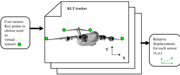
systems. The first step is to record a video of the mechanical system using a high speed digital video camera installed on a fixed point beyond the structure, considered as a fixed point. Then a known length is matched with a pixel correspondence (transform pixels in m). Figure 2 presents the schematics of displacement measurement system using CV techniques.

User mouse: Key points to choose used as virtual sensors Relative displacements for each sensor (xi,yi)

X Y

KLT tracker

Fig 2: Virtual sensor paradigm using KLT tracker. The chosen key points are used as virtual sensor to measure relative displacement frame after frame (sampling frequency is inverse of fps). In our experiment simple plane problems are analyzed in measuring bending displacement (Y in pixel). The true displacement (in m) is obtained from the conversion of a known size part of the structure in pixels.

Firstly the measurement points are selected on the first frame of the video using the mouse with a virtual sensor (i.e. targets; good features to track). The relative displacement of each target is calculated using the optical flow algorithm, which requires good points to track.While analysing image frames, the displacement of the target is calculated (targets motion is in pixels, user must have the true scaling factor). The quantity of information depends on the number of pixels per frame and the number of frames per second. The main advantage of this method is the ability to measure the displacements of multiple locations simultaneously. Moreover in our case there is no aperture problem as the estimated motion is well in the same direction that the real motion (Y displacement). An extension of this paradigm from 2D to 3D have been yet demonstrated in

(11)

measuring three-dimensional motion of a structure using two in-plane measurement systems, which are timely synchronized, and geometrically correlated [18].

3.3. Supervised validation on a simple experiment

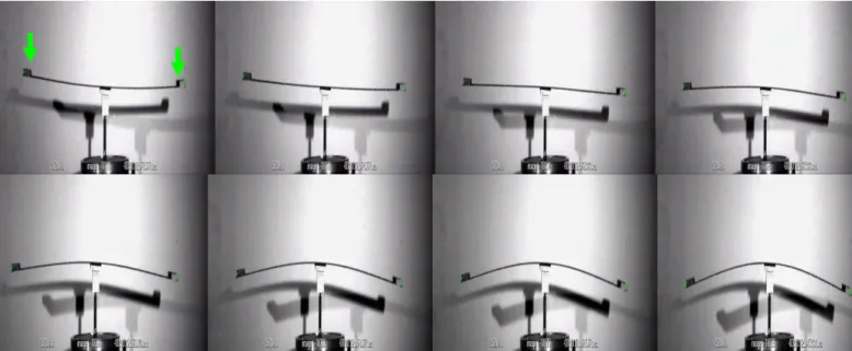
The “Oberst beam” is a classical method to characterize damping in materials. As the base beam is made of a rigid and lightly damped material (steel, aluminium), the most critical aspect of this method is to properly excite the beam without adding weight or damping. A cantilever beam has the same dynamical behaviour as a free-free beam of twice the length, excited at its centre by a normal imposed displacement (Fig. 3). In this case, only the first even mode of the free-free beam will be excited, and its modal behaviour will be similar to a clamped beam since the slope and the relative displacement to the imposed motion are zero at this point. Practically the precision of the location of the centre is important to avoid an unbalanced system [19].

Fig 3: Oberst beam experimental set-up for the free-free beam excited at its centre. Half-period of the first mode is visualized from several successive frames. Virtual sensors are visualized with a small green dot; displacement is measured in Y direction (green arrows).

(12)

Figure 4 shows the measurements estimated by virtual sensors on the two masses at the extremities. It shows a pure harmonic sine, resulting from exciting the first resonance of the

beam. The scale factor associated with this test can be design as

pixels m sf 754 48 . 0 = (1 pixel represents 0.636mm). 0 0.5 1 1.5 2 2.5 -0.03 -0.02 -0.01 0 0.01 0.02 0.03 Time (s) D is p la c e m e n t (m ) left mass right mass

Fig 4: Validation of the algorithm using two virtual sensors on the left (blue line) and right mass (red dot line). The displacement (Y) is measured as a function of time. This displacements have an harmonic form according to the excitation frequency in this experiment close to the resonant frequency which appears at 3.8Hz (period of 0.26s). Figure 5 shows the frequency contents of both virtual sensors which highlight the first resonance mode at 3.8 Hz, which verifies the results found previously by an accelerometer.

0 5 10 15 20 25 30 35 40 45 50 -100 -80 -60 -40 -20 0 20 40 60 Frequency (Hz) S p e c tru m a m p lit u d e ( d B ) left mass right mass

(13)

4. VIRTUAL SENSORS FOR MONITORING AN HELICOPTER BLADE

4.1. Experimental test-rig and pre-processing

For virtual and classical measurement, the experimental set-up is composed of a clamped-free aluminium helicopter blade which is four meters long (Fig 6).

X Y 9 1 Impulsion or shacker

Fig 6: Helicopter blade example: KLT trackers are used to follow 9 targets in bending (Y displacement). The targets

are numbered from 1 to 9, the blade is excited at its center.

The classical experimental equipment used to obtain the modal parameters discussed in this paper is composed on a B&K force sensor 8200 which is then assembled on a shaker supplied by Prodera having a maximum force of 100N. The response displacements are measured with the help of a Laser Vibrometer OFV-505 provided by Polytec. The shaker, force sensor and the laser vibrometer are manipulated with the help of a data acquisition system supplied by LMS Testlab. The center of the blade is excited by burst random excitation (broadband on [0-1600 Hz]). The signal is averaged 10 times for each measurement point. Hanning windows are used for both the output and the input signals. The linearity is checked and a high frequency resolution (∆f = 0.25Hz) for precise modal parameter estimation is used. Response is measured at 40 points that are symmetrically spaced in four rows along the length of the blade. The modal parameters are extracted by a frequency domain parameter estimation method (Polymax).

(14)

For using KLT trackers the blade is excited at its center by an impulsion and the response motion is captured by a high speed camera (Photron Fastcam APX RS3000) at 500 frames/sec. In this experiment, a pixel represents 2.12 mm using a video at a resolution of

1024x256

pixels

(

pixels 47

m 0.1

sf = ), so only the first three bending modes (higher displacements than 2.12 mm) can

be measured. After 30 Hz the others modes (displacements inferior to the resolution) induce only noise. The LK optical flow is used to follow 9 targets (green arrows) in bending along Y displacement. These targets become virtual displacement sensors which allow doing a SIMO analysis in only one test. The main difficulty occurs in signal reconstruction (displacement). Target pixels (which move around x axis) create partial modal data, so displacement signals are irregular data. Thus the small linear displacement hypothesis is used (Fig. 7) to enhance the resolution of the motion and to compensate the missing data. If the absolute value of X (relative displacement on abscissa) is less than 3 pixels the data is used, otherwise it is discarded. According to the figure 7, the virtual sensors vary only in Y direction excepted a small period for KLT 8. So we can say the selected points belong well to a ROI in the image space, so optical flow must be stable for this virtual sensors.

0 200 400 600 800 1000 0 0.5 1 1.5 2 2.5 3 Frame number K L T t ra c k e r X d is p la c e m e n t (m )

Fig 7. Stability diagram: variation of the displacement in X direction are very small function of the frame number (proportional to time vector). So each target vary only in Y direction excepted for KLT 8 (in blue). The virtual sensors are well “attached” to the virtual structure: the points belong well to a ROI in the image space.

(15)

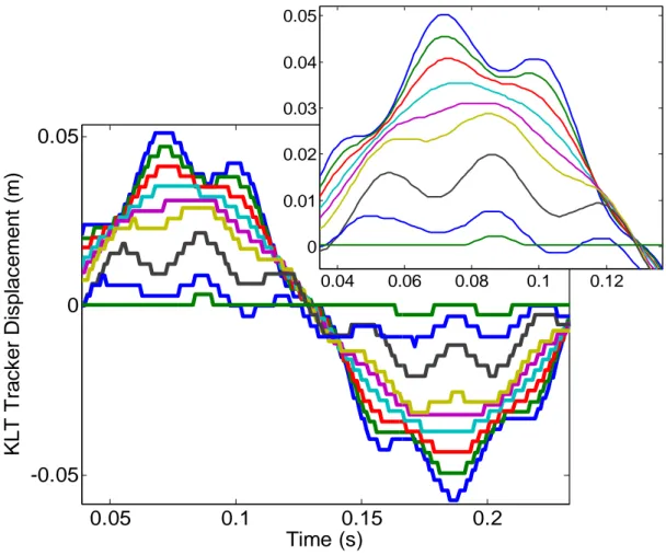
Window functions (Hanning) and low pass filter are applied to the signals. The transfer functions is estimated using tfestimate in Matlab. Figure 8 illustrates the effect of a running moving average (size of the window is 5) on the temporal signals. All these signal processing tools aim at obtaining smoother FRFs for more precise analysis.

Fig 8: Experimental displacements measured on virtual sensors 1 to 9 sampled at FPS. The zoom on the enhanced displacement signaks shows the effect of the moving average function on the temporal signal. This pre-processing aims at obtaining smooth FRFs for better modal parameter estimation.

The type of excitation (smooth impact) offers a correct bandwidth at low frequency which allows the identification of the first three modes. The excitation level which induces the free decay is unknown but we assume that the impulse spectrum is flat on [0-20 Hz] where the 2 identified modes are found. It is clear on Fig 9. that 2 frequencies composed the KLT trackers temporal

0.05 0.1 0.15 0.2 -0.05 0 0.05 Time (s) K L T T ra c k e r D is p la c e m e n t (m ) 0.04 0.06 0.08 0.1 0.12 0 0.01 0.02 0.03 0.04 0.05 Time (s)

(16)

signal. Tracker 1 (in blue) at the free end of the blade exhibits higher displacement than tracker 9 just near the clamped end (in green).

0 0.2 0.4 0.6 0.8 1 -0.06 -0.04 -0.02 0 0.02 0.04 0.06 Time (s) K L T T ra c k e r D is p la c e m e n t (m )

Fig 9: KLT trackers show classically damped sinusoids containing two main frequency. Tracker 1 (in blue) at the free end of the blade exhibit higher displacement than Tracker 9 just near the clamped end (in green).

Due to difficulty to understand our demonstration showing only a sequence of images, videos of this experiment and several others validations are available on the website of the author:

http://personnel.supaero.fr/morlier-joseph/

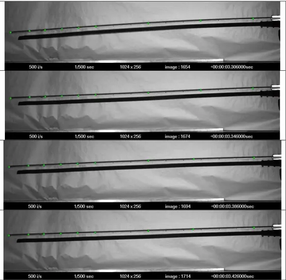
Figure 10 explains the behaviour of KLT trackers showing only a sequence of images: frames 1654-1674-1694-1714 (from top to bottom) of this experiment exhibits one half period of the first mode of the blade. Virtual sensors are visualized with a small green dot; displacements are measured in Y direction (green dots) and correspond to the initial values of KLT trackers of figure 9.

(17)

Fig 10: Half-period is visualized from several successive frames. Virtual sensors are visualized with a small green dot; displacement is measured in Y direction (green dots).

4.2. Comparison of KLT results with EMA and FEM

The results of the FRFs reconstruction permit to realize a classical modal analysis extracting the frequencies, damping ratios and mode shapes. These parameters which characterize the dynamic behavior of the beam are estimated from FRFs using SDOF frequency method called Rational Fraction Polynomial (RFP, [18]) around resonances f_i ±1Hz. Results are listed in table 1.

) f ( E σ( f ) E(ξ) σ(ξ ) 2.32(Hz) 0.2 1.3 (%) 0.02 15.02(Hz) 0.04 0.36 (%) 0.04

(18)

Figure 11 presents filtered FRFs (9 measurement points) and the result of the identification of the first resonance at 3.32 Hz for each transfer functions under the hypothesis of flat excitation spectrum. Thus, the FRF correlation between experimental data and identified data is very good for each virtual sensor.

5 10 15 20 25 30 35 40 45 50 -300 -200 -100 0 Frequency (Hz) F R F m a g n it u d e (d B ) 0 5 10 15 20 25 30 35 40 45 50 -250 -200 -150 -100 -50 Frequency (Hz) R e b u ilt F R F ( m o d e 2 ) (d B )

Fig 11: Filtered FRFs form 9 measurement points and identification of the second resonance at 15 Hz using SDOF RFP method.

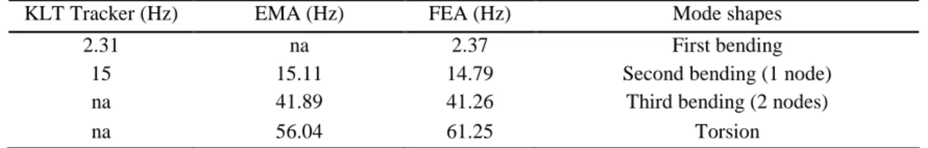
The previous method is compared with classical experimental modal analysis and Finite Element Model. The results are compared Table 2.

KLT Tracker (Hz) EMA (Hz) FEA (Hz) Mode shapes

2.31 na 2.37 First bending

15 15.11 14.79 Second bending (1 node)

na 41.89 41.26 Third bending (2 nodes)

na 56.04 61.25 Torsion

Table 2: Comparison of the estimated frequencies using optical method, classical EMA with burst random excitation (Force sensor not able to detect very low frequency) and Finite Element Analysis using CATIA.

(19)

Using the results of table 2 we can see that KLT tracker method are limited in bandwidth compared to classical EMA (Experimental Modal Analysis) but it offers a simple measurement tool to understand and visualize structural dynamics engineering problems.

The mode shape describes the structure’s motion when it is vibrating at a particular frequency. In the context of SHM mode shape analysis is widely used [22-24] as mode shape is a local parameter which contains spatial information and appears to be more sensitive to the presence of damage zones than natural frequencies. It is also interesting in the boundary conditions analysis or joint characterization [24-26]. The vertical sensitivity is low due to the size of the deflection compared to the length of the beam. It simply allows us to identify only the two first modes with accuracy (Fig. 12); the others displacements are inferior to the pixel resolution.

0.5 1 1.5 2 2.5 3 0 0.5 1 Length (m) N o rm a liz e d m o d e s h a p e ( M o d e 1 ) 0.5 1 1.5 2 2.5 3 0 0.5 1 Length (m) N o rm a liz e d m o d e s h a p e ( M o d e 2 )

Fig 12: Two first mode shapes extracted using KLT on experimental data in black continuous line: The global content of these modes is very close to the two first mode computed using CATIA (red dotted line). Mode 1 is on top of the figure, mode 2 on bottom. The mode shape are normalized in order to be compared to FE modal analysis.

This method can be used according to two other important hypothesis; firstly the number of Frame Per Second (FPS) verifies the Nyquist frequency criteria, secondly the camera axis is perpendicular to the studied 2D structure (to avoid angular errors). One of the limitations is that the influence of the camera viewpoint and calibration has not been taken into account in this study. The other disadvantage is that in some applications the small linear displacement hypothesis is not verified. It induces instabilities of the targets which lead to several partial

(20)

displacement measurements instead of one fixed (x direction) virtual sensor displacement (in bending; y displacement). Nevertheless it offers a simple measurement tool to understand and visualize structural dynamics problems: no targets need to be placed on the structure and several virtual sensors can be tracked simultaneously.

5. CONCLUSIONS

The main goal of this paper is to introduce a practical vibration measurement system developed using available CV tools. KLT trackers are simply used as virtual sensors to measure displacement on video choosing good features to track on the image. The developed method was first validated by using a simple Oberst beam example. Then using several virtual sensors we succeed to estimate the first two main modes of a helicopter blade under impulse excitation. This application can also be used with the help of less expensive tools than high speed camera, e.g. with a classical camera (frequency max is 12.5Hz at image resolution of 1024*768 pixels). One advantage of this non contact measurement method (versus Laser Doppler Vibrometer) is that we can measure in one test several simultaneous outputs for SIMO modal analysis. In order to correct the limitations of KLT tracker, an enhanced version of SIFT (Scale Invariant Feature Transform, [27]) should be developed for 2D structural dynamics application. Finally by the assumptions of high contrast, high vertical resolution (to obtain sufficient deflection) and camera stability, our method coupled with operational modal analysis [28] could also be used to study the flutter behaviour of airplanes under ambient excitation or at a different scale to assess the dynamic parameters of MEMS. Currently work is in progress is to analyse three synchronized video (Multiple camera) for 3D marker less dynamic reconstruction.

(21)

References

[1] S. W. Doebling, C. R. Farrar, M. B. Prime, and D. W. Shevitz, Damage Identification and Health Monitoring of Structural and Mechanical Systems From Changes in their Vibration Characteristics: A literature Review, Los Alamos National Laboratory report LA-13070-MS, 1996.

[2] P. Olaszek, Investigation of the dynamic characteristic of bridge structures using a computer vision method. Measurement 25 (1999) 227–36.

[3] S. Patsias and W.J. Staszewski, Damage detection using optical measurements and wavelets, Vol 1, Structural Health Monitoring, 1 (2002) 5–22.

[4] U.P. Poudel, G. Fu and J. Ye, Structural damage detection using digital video imaging technique and wavelet transformation, Journal of Sound and Vibration 286 (2005) 869–895.

[5] J.J. Lee, M. Shinozuka, A vision-based system for remote sensing of bridge displacement, NDT and E International 39 (5) (2006) 425-431.

[6] J.J. Lee, M. Shinozuka, Real-time displacement measurement of a flexible bridge using digital image processing techniques, Experimental Mechanics 46 (1) (2006) 105-114.

[7] A.M. Wahbeh, J.P. Caffrey, S.F. Masri, A vision-based approach for the direct measurement of displacements in vibrating systems, Smart Materials and Structures, Vol; 12 (5) (2003) 785-794.

[8] J. Morlier, P. Salom, F. Bos, New image processing tools for structural dynamic monitoring, Key Engineering Materials Vol. 347 (2007) 239-244.

[9] Y. F. Ji and C. C. Chang, Nontarget Image-Based Technique for Small Cable Vibration Measurement, , Journal of Bridge Engineering 13 (1) (2008) 34-42.

[10] Y. F. Ji and C. C. Chang, Nontarget Stereo Vision Technique for Spatiotemporal Response Measurement of Line-Like Structures, Journal of Engineering. Mechanics 134, 466 (2008).

[11] J.K. Aggarwal, and N. Nandhakumar, On the computation of motion from sequences of images - A review, in: Proceedings of the IEEE, Vol. 76(8), 1988 , pp. 917-935.

[12] B.D. Lucas and T. Kanade, 1981, An iterative image registration technique with an application to stereo vision, in: Proceedings of Imaging understanding workshop, pp 121-130.

[13] J.L. Barron, D.J. Fleet, and S.S. Beauchemin, Performance of Optical Flow Techniques, International Journal of Computer Vision, 12 (1994) 43–77.

[14] S. Lim, J.G. Apostolopoulos, A.E. Gamal, Optical flow estimation using temporally oversampled video, IEEE Transactions on Image Processing14 (2005) 1074- 1087.

[15] J.Y. Bouguet, Pyramidal Implementation of the Lucas Kanade Feature Tracker, openCV documentation.

[16] J. Shi and C. Tomasi. Good features to track, In: Proceedings IEEE Computer Society Conference on Computer Vision and Pattern Recognition, 1994, pp. 593-600.

[17] Information on http://opencv.willowgarage.com/wiki/

[18] C.C. Chang, Y.F. Ji, Flexible videogrammetric technique for three-dimensional structural vibration measurement, 2007 Journal of Engineering Mechanics 133 (6), pp. 656-664.

[19] J.L. Wojtowicki and L. Jaouen. (2004). New approach for the measurements of damping properties of materials using Oberst beam, Review of Scientific Instruments, 75(8), 2569-2574.

[20] M. H. Richardson and D. L. Formenti, Parameter Estimation from Frequency Response Measurements using Rational Fraction Polynomials, in: Proceedings of the International Modal Analysis Conference,1982, pp.167-181.

[21] H. Wang and W.J. Worley, Tables of natural frequencies and nodes for transverse vibration of tapered beams, NASA CR 443, 1966.

[22] R.D. Adams, P. Cawley, The localisation of defects in structures from measurements of natural frequencies, Journal of Strain Analysis 14 (1979) 49–57.

[23] E. Sazonov, P. Klinkhachorn, Optimal spatial sampling interval for damage detection by curvature or strain energy mode shapes, Journal of Sound and Vibration 285 (2005) 783–801.

[24] J. Morlier, F. Bos and P. Castera, Diagnosis of a portal frame using advanced signal processing of laser vibrometer data, Journal of Sound and VibrationVolume 297 (2006) 420-431.

(22)

[25 N. Olgac, N. Jalili, Modal analysis of flexible beams with delayed resonator vibration absorber: Theory and experiments, Journal of Sound and Vibration 218 (1998) 307–331.

[26 P. Frank Pai, L. Huang, S.H. Gopalakrishnamurthy, J.H. Chung, Identification and applications of boundary effects in beams, International Journal of Solids and Structures 41 (2004) 3053–3080.

[27 Lowe, D. G., Distinctive Image Features from Scale-Invariant Keypoints, International Journal of Computer Vision, 60 (2004) 91-110.

[28 B. Peeters and G. De Roeck, Stochastic System Identification for Operational Modal Analysis: A Review, Journal of Dynamic System, Measurement and Control 123 (2001) 659-667.

(23)

Listing of Figures

Fig 1: Optical flow principle. Pixel motion from image I to image J is estimated solving the pixel correspondence problem: given a pixel in I, look for nearby pixels of the same color in J. Two key assumptions are needed: color constancy (a point in I looks the same in J) and small motion (points do not move very far).

Fig 2: Virtual sensor paradigm using KLT tracker. The chosen key points are used as virtual sensor to measure relative displacement frame after frame (sampling frequency is inverse of fps). In our experiment simple plane problems are analyzed in measuring bending displacement (Y in pixel). The true displacement (in m) is obtained from the conversion of a known size part of the structure in pixels.

Fig 3: Oberst beam experimental set-up for the free-free beam excited at its centre. Half-period of the first mode is visualized from several successive frames. Virtual sensors are visualized with a small green dot; displacement is measured in Y direction (green arrows).

Fig 4: Validation of the algorithm using two virtual sensors on the left (blue line) and right mass (red dot line). The displacement (Y) is measured as a function of time. This displacements have an harmonic form according to the excitation frequency in this experiment close to the resonant frequency which appears at 3.8Hz (period of 0.26s). Fig 5: Frequency contents of the virtual sensors which highlight the expected harmonic mode of the beam at 3.8Hz.