Title
Multiobjective optimization of New Product Development in the pharmaceutical industry
Abstract
New Product Development (NPD) constitutes a challenging problem in the pharmaceutical industry, due to the characteristics of the development pipeline, namely, the presence of uncertainty, the high level of the involved capital costs, the interdependency between projects, the limited availability of resources, the overwhelming number of decisions due to the length of the time horizon (about 10 years) and the combinatorial nature of a portfolio. Formally, the NPD problem can be stated as follows: select a set of R&D projects from a pool of candidate projects in order to satisfy several criteria (economic profitability, time to market) while copying with the uncertain nature of the projects. More precisely, the recurrent key issues are to determine the projects to develop once target molecules have been identified, their order and the level of resources to assign. In this context, the proposed approach combines discrete event stochastic simulation (Monte Carlo approach) with multiobjective genetic algorithms (NSGA II type, Non-Sorted Genetic Algorithm II) to optimize the highly combinatorial portfolio management problem. An object-oriented model previously developed for batch plant scheduling and design is then extended to embed the case of new product management, which is particularly adequate for reuse of both structure and logic. Two case studies illustrate and validate the approach. From this simulation study, three performance evaluation criteria must be considered for decision making: the Net Present Value (NPV) of a sequence, its associated risk defined as the number of positive occurrences of NPV among the samples and the time to market. They have been used in the multiobjective optimization formulation of the problem. In that context, Genetic Algorithms (GAs) are particularly attractive for treating this kind of problem, due to their ability to directly lead to the so-called Pareto front and to account for the combinatorial aspect. NSGA II has been adapted to the treated case for taking into account both the number of products in a sequence and the drug release order. From an analysis performed for a representative case study on the different pairs of criteria both for the bi- and tricriteria optimization, the optimization strategy turns out to be efficient and particularly elitist to detect the sequences which can be considered by the decision makers. Only a few sequences are detected. Among theses sequences, large portfolios cause resource queues and delays time to launch and are eliminated by the bicriteria optimization strategy. Small portfolio reduces queuing and time to launch appear as good candidates. The optimization strategy is interesting to detect the sequence candidates. Time is an important criterion to consider simultaneously with NPV and risk criteria. The order in which drugs are released in the pipeline is of great importance as with scheduling problems.
Key words
Portfolio management, New Product Development, Discrete Event Simulation, Multiobjective opti-mization, Multicriteria Genetic Algorithms
Titre
Optimisation multiobjectif du Développement de Nouveaux Produits dans l’industrie pharmaceutique
Résumé
Le développement de nouveaux produits constitue une priorité stratégique de l’industrie pharma-ceutique, en raison de la présence d’incertitudes, de la lourdeur des investissements mis en jeu, de l’interdépendance entre projets, de la disponibilité limitée des ressources, du nombre très élevé de décisions impliquées dû à la longueur des processus (de l’ordre d’une dizaine d’années) et de la na-ture combinatoire du problème. Formellement, le problème se pose ainsi : sélectionner des projets de R&D parmi des projets candidats pour satisfaire plusieurs critères (rentabilité économique, temps de mise sur le marché) tout en considérant leur nature incertaine. Plus précisément, les points clés récurrents sont relatifs à la détermination des projets à développer une fois que les molécules cibles sont identifiées, leur ordre de traitement et le niveau de ressources à affecter. Dans ce contexte, une approche basée sur le couplage entre un simulateur à événements discrets stochastique (approche Monte Carlo) pour représenter la dynamique du système et un algorithme d’optimisation multi-critère (de type NSGA II) pour choisir les produits est proposée. Un modèle par objets développé précédemment pour la conception et l’ordonnancement d’ateliers discontinus, de réutilisation aisée tant par les aspects de structure que de logique de fonctionnement, a été étendu pour intégrer le cas de la gestion de nouveaux produits. Deux cas d’étude illustrent et valident l’approche. Les résul-tats de simulation ont mis en évidence l’intérêt de trois critères d’évaluation de performance pour l’aide à la décision : le bénéfice actualisé d’une séquence, le risque associé et le temps de mise sur le marché. Ils ont été utilisés dans la formulation multiobjectif du problème d’optimisation. Dans ce contexte, des algorithmes génétiques sont particulièrement intéressants en raison de leur capacité à conduire directement au front de Pareto et à traiter l’aspect combinatoire. La variante NSGA II a été adaptée au problème pour prendre en compte à la fois le nombre et l’ordre de lancement des produits dans une séquence. A partir d’une analyse bicritère réalisée pour un cas d’étude représen-tatif sur différentes paires de critères pour l’optimisation bi- et tri-critère, la stratégie d’optimisation s’avère efficace et particulièrement élitiste pour détecter les séquences à considérer par le décideur. Seules quelques séquences sont détectées. Parmi elles, les portefeuilles à nombre élevé de produits provoquent des attentes et des retards au lancement ; ils sont éliminés par la stratégie d’optimistaion bicritère. Les petits portefeuilles qui réduisent les files d’attente et le temps de lancement sont ainsi préférés. Le temps se révèle un critère important à optimiser simultanément, mettant en évidence tout l’intérêt d’une optimisation tricritère. Enfin, l’ordre de lancement des produits est une variable majeure comme pour les problèmes d’ordonnancement d’atelier.
Mots-Clés
Gestion du portefeuille de produits, Développement de nouveaux produits, Simulation par événe-ments discrets, Optimisation, Algorithmes génétiques multicritères.
1 Introduction, Aims and Scope 11
1.1 General context . . . 13
1.2 Key issues in New Product Development . . . 14
1.3 Portfolio selection . . . 15
1.3.1 Portfolio management definition . . . 15
1.3.2 Risk assessment . . . 15
1.3.3 Objectives of a portfolio analysis . . . 16
1.3.4 Portfolio selection techniques in industrial practice . . . 17
1.4 Related optimization works . . . 18
1.4.1 General classification . . . 18
1.4.2 Presentation of classical approaches for dynamic stochastic open loop method-ologies for NPD . . . 20
1.5 Dissertation outline . . . 22
2 Analysis of New Product Development process 23 2.1 Introduction . . . 25
2.2 Life Cycle of a Pharmaceutical Product . . . 25
2.2.1 A typical pharmaceutical R&D pipeline. . . 27
2.2.2 An example as a guideline . . . 28
2.2.3 Data analysis . . . 32
2.3 Conclusions . . . 34
3.1 Introduction . . . 37
3.2 From batch plant scheduling (BPS) and design to NPD management . . . 38
3.2.1 Model classes . . . 39
3.2.2 Additional classes for NPD modelling . . . 43
3.3 Simulator validation: application to the 9-drug problem of Blau et al. [2004] . . . 45
3.3.1 Simulation for each drug . . . 45
3.3.2 Bubble chart ranking . . . 50
3.3.3 Weighted attractiveness . . . 52
3.3.4 Sequence simulation . . . 53
3.3.5 Conclusion. . . 59
3.4 Resource capacity management . . . 59
3.5 Simulator Validation. Application to Rajapakse et al. [2006] problem . . . 62
3.5.1 Problem description . . . 62
3.5.2 Project management by Discrete event simulation . . . 63
3.5.3 Problem data . . . 64
3.5.4 Simulation results . . . 66
3.6 Conclusions . . . 70
4 Imprecision modelling with interval analysis 73 4.1 Introduction . . . 75
4.2 Imprecision modelling . . . 75
4.2.1 Introduction . . . 75
4.2.2 Probability methods . . . 75
4.2.3 Interval modelling and fuzzy methods . . . 76
4.2.4 Selection of the imprecision modelling technique: interval modelling vs. fuzzy set concepts for NPD problem . . . 78
4.3 Combining discrete event simulation (DES) and interval analysis (IA) . . . 80
4.3.1 Introduction . . . 80
4.3.3 Illustration examples . . . 81
4.4 Extension of the Discrete event simulator for NPD formulation with interval analysis 83 4.4.1 Duration and cost modeled as intervals . . . 83
4.4.2 Parallel activities . . . 83
4.4.3 Net Present Value computation . . . 85
4.5 Simulation example . . . 85
4.5.1 Ideal simulation for each drug (success probabilities equal to 1) . . . 85
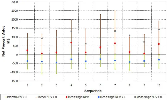
4.5.2 Ideal simulation for 10 sequences (success probabilities equal to 1) . . . 89
4.5.3 Simulation for 10 sequences with success probabilities . . . 89
4.6 Conclusions . . . 92
5 Multiobjective optimization strategies for the NPD process 93 5.1 Introduction . . . 95
5.2 Multiobjective optimization problem formulation. . . 95
5.2.1 General multiobjective optimization problem formulation . . . 95
5.2.2 General optimization methods . . . 97
5.2.3 Multiobjective optimization road map. . . 98
5.2.4 Genetic algorithms . . . 99
5.2.5 Short notes on comparisons of the different non-derivative methods . . . 100
5.2.6 Principles of Non-Sorted Genetic Algorithm II (NSGA II) . . . 103
5.2.7 Combinatorial aspects of the NPD problem and search space definitions . . . . 105
5.3 Implementation of the NSGA II key procedures for NPD modelling . . . 106
5.3.1 Coding, crossover and mutation . . . 106
5.3.2 Optimization parameters . . . 109
5.3.3 Optimization criteria . . . 109
5.3.4 Constraints . . . 109
5.4 Result presentation and discussion . . . 110
5.4.1 Introduction . . . 110
5.4.3 Bicriteria optimization Net Present Value-Makespan . . . 121
5.4.4 Bicriteria optimization makespan-risk . . . 127
5.5 Tricriteria optimization NPV-Duration-Risk . . . 131
5.5.1 Study presentation . . . 131
5.5.2 Conclusion of the bi and tricriteria study . . . 136
5.6 Optimization of a 20-drug portfolio . . . 136
5.7 Conclusions . . . 141
6 Conclusions and Perspectives 143 6.1 Conclusions . . . 145
6.2 Perspectives . . . 147
7 Nomenclature 149 7.1 Nomenclature . . . 151
1.1
General context
Traditionally, Process Systems Engineering (PSE) is concerned with the understanding and devel-opment of systematic procedures for the design and operation of chemical process systems, ranging from microsystems to industrial scale continuous and batch processes. This traditional definition of PSE has been broadened by making use of the concept of the "chemical supply chain" as shown in Figure1.1. Process Systems Engineering is now concerned with the improvement of decision making processes for the creation and operation of the chemical supply chain. More precisely, it deals with the discovery, design, manufacture and distribution of chemical products in the context of many conflicting goals. The area of R&D and Process Operations has emerged among the major challenges in the PSE area: this topics, which has a shorter history than process design and control, expands upstream to R&D and downstream to logistics and product distribution activities.
To support the expansion to R&D, optimal planning and scheduling for New Product Development (NPD) need increased attention to coordinate better product discovery, process development and plant design in the agrochemical and pharmaceutical industries. For downstream applications, areas that receive increased attention at the business level include planning of process networks, supply chain optimization, real time scheduling, and inventory control. Due to the increasing pressure for reducing costs and inventories, in order to remain competitive in the global marketplace, enterprise-wide optimization (EWO) that might be considered as an equivalent term for describing the chemical supply chain (seeShapiro[2001]) has thus become the "holy grail" in process industries.
Figure 1.1: Chemical Supply Chain [Grossmann and Westerberg, 2000]
Enterprise-wide optimization is an area that lies at the interface of chemical engineering (Process Systems Engineering) and operations research. As outlined in Grossmann[2005], a new generation of methods and tools that allow the full integration and large-scale solution of the optimization models, as well as the incorporation of accurate models for the manufacturing facilities is needed. Given the strong tradition that chemical engineers have in process systems engineering and in the
optimization area (seeBiegler and Grossmann[2004] for a recent review), they are ideally positioned to make significant contributions in EWO. This motivates the research challenges of the thesis work, which is devoted to the management of the so-called New Product Development management for pharmaceutical/biotechnology industry. This work is an extension of the investigations previously dedicated to batch plant design and scheduling which are of major importance for such industries and which can be considered as part and parcel of the more general topics of NPD management. Even if this thesis work was not supported by an industrial partnership, it must be highlighted that we have several fruitful discussions with a French pharmaceutical company to assess the validity of the examples that will be tackled here and that will serve as a guideline of the methodological framework.
1.2
Key issues in New Product Development
A fundamental challenge in managing a pharmaceutical or biotechnology company is identifying the optimal allocation of finite resources across the infinite constellation of available investment opportunities. In that context, the optimal management of the new product pipeline has emerged at the forefront of all strategic planning initiatives of a company.
This issue is traditionally identified as a complex one since it integrates various areas such as product development, manufacturing, accounting and marketing. The complexity of the problem is mainly attributed to the great variety of parameters and decision-making levels involved. A strategic investment plan should simultaneously address and evaluate in a proper manner the following four main issues: product management, clinical trials uncertainty, capacity management and trading structure. It is also generally viewed as a multistage stochastic portfolio optimization problem. The main challenge is to configure a product portfolio in order to obtain the highest possible profit, including any capacity investments, in a rapid and reliable way. These decisions have to be taken in the face of considerable uncertainty as demands, sales prices and outcomes of clinical tests that may not turn out as expected.
This kind of problem has recently received attention from the process systems engineering commu-nity utilizing previous works from the process planning and scheduling area. Schmidt and Grossmann [1996] proposed various MILP optimization models for the scheduling of testing tasks with no re-source constraints with a discretization scheme in order to induce linearity in the cost of testing. Jain and Grossmann[1999] extended these models to account for resource constraints. Subramanian et al. [2003] proposed a simulation-optimization framework that takes into account uncertainty in duration, cost and resource requirements and extended this model to account for risk. Maravelias and Grossmann [2001] proposed an MILP model that integrates the scheduling of tests with the design and production planning decisions. A literature review of optimization approaches in the supply chain of pharmaceutical industries can be found in Shah [2004]. The work of Blau et al. [2004] is based on a mono-objective Genetic Algorithm to optimize product sequence evaluated by a commercial discrete-event simulator.
This work lies in this perspective: the underlying idea is to use a multiobjective framework as already initiated by [Aguilar-Lasserre et al., 2007] to model both the conflicting nature of the criteria (i.e. risk minimization and profitability maximization) and the imprecise nature of some parameters (demand, operating times,. . .). In that context, this work aims at the development of an architecture that combines an optimization procedure and a simulation model to represent the dynamic behaviour of the pipeline with its inherent uncertainty and to help decision-making. The general objective is thus to propose a general methodology framework to support decisions and
management of pharmaceutical products involved in their life cycle, from early-stages to mature sales.
1.3
Portfolio selection
1.3.1 Portfolio management definition
Formally, portfolio management is a dynamic decision process, whereby a business’s list of active new product and R&D projects is updated and revised. In this process, new projects are evaluated, selected and prioritized; existing projects may be accelerated, killed or de-prioritized; and resources are allocated or re-allocated to the active project. The portfolio decision process is characterized by uncertain and changing information, dynamic opportunities, multiple goals and strategic con-siderations, interdependencies among projects and multiple decision-makers and locations. Even if portfolio management is viewed as a very important task in industry, there is no consensus about the best strategy, perhaps because there are too many different business practices, much confusion about which strategy is the best, and no easy answers as reported inCooper et al. [1999].
The work presented here has not the ambition to treat all the issues involved but to give a solution to the most critical ones.
1.3.2 Risk assessment
A balanced whole portfolio provides the investor with protections and opportunities with respect to a wide range of contingencies. The investor should build toward an integrated portfolio which best suits his needs [Markowitz, 1959].
A portfolio analysis starts with information concerning individual securities. It ends with conclu-sions concerning as a whole. The purpose of the analysis is to find portfolios which best meet the objectives of the investor [Markowitz, 1959].
Various types of information concerning securities can be used as the raw material of a portfolio analysis. One source of information is the past performance of individual securities. A second source of information is the belief of one or more security analysts concerning future performances. When past performances of securities are used as inputs, the outputs of the analysis are portfolios which performed particularly well in past. When beliefs of security analysts are used as inputs, the outputs of the analysis are the implications of these beliefs for better and worse portfolios [Markowitz,1959]. Uncertainty is a salient feature of security investment. Economic forces are not understood well enough for predictions to be beyond doubt or error. Even if the consequences of economic conditions were understood perfectly, non-economic influences can change the course of general prosperity, the level of the market, or the success of a particular security [Markowitz,1959].
The subject of risk [Kaplan and Garrick,1981] has become very popular and is involved in various fields, far beyond the subject of this thesis: business risk, social risk, economic risk, safety risk, investment risk, military risk, political risk, etc...
Distinction between Risk and Uncertainty The notion of risk involves both uncertainty and some kind of loss or damage that might be received [Kaplan and Garrick, 1981]. Symbolically, it could be written this as:
risk = uncertainty + damage
This equation expresses the first distinction. As a second, it is great to differentiate between the notions of "Risk" and "Hazard".
Distinction between Risk and Hazard In the dictionary hazard is defined as "a source of danger". Risk is the "possibility of loss injury" and the "degree of probability of such loss". Hazard, therefore, simply exists as a source. Risk includes the likehood of conversion of that source into actual delivery of loss, injury, or some form of damage [Kaplan and Garrick, 1981]. This idea is symbolically in the form of an equation:
Risk = hazard saf eguards
This equation also brings out the thought that we may make risk as small as we like by increasing the safeguards [Kaplan and Garrick, 1981] but may never, as a matter of principle, bring it to zero. Risk is never zero, but it can be small.
1.3.3 Objectives of a portfolio analysis
A portfolio analysis must be based on criteria which serve as a guide for the decision maker. The proper choice of a criteria depends on the nature of the investor. For some investors, taxes are a prime consideration; for others, such as non-profit corporations, they are irrelevant. Institutional considerations, legal restrictions, relationships between portfolio returns and the cost of living may be important to one investor and not to another. For each type of investor, the details of the portfolio analysis must be suitably selected [Markowitz, 1959].
Two objectives, however, are common to all investors:
1. They want "return" to be high. The appropriate definition of "return" may differ from investor to investor. But, in whatever sense is appropriate, they prefer more of it to less of it.
2. They want this return to be dependable, stable, not subject to uncertainty.
The portfolio with highest "likely return" is not necessarily the one with least "uncertainty of return". The most reliable portfolio with an extremely high likely return may be subject to an unacceptably high degree of uncertainty. The portfolio with the least uncertainty may have an undesirable small "likely return". Between these extremes would lie portfolios with varying degrees of likely return and uncertainty [Markowitz, 1959]. It must be said at that level that the proper choice among efficient portfolios depends on the willingness and ability of investor to assume risk.
For this purpose, this work must develop a strategy that separates efficient from inefficient port-folios, helps the investor and investment manager to carefully select the combination of likely return and uncertainty that best suit his needs, and finally determines the portfolio which provides this most suitable combination of risk and return.
1.3.4 Portfolio selection techniques in industrial practice
No method has a monopoly in the field of portfolio management. It is quite common that a company uses multiple methods or techniques for portfolio management. These techniques, in rank order of popularity, are as follows [Cooper et al., 1999]:
• Financial methods, where profitability, return, payback, or economic value of the project is determined, and projects are judged and rank ordered on this criterion: 77% of businesses use this approach.
• Business strategy methods, where the business’s strategy is the basis for allocating money for different types of projects. For example, having decided strategy, different buckets or envelopes of money for different project types are established and projects are rank ordered within buckets: 64.8% of businesses use a strategic approach.
• Bubble diagrams, where projects are plotted on on X-Y portfolio map (the X-Y axes are various dimensions of interest, such as reward versus probability of success): 40.6% of businesses employ bubble diagrams.
• Scoring models, where projects are rated or scored on a number of criteria on scales, then the ratings are added to yield a project score (this score then becomes the basis as a rank-ing/prioritizing tool: 37.9% of businesses employ scoring models for portfolio management. • Checklists, where projects are evaluated via a list of yes/no questions (and each project must
achieve all or a certain percentage of "yes" answers): only 20.9% of businesses use checklists for project selection and porfolio management.
The percentage cited add up to well over 100% (241.5%), suggesting that, on average, the typical business relies on about 2.4 times different portfolio management methods. Using multiple methods -the notion of hybrid approach of portfolio management- appears to be the right answer, however [Cooper et al.,1999].
Another kind of classification for studies on R&D portfolio management is considered inWang and Hwang[2007]. Studies on R&D portfolio management can be divided into three categories: strategic management tools, benefit measurement methods, and mathematical programming approaches. The strategic management tools, such as bubble diagram, portfolio map, and strategic bucket method, are used to emphasize the connection of innovation projects to strategy or illuminate issues of risk or strategic balances of the portfolio. Benefits measurement methods determine the preferability figure of each project. A number of approaches, such as the merit-cost value index, the analytical hierarchy process, net present value, and option pricing theory, have been developed in the literature to estimate the benefit of an R&D project. The projects with the highest score may be selected sequentially. The major drawback of most benefits measurements approaches is that neither uncertainty nor resources interactions among projects can be captured. In recent years, some studies used the criterion of conditional stochastic dominance or the mean-Gini analysis to make the decisions to handle R&D uncertainties for risk-averse decision makers.
Mathematical programming models optimize some objective functions subject to constraints re-lated to resources, project logics, technology, and strategies.
The NPD problem is clearly based on an optimization formulation.
1.4
Related optimization works
1.4.1 General classification
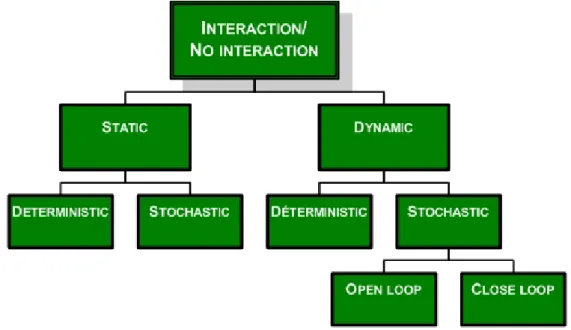
The development of decision support strategies and systems for managing new product portfolios must be able to provide insights to managers on how to minimize risk while optimizing an objective or a set of objectives (e.g. maximization of expected net present value, minimization of time to market, etc.) in the presence of constraints. Moreover, the simultaneous consideration of all candidate projects is the key aspect in managing a NPD pipeline. The complexity of the problem has led to the common use of decomposition based strategies, resulting in two completely independent bodies of decision support literature: strategic/tactical and tactical/operational. Each of the two branches can be further subdivided according to the characteristics of the model used to support the decision making process. A taxonomy is proposed in Zapata et al.[2007]. Figure1.2shows the taxonomy of the main criteria to be considered when characterizing the level of detail of the model used in the decision support strategy for NPD portfolio management.
Figure 1.2: Taxonomy of the level of detail of decision support strategies from Zapata et al.[2007]
The first sublevel reflects the fact that a project can be analyzed in isolation based on certain company standards (e.g. the net present value (NPV) of the project), or as part of the bigger picture where the performance is assessed at the portfolio level (e.g. NPV of the portfolio), including all the interactions between projects. The time dimension is found one level down in the classification. A dynamic model provides the specific state of the systems along each point of the time horizon (e.g. number of projects waiting for resource x at time t), while a static one uses average values to represent the system (e.g. average number of projects waiting for resource x at any time). Within static and dynamic classes it is possible to choose between deterministic and stochastic models. However, dynamic stochastic models have an additional partition: open loop versus closed loop. Open loop models only capture the response of the system to inputs from decision makers, while closed loop models also capture the response of the decision makers to the outcomes from the system.
In the strategic decision support systems literature, the different techniques available are shaped by the type of data used, namely, qualitative and quantitative. Strategies that are based on qualitative data and do not take into account project interactions are static. They have the main objective of translating the vagueness of adjectives used in classifications (e.g. excellent, poor, good, etc.) into structured forms that allow a quantitative comparison of the projects in the portfolio. The methodologies in this area can be grouped into scoring methods [Cooper et al.,1999,Coldrick et al., 2005], analytical hierarchy approaches [Calantone et al.,1999,Poh et al.,2001] and fuzzy logic based approaches [Buyukozkan and Feyzioglu, 2004, Lin and Hsieh, 2004, Lin et al., 2005]. On the other hand, the methodologies that are based on quantitative information strive to provide a realistic simulation of the behavior of each individual project along the time horizon considered, in order to determine what the possible outcomes are in terms of rewards and risk. This group includes dynamic deterministic strategies such as classical financial models (e.g. NPV, internal rate of return (IRR), etc.) ([Cooper et al.,1999], as well as dynamic stochastic strategies, both closed loop such as real options [Copeland and Antikarov, 2001, Loch and Bode-Greuel, 2001, Jacob and Kwak, 2003, Newton et al., 2004, Santiago and Bifano, 2005], and open loop such as discrete event simulation [Chapman and Ward,2002], and neural networks [Thieme et al., 2000]
Most of the approaches that capture project interactions can be classified as dynamic stochastic open loop methodologies. An important contribution is the work of Blau et al. [2004] which proposes the use of stochastic optimization: the portfolio is modeled using a discrete event simulation and the optimization is implemented by a genetic algorithm; Rogers et al. [2002] formulates a real options decision tree that captures technical and market uncertainty as a stochastic MILP that relates projects through a budget constraint. Rajapakse et al.[2005] presents a decision support tool that uses sensitivity and scenario analysis on a discrete event model of the development pipeline. Finally,Ding and Eliashberg[2002] approaches the problem of determining how many projects, that are assigned to develop the same product, have to be included in the pipeline to maximize the total expected profit. For that purpose, they use a static strategy based on a statistical model in which the outcome of each project follows a binomial distribution. All of the techniques in this group are mainly focused on time independent decisions (excluding the work by Rogers et al. [2002]) and therefore do not require closed loop models. Some work has been done to accommodate the higher level of complexity required by time dependent strategic decisions such as capacity expansion/contraction [Wan et al.,2006], but the non-Markovian nature of the associated decision problem has limited such strategies to portfolios with a modest number of projects.
At the operational level, decisions are time dependent. Although their number is substantially larger and their interactions much more complex than those required at the strategic level, they are mostly Markovian in nature (i.e. information about the current state of the system is sufficient to characterize the system and be able to make decisions). This has motivated the development of op-erational decision support systems exclusively based on quantitative information and with a dynamic character. These techniques have mainly focused on scheduling and resource allocation. They can be divided in two main subgroups according to the type of solution strategy, namely conventional optimization and simulation optimization. In the first subgroup the problem is formulated as a re-source constrained project scheduling problem (RCPSP) MILP in which the model is deterministic and the stochastic nature of the system is reflected in the use of expectation in the objective function and constraints. Along these lines,Honkomp[1998] proposed a discrete time MILP formulation that maximizes the total expected net present value of the projects in the pipeline and constrains the allocation of resources based on an overbooking strategy; Jain and Grossmann [1999] presented a continuous time formulation that minimizes the total expected cost of the portfolio and allows the inclusion of outsourcing as an additional degree of freedom in the optimization. The second subgroup determines allocation and scheduling policies by learning from the responses of a discrete event model of the system to changes implemented by a RCPSP MILP [Subramanian et al.,2001,Varma,2005], thus making this technique stochastic.
This work will be devoted to the development of a dynamic stochastic open loop methodology.
1.4.2 Presentation of classical approaches for dynamic stochastic open loop methodologies for NPD
Among the classical approaches, three contributions must be mentioned:
• A formal statement of the portfolio optimization problem is as follows [Blau et al.,2004]: select a set of new drug candidates,and sequence them for the development process in such a way that the economic return expressed as the expected positive new present value (EPNPV) is maximized for a given level of risk measured as the probability of losing money. Let us note at that level that EPNPV is defined as the expected value over the positive axis of the NPV distribution. The information about the negative part of the distribution will be conveyed by using a risk measure called probability of losing money the area under the negative axis of the NPV distribution.
Stated as a mathematical program the portfolio optimization problem is to Maximize EPNPV (over all available drug selections and sequences)
Subject to
P (N P V < 0) < β (Risk constraint)
where β is the risk of losing money.
The methodology proposed byBlau et al.[2004] involves a commercial discrete event simulation tool (CSIM) embedded in a mono-objective optimization tool based on Genetic Algorithms. It can be summarized as follows:
1. An initial list of 10 sequences of drug candidates is generated, some from the bubble chart using individual drug analysis and other at random.
2. For every sequence, the probability distributions associated with the activities for each of its selected drug candidates are modified or are "preprocessed" to account for dependencies between products.
3. The behavior of each sequence is simulated by using a discrete event simulator.
4. The results from these simulations are used by a genetic algorithm to search for improved drug sequences.
The optimization criterion measures how closely the sequence not only maximizes economic per-formance but also minimizes the probability of losing money. The so-called "fitness" function,
Zk, is calculated for each of the candidate sequences in the current population by normalizing
the EPNPV and risk as follows:
Zk = α(
EP N P Vk− EP N P Vmin
EP N P Vmax− EP N P Vmin+ γ
) + (1 − α)( Riskmax− Riskk
Riskmax− Riskmin+ γ
)
where k = 1, 2, . . . , n candidate sequences; EP N V Pmin and EP N V Pmax are the minimum and
maximum expected positive NPV, respectively, in the current population; Riskmaxand Riskmin
are the maximum and the minimum risk probabilities in the current population; and γ is the small positive value that prevents division by zero. The nonnegative number α (between zero and one inclusive) is inversely proportional to the cost per unit violation of the risk constraint, written at a risk tolerance level of β.
• Varma et al. [2008] proposed a framework called SIM-OPT as an integrated resource manage-ment tool with the goals of maximizing the portfolio’s expected net present value (ENPV), controlling risk and reducing drug development cycle times. The framework includes three key components: (1) a stochastic simulation of the pharmaceutical work flow process modeled as a discrete event system, (2) a ”resource manager” based on a mixed integer linear programming formulation that schedules and allocates resources as a function of demands from the simu-lated work process and (3) a ”strategy learner” that evaluates the impact of various resource strategies on the financial and cycle time performance of the simulated pipeline and draws key learnings. The output is a recommended set of resource management strategies and their impacts on expected return, risk and cycle time metrics. Stated as a mathematical program the portfolio optimization problem is to
Maximize ENPV (π)
π ∈Q Subject to
Portfolio risk≤ βRisk
ATM≤ βAT M(i), ∀i ∈ {1, . . . , N }
where π is the optimal policy over the set of all control policiesQ
. The "portfolio risk" can be defined either in terms of P (portfolio NPV < M), where M can be an acceptable loss value or in terms of the standard deviation of the NPV distribution. βRisk is a risk tolerance factor.
The AT Mi is the average time to market for the ith drug and βAT M(i) is the upper bound on
the launch of drug i in the event of clinical success.
• InRogers et al.[2002], a stochastic optimization model (OptFolio) of pharmaceutical research and development portfolio management is presented using a real options valuation approach for making optimal project selection decisions. In this work, only main phases of pharmaceutical R&D are considered: three clinical trial phases, FDA (Food and Drug Administration) approval and product commercialization. According to these researches, one obvious shortcoming of the NPV approach is that it assumes that all future cash flows are static, neglecting the real-world choices to stop investing in the project or change course because of market circumstances. Yet Blau et al. [2004] consider that the Real Options Valuation method has been used effectively only to evaluate single projects.
The problem solved by Rogers et al. can be stated as follows:
Given a set of candidate drugs in various stages of development, estimates of the probability of clinical success, duration, and investment required for the remaining stages and forecasts for the future market values, determine the optimal drug developmental portfolio that maximizes ROV.
Some significant works for dynamic stochastic open loop methodologies for NPD are summa-rized in Table1.1but concern exclusively monocriterion approaches.
This work will be devoted to a combined approach of simulation of the NPD pipeline and strategy optimization. It must be highlighted that the multicriterion feature of the NPD problem must be taken into account and that the various criteria must be thoroughly studied.
Reference Optimization method Criteria
Blau et al. 2004 Genetic algorithm Maximization of Net Present Value Varma et al. 2008 MILP Sim-Opt
Maximization of Net Present Value Risk Minimization
Minimization of average time to market Rogers et al. 2002 MILP Real Options Valuation (ROV) Real Options Valuation Maximization Table 1.1: Summary of classical approaches for dynamic stochastic open loop methodologies for NPD
1.5
Dissertation outline
This introduction (Chapter 1) has presented the key features of the New Product Development problem, the aims and scope of this PhD dissertation.
Chapter 2 describes the activities involved in the NPD problem and the life cycle of a pharmaceu-tical product. A typical pharmaceupharmaceu-tical R&D pipeline serves as a guideline and will be used in the following chapters.
Chapter 3 is devoted to the presentation of the discrete event simulator used to model the various paths and the precedence relations between NPD activities. The simulator extends the previous works carried out in our research group for batch plant design and scheduling. Two case studies are used to validate and illustrate the proposed approach. The uncertainty associated to cost and durations are modeled by probability approaches and Monte-Carlo simulations. The use of a discrete event simulator is particularly useful for decision criteria evaluation, such as economic and risk metrics.
Chapter 4 deals with imprecision modeling involved in the NPD problem. The objective is to investigate alternative approaches to represent imprecision in order to determine the final strategy that could be then selected at the optimization step. An interval-based method is used and the results are compared with those obtained with the probability approach.
Chapter 5 is the core of the methodology: the discrete event simulator is embedded in an outer multiobjective optimization loop. The different optimization methods that may be used are briefly recalled with a special emphasis to Genetic Algorithms (GAs), that are particularly attractive for treating this kind of problem, due to their ability to directly lead to the so-called Pareto front. The test bench examples are analyzed and some guidelines for the treatment of new cases are provided.
Chapter 6 concludes this work by summarizing the main development and results. Possible direc-tions for further research and indicadirec-tions for potential applicadirec-tions are given as well.
Analysis of New Product
Development process
2.1
Introduction
Within the scope of Research and Development Pipeline management problem, several New Product Development (NPD) projects compete for a limited pool of various resource types. The discovery and development of new drugs is a very lengthy and costly process. Each project product usually involves a series of testing tasks prior to product commercialization. If the project fails any of these tasks, then all the remaining work on that product is stopped and the investment in the previous testing tasks is wasted. In this Chapter, we are attempting to present the different steps involved in the process in a generic manner. A flow diagram of the activities involved in the development of a new pharmaceutical product is proposed in Figure2.1. Although some differences may exist referring to various industrial practices, we consider it as generic enough to embed various formulations. Our focus is on providing the key parameters (cost, duration ...) associated with the drug development process. A typical example will serve as a guideline to illustrate the presentation.
Figure 2.1: Process for drugs development.
2.2
Life Cycle of a Pharmaceutical Product
Basically, three stages are involved in the life cycle of a pharmaceutical product: discovery, devel-opment and commercialization as it can be seen in Figure 2.1. In the Discovery stage, thousands of molecules are applied to targets developed to simulate various disease groups. Once an active molecule, i.e. a molecule that is identified to have a curative effect on the target, is discovered, vari-ous permutations of the structure of the molecule are tested to see if the activity can be enhanced. The most active molecule from these structure-activity relationships is tested for toxicological results on rats or mice. If no particular worrisome toxic endpoints are observed, the molecule is promoted to the status of "lead" molecule and becomes a candidate for development.
In the Development stage, enormous sums of money and resources are committed to the lead molecule to first, observe its behavior in healthy volunteers, secondly, in patients smitten with the disease and finally, in large scale clinical studies conducted in concert with the Food and Drug Administration (FDA). Coincident with these studies, process research and formulations work is conducted to both supply the drug for testing purposes as well as to design and construct a commercial plant if the product is launched. Other parallel studies involve extensive long-term (i.e. two years) chronic studies in animals to identify any indication of oncogenicity at different dosage levels.
If the drug is effective in the clinical studies, has no unacceptable side effects and is blessed by the FDA, it moves to the Commercial Stage. Target markets are identified for a staged launch or "ramp-up" of the new compound. After a few years, a mature sales level is usually reached and maintained until patent coverage on the molecule expires and/or competition from generics is realized. Once generics are available, an attempt is usually made to get approval of the drug for alternative markets and perhaps in different dosage forms. Regardless, sales are diminished after expiration of the patent.
2.2.1 A typical pharmaceutical R&D pipeline
In what follows, each stage is described in more details. It must be pointed out at that level that the complexity, creativity and iterative nature of the discovery process make it difficult to describe this step in a high degree of details. Figure 2.2is a simplified network flow diagram of the classical activities involved in the development and commercialization of a new drug candidate.
First human dose preparation (FHDP). This planning activity is relative to the preparation of administration to healthy volunteers. More practically, it includes pharmaco-kinetic studies involving adsorption, distribution, metabolism and excretion from the body as well as determining suitable dose levels.
Phase 1. In this stage, first clinical trials are carried out and drugs are administered to healthy volunteers. At the same time, acute/chronic and reproductive studies are also conducted in animals (mice/rats). Positive results will allow to the drug to go on the process where an unacceptable behaviour in human and animal studies can terminate the study.
Phase 2. Drug is administered to unhealthy human patients with the disease by using the results of dosing studies from Phase I. Coincident with these studies are long-term oncogenic toxicological studies in animals and market research to obtain sales estimates. If the compound fails to treat the disease or is inferior to competitive products, it is de-staged or returned to the discovery phase for modification.
Phase 3. Large-scale clinical studies are carried out on unhealthy human patients. The FDA is involved and indicates benchmarks for giving their approval. In addition to confirming the efficiency, these studies identify drug-drug interactions, human demographics, etc. This most expensive phase of the development process requires extensive global coordination and cooperation. The results should confirm what was learned in Phase II but on a much larger scale, otherwise the compound may be terminated.
First submission for approval. All information (efficacy, toxicology, process, drug-drug inter-actions, side effects, etc.) obtained is gathered and submitted it to the FDA. Simultaneously, the marketing strategy is evolving, price negotiations are being conducted with suppliers/distributors, and promotional materials are being developed. The building of a commercial plant is in progress. Approval for selling the new drug is the anticipated outcome.
Pre-launch activities. This is the final stage before launch-approval has been received from FDA; a global penetration strategy has been completed; the commercial plant has been built and started-up; the promotional campaign launched. This phase ends when the new drug is distributed.
Launch activities. The product is launched over a period of years in various global markets until mature sales levels are reached the ramp-up period. Mature sales are maintained until patents expire or competition is carried out either from competitors or planned cannibalization.
Product supply chain activities. Sample preparation, process research, process development, process design and plant construction occur simultaneously with other development activities (see Figure2.2). Initial focus is on preparing sufficient sample material for various animal/human studies. Once the launch prospects appear promising, the emphasis changes to developing a process for commercialization. This includes a pilot plant which provides data for plant design as well as the larger quantities of material needed for Phase III clinical trials. During Phase III clinical trials, the new plant is designed or other arrangements for product manufacture are carried out. Once Phase III trials are successful, a new plant is needed, existing facilities must be expanded.
2.2.2 An example as a guideline
Typical features
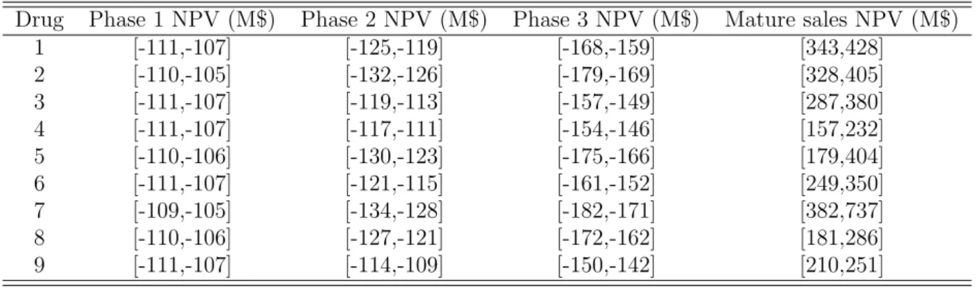
In this section, the example taken fromBlau et al. [2004] is considered as a reference and will serve as a guideline of this presentation. Nine potential new drugs have been identified as lead molecules by the discovery function and are candidates for entering the new product development pipeline. From the flow diagram shown in Figure 2.2, historical data from a major pharmaceutical company were used to represent the parameters with a triangular possibility distribution. The data concerning both duration and cost of each phase are presented in Table2.1. For example, the time required for Phase I testing ranges from minimum (min) of 225 days to a maximum (max) of 375 days with a most likely (ML) value of 300 days; it can be represented by a triangular distribution as shown in Figure 2.3. Costs are not distributed between manpower and equipment/clinical costs. This type of detailed physical resource-based data is generally available and could be used for future resource planning but is beyond the scope of this work. In the last column of Table 2.1, for example, the maximum resources available are specified for each activity. If all the leads are advanced at the same time, the resource levels are exceeded in almost all of the activities. The challenge, therefore, is to propose a strategy, which will mitigate risk while carrying attractive expected financial, since the resources are rarely available to develop all these projects at once.
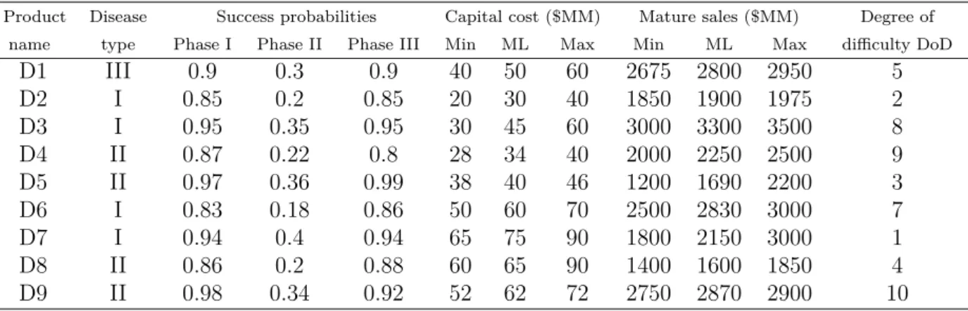
Additional data are provided in Table2.2. The components of and trends in the costs of pharma-ceutical innovation are analyzed in what follows. The example illustrates the interest to diversify a portfolio of new products in order to minimize vulnerability to competitor’s products.
How to obtain economic and technical data
One of the largest components of the overall cost of bringing a new drug to the market is the cost of product development. Cost of product development can account for as much as 30% to 35% of the total cost of bringing a new drug to the market [Dimasi et al., 2003, Suresh and Basu, 2008].
Activity Duration (days) Cost ($MM) Total available resources $MM Min ML Max Min ML Max
FHDP 300 400 500 72 80 88 275 Sample prep 300 400 500 1.8 2 2.2 10 Phase I 225 300 375 70 80 90 350 Phase II 375 500 625 75 80 85 175 Phase III 575 775 975 150 200 250 250 Process develop I 600 800 1000 7 10 13 16 Process develop II 600 800 1000 7 10 13 16 Design Plant 550 750 950 8 10 12 12 FSA 275 375 475 18 20 22 100 Prelaunch 75 100 125 45 50 55 550 Build Plant 600 750 900 52 62 72 120 Ramp up I 250 350 450 9 12 15 25 Ramp up II 250 350 450 19 22 25 50 Ramp upIII 250 350 450 35 40 45 100 Mature sales 250 350 450 46 53 60 150
Table 2.1: Data for Nine Drug Candidates
Figure 2.3: Triangular distribution example
The technical success factors are generally available from researchers while sales/marketing per-sonnel can provide estimates for the sales expected if the compound reaches the marketplace.
For instance, there are three different diseases treated by the nine leads. It would be preferable to treat as many different diseases as possible to minimize the impact of new drugs from competitors sources. Although the drug candidates have never undergone any actual testing beyond the discovery stage, it is often possible to extract subjective probability estimates of their anticipated performance [Morgan and Henrion, 1990, Nutt, 1998] from feedback experience with similar drugs. This remark is also valid for capital cost estimation for manufacturing a candidate drug from the structure of the molecule and the chemical or biological process used to manufacture discovery samples. Finally, market research studies and forecasting practices [Cooper et al.,1999, Kahn,2002] provide price and sales estimates for the product at some launch date in the future. Of course, in all three of these situations, the uncertainty in the estimates is quite large, ranging from 50 to 100 percent of the most likely values.
Product name
Disease type
Success probabilities Capital cost ($MM) Mature sales ($MM) Degree of difficulty DoD Phase I Phase II Phase III Min ML Max Min ML Max
D1 III 0.9 0.3 0.9 40 50 60 2675 2800 2950 5 D2 I 0.85 0.2 0.85 20 30 40 1850 1900 1975 2 D3 I 0.95 0.35 0.95 30 45 60 3000 3300 3500 8 D4 II 0.87 0.22 0.8 28 34 40 2000 2250 2500 9 D5 II 0.97 0.36 0.99 38 40 46 1200 1690 2200 3 D6 I 0.83 0.18 0.86 50 60 70 2500 2830 3000 7 D7 I 0.94 0.4 0.94 65 75 90 1800 2150 3000 1 D8 II 0.86 0.2 0.88 60 65 90 1400 1600 1850 4 D9 II 0.98 0.34 0.92 52 62 72 2750 2870 2900 10
Table 2.2: Success probability, capital cost, mature sales and degree of difficulty
Data source. Based onBlau et al.[2004], cost and duration are taken from a major pharmaceutical company historical data which are used for the simulation. Other practices as market research studies and forecasting are considered too. Capital estimation is carried out by engineers from their experience accumulated from the treatment of similar cases. In the same way, success probabilities are an important parameter considered in NPD evaluation [Morgan and Henrion,1990]. It is important to note that success probabilities are linked to every single product. Success probabilities can be calculated from information about drugs approved by the Food and Drugs Administration or the European Medicines Agency [Reichter, 2001]. An example about how success probabilities can be calculated is applied for monoclonal antibodies (mAbs) which are nature’s biological warheads, able to target and help eliminate foreign or abnormal agents from the body. Table2.3shows data ordered by year and kind of mAbs.
Data were collected from surveys of sponsoring companies, and from public documents. The percentage of completion is the percentage of products that have been discontinued and approved, providing an indication of how far trials have progressed. A low value will inevitably reduce the accuracy of the estimated success rates for that class of mAbs. The percentage of success is the percentage of mAbs that successfully completed trials and were approved by the US FDA, e.g., in Table2.3for years 1992-1994, the total number of mAbs was 41, the number of mAbs discontinued was 23 and the number of mAbs approved was 5; then, the percentage of completion is: (number of mAbs discontinued + number of mAbs approved)/total number of mAbs (23+5)/41= 0.68. For the percentage of success, this is calculated as follows: number of mAbs approved/(Number of mAbs approved + Number of mAbs discontinued) 5/(23+5)=0.18.
Success rates (Table2.4) for phase transitions were calculated as follows: the number of products that completed a given phase and entered the next phase, divided by the total number of products that entered the first phase and did not remain in that phase (i.e., all products entering the phase minus those that remained), e.g., drugs entering (de) to the phase 1:2, drugs completing (dc) the phase 1: 1; the success rate (sr)=dc/de.
Degree of Difficulty. There is a relationship between activity times and costs in Table 2.1 for specific drug candidates. For example, new drugs from a class of chemistries products would require activity resource levels closer to the maximum of the triangular time and cost distributions than those familiar to a company. This relationship is captured with a simple parameter called the degree of difficulty (DoD). Subjective estimates of DoD can be obtained from the various principal investigators, although the values may be different between work processes. However, since the focus of this thesis is on project selection and sequencing rather than resource planning, the analysis can be
Initiation of clinical trials (years) Total number of mAbs Number of mAbs discontinued Number of mAbs Approved % completion % success 1980-1982 2 1 1 100 50 1983-1985 9 8 0 89 0 1986-1988 33 29 2 94 6 1989-1991 34 29 2 91 6 1992-1994 41 23 5 68 18 1995-1997 33 12 0 36 0 1998-2000 34 2 0 6 0 All mAbs (1980-2000) 186 104 10 61 9 Murine mAbs 49 34 1 71 3 Chimeric mAbs 23 13 4 74 24 Humanized mAbs 59 15 5 34 25
Table 2.3: Success rates by year and by product
Initiation of clinical trials (years) Total number of mAbs Number of mAbs discontinued Number of mAbs Approved % completion % success 1980-1982 100 50% 100% 100% 100% 1983-1985 89 67% 50% 50% 0% 1986-1988 94 58% 47% 57% 50% 1989-1991 91 64% 40% 29% 100% 1992-1994 68 85% 55% NA NA 1995-1997 36 77% 55% NA NA 1998-2000 6 90% NA NA NA Murine mAbs 71 77% 52% 45% 33% Chimeric mAbs 74 86% 40% 80% 100% Humanized mAbs 34 84% 72% 75% 100% NA=Not applicable.
simplified by using a single value of DoD ranging from 1 (very easy) to 10 (very difficult). Table2.2 lists DoD for a set of new product candidates. The reported DoD values are used as follows: (1) The minimum and maximum of the triangular distribution remain the same as the values shown in Table 2.1for all the drug candidates; while (2) the most likely value of the distribution is proportional to DoD. If DoD is one, for example, the most likely value is set equal to the minimum of the triangular distribution while the maximum remains the same. Conversely, if DoD is 10 the most likely value is set to the maximum while the minimum remains the same.
The data concerning the example must not be considered in absolute values but represent yet common features observed in this kind of industrial activities.
2.2.3 Data analysis
Basic data
Duration. From the data related to operation duration for the considered fifteen stages (see Table2.1), a triangular distribution has been deduced for representing uncertainty. Let us consider for instance the FHDP activity with a minimum value of 300, a mid value of 400 and a maximum value of 500: 9 possible values are generated (taking into account the number of products to evaluate) from the triangular distribution.
Manufacturing cost. As for duration, data for costs are represented by a triangular distribu-tion.
Resources. For each stage, there is a limited level of available resources for developing drugs projects. This means that the number and order in which drugs projects are initiated then condition the success of a sequence. It is assumed that this constrained resource is renewed after a project has been treated in a step.
Disease type. Three disease types are considered (I, II and III) in Table2.2. Disease of type I involves drugs D2, D3, D6 and D7. Disease of type II is relative to drugs D4, D5, D8 and D9. Disease of type III only involves drug D1.
Success probability. Success probability represents uncertainty related to every drug in stages Phase I, II and III. Given that these stages concern trials, a drug can be rejected or returned for its reprocessing because of inconvenient results in patients. It must be observed that on the one hand, probabilities for phases I and III do not exhibit a big difference between them and are even identical for some drugs. On the other hand, phase II success probability is lower than success probability for phases I and III (this corresponds to the drug test in patients with a disease and outcomes can not be always as desired or expected).
Capital cost. Capital cost is represented by a triangular distribution. A value for the capital cost for a drug will fluctuate between its upper and lower limits established by using a triangular distribution.
Mature sales. As for capital cost, sales are represented by a triangular distribution to model the uncertainty: market behavior is not defined or known in advance due to competition between drugs designed by the same or other companies.
Product dependencies
Product development is generally influenced by the other products considered in the pipeline and by competitor products Roberts [1999]. In some instances, it may be advantageous to manage a candidate drug for early development despite unattractive financial and low technical success probabilities: the gained experience will provide a knowledge base to forecast the success better for dependent drug candidates later in the product sequence.
Traditionally, four frequently occurring types of dependencies are taken into account:
Financial return dependencies. Competition between similar products reduces the profit for each one because of a smaller part of market is gained: this is true for products coming either from the same company or from other ones. This dependency gives a relation for sales taking into account the quantity of products that will arrive until the stage Mature Sales (MS). For a given sequence for the products for the same disease, if two drugs arrive until the stage MS, sales for each drug will be 0.85 of the values for sales reported in Table2.2for every drug. If three drugs arrive until stage MS, sales will be 0.75 of values presented in Table 2.2. Finally, if four drugs arrive until stage MS, sales will be 0.60 of values in Table 2.2(See Table2.5).
Technical dependency. This kind of dependency modifies the success probability. If the first drug in the sequence of drugs targeted for Disease I fails, the probability of technical success for all succeeding drugs decreases by 50%. On the other hand, if the first in the sequence for testing Disease I succeeds, the probability of technical success for all succeeding drugs for Disease I increases by 10%. It must emphasized that this technical dependency is not quite common in the pharmaceutical industry and is even a controversial issue from the fruitful discussions with pharmaceutical managers. This explains why it has not been taken into account for modelling.
Manufacturing cost dependency. Manufacturing cost dependencies occur when the combined cost of a development activity for two similar drug candidates is less than the sum of the cost of the individually considered projects. This has been taken into account in this way: For any sequence of drugs for Disease I, the 1st drug uses full capital shown in Table2.5, the 2nd drug in the sequence uses 1/2 of its individual capital, the 3rd drug uses 1/3 of its capital cost, while the 4th drug uses 1/ 4 of its capital shown in Table2.5.
Resource dependency. Learning effects frequently lead to resource dependencies. A common example occurs when the development times are reduced when taking into account the experience gained by developing two functionally similar drug types one after one.
Disease Drug Type of dependency Disease I D2, D3, D6, D7 Financial dependency
Drug number in the pipeline Percentage reduction of matures sales 2 0.85 3 0.75 4 0.6 Technical dependency Percentage that decreases the probability of success if the first drug in a sequence fails
Percentage that increases the probability of success if the first drug in a sequence succeeds 50 10 Manufacturing cost dependency
Number of drugs Proportion of capital that is used
1 1
2 1/2
3 1/3
4 1/4
Resources dependency Difficulty reduction of 20% due to learning curve experience
Disease II
D4, D5, D8, D9
Financial dependency Total market for drugs of disease II is set at 9000 millions dollars
Technical dependency
Percentage that decreases the probability of success if the first drug in a sequence fails
Percentage that increases the probability of success if the first drug in a sequence succeeds 50 10 Manufacturing cost dependency
Number of drugs Proportion of capital that is used
1 1
2 1/2
3 1/3
Resources dependency Difficulty reduction of 20% due to learning curve experience Disease
III D1
No dependency
Table 2.5: Dependency analysis for the treated example
2.3
Conclusions
This short chapter aims at presenting the typical formulation of New Product Development in a pharmaceutical industrial context: an example serves for illustration purpose. Basically, three stages are involved in the life cycle of a pharmaceutical product: discovery, development and commercial-ization. Our idea is now to use the potential of discrete event simulation to model the series of decision points along the drug development pathway. For example, at the end of each phase of clini-cal trials the probability of cliniclini-cal success resulted in go/no-go decisions. The goal is now to model the pharmaceutical enterprise portfolio by using the principles of discrete event simulation and this is examined in Chapter 3. For this purpose, an object-oriented model structure previously developed for batch plant scheduling and design is extended to embed the case of product management, which is particularly adequate for reuse of both structure and logic.
Development of a discrete event
simulator for the NPD process
.
3.1
Introduction
The goal of this chapter is to model the various paths and the precedence relations between the activities involved in New Product Development by discrete event simulation principles used in previous works for batch plant design [Bérard et al., 2003a,b]. The problem of evaluating and selecting which new products to develop and then of sequencing or of scheduling them is not a trivial task due to dependencies between products both in the market place and in the development process itself. Discrete event simulation is a common tool used to understand how a system works and would work when changes are implemented, without incurring in expensive trials. This technique has thus been chosen and it must be highlighted that experience has been gained in our research group about DES for several years (see for instance the work ofBérard et al.[1999] about batch plant modelling in the pharmaceutical industry). DES development has shown that its internal structure and its performances were well fitted for the problem under consideration. This is why DES has been considered as the basic tool for the present work, even if some modifications and adjustments are necessary to obtain an efficient tool to tackle the NPD pharmaceutical projects of this study.
Some investigations [Blau et al., 2004, Rajapakse et al., 2005, 2006, Varma et al., 2008] used commercial simulation software tools based on discrete event simulation (CSIM 1, Simulator Ex-tended Industry Suite V5, GenSight software2, ...) with specific advantages. However, limitations of graphically based simulators to interact with other applications, has forced us to develop our own simulators.
This explains our main motivation to use and adapt the simulator previously developed in the group, taking into account our background on this topics since 1992 (defense of ten PHD thesis, more than 22 international publications on the subject). The C++/implemented DES can be easily modified for modelling the NPD problem considered here. This constitutes the first step of a general framework for managing NPD projects that will consider the integration of this simulation tool in a more general-purpose simulation-optimization perspective.
This chapter involves three sections:
• The extension of the DES previously developed for batch plant scheduling to the NPD problem is first presented;
• A typical simulation analysis is then performed using the example derived from [Blau et al., 2004] involving nine drugs and three target diseases. The drugs are first analyzed independently via the so-called bubble chart. Then, the interest of simulation is justified for drug sequences. The influence of capacity limitation is also highlighted.
• Another example is also considered to show the capability of the model to take into account various situations [Rajapakse et al., 2006] and to demonstrate its interest as a stand-alone decision aid tool.
1
http://www.mesquite.com
2
3.2
From batch plant scheduling (BPS) and design to NPD
man-agement
In a DES, a process is described as it evolves with time and changes take place only a finite number of times, i.e. event occurrence date. The DES was developed using C++ object-oriented language, according to the approach proposed byBérard et al.[1999] (Figure3.1). It must be emphasized that object-oriented (OO) techniques have received a lot of attention in recent years and the use of OO techniques are becoming increasingly common. The power of object oriented techniques lie in the ability to produce "modular" code (known as classes) that can be "easily" modified and reused. The ability to contain software complexity into classes and to be able to realistically represent entities from the real world in software makes OO techniques ideally suited to simulation which is inherently complex.
InBérard et al. [1999], a four layer framework was proposed based on the following items engine, event, object, supervisor, the aim being the development of a standard library for the simulator classes that are general to any case, thus minimizing the task of treating different study cases or the variants of a given one (i.e. design or scheduling objectives). In this approach, at the lowest level, the common engine can be found. Initially, the events in the next level are generic events common to all batch plant simulations: in this case, the definition must be adapted since we have to consider the whole life cycle of a project related to a product. In the same way, the objects taken into account present some similarities but differ in their appreciation: for instance, in batch plant scheduling problems (BPS), material resources are constituted by equipment whereas in NPD problems, resources may be viewed more globally. In fact, the main differences at this step occur from a terminology point of view and this can be easily transposed in the NPD formulation (see Table3.1).
Figure 3.1: DES Framework.
In what follows, the description of the basic design of the DES and its operation principles are presented. Following the classical terminology used in object-oriented approaches, the main so-called objects of the DES will be described. To treat a particular problem, specific objects should be derived from this basic structure.