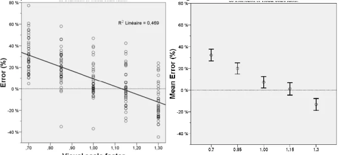
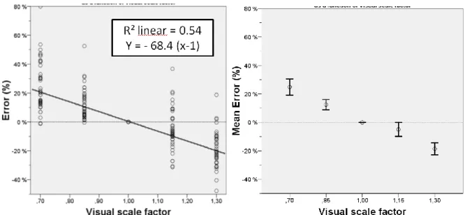
Visual Scale Factor for Speed Perception
Texte intégral
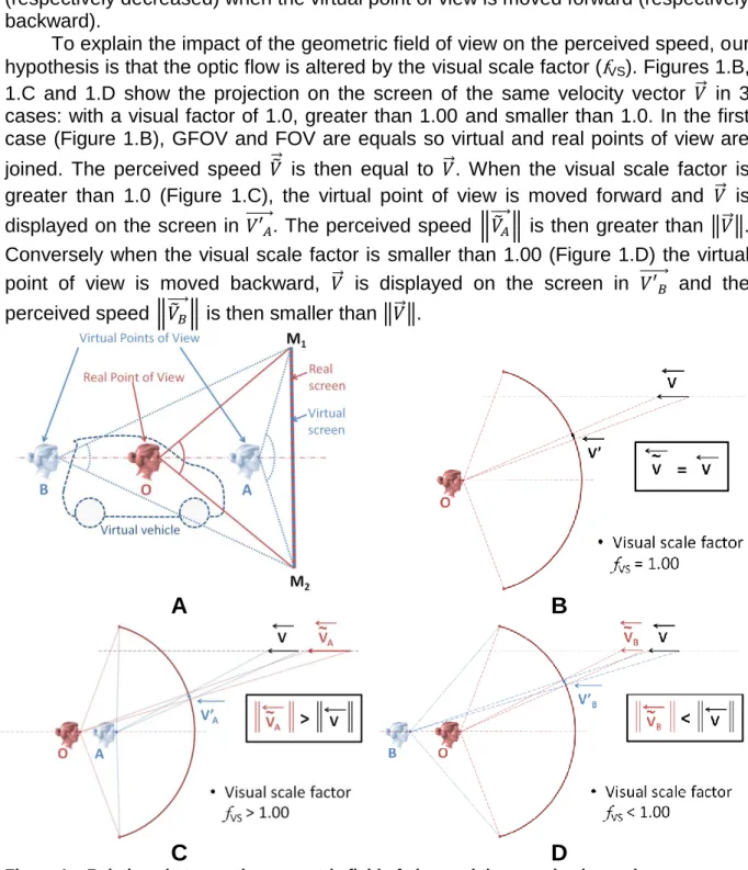
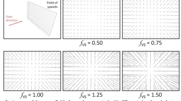
Figure

Documents relatifs
Beide Länder weisen einen geringen Versorgungsgrad bei ausserhäuslichen Dienstleistungen für Kinder im Alter von bis drei Jahren auf, sind geprägt durch eine geringe
Einstein gravity with extra dimensions or alternative gravity theories might suggest that the gravity propagation speed can be different from the light speed). Such a difference
Numerical analysis of the topological gradient method for fourth order models and applications to the detection of fine structures in imaging. Topological gradient method applied to
We have discussed in this paper the speed of approach to equilibrium for a colli- sionless gas enclosed in a vessel whose wall is kept at a uniform and constant tem- perature,
The discrepency between the effective strengths of the pore pressure and saturated rocks at high strain rates indicates that the computed effective confining pressure
Downes,David Martson and Inci Otker , Mapping Financial Sector Vulnerability in non Crisis Country IMF Discussion Paper 1999.. (2) Mannuel Hinds, Economic Effects of
Cuperlovic-Culf, Mira; Wang, Lipu; Fobert, Pierre; Rajagopolan, Kishore; Loewen, Michele; Li, Forseille; Boyle, Kerry; Merkley, Nadine; Burton, Ian; Foroud, Nora; Hazendonk,
pneumophila must also prevent mitochondrial apoptosis to promote replication, as loss of pro- survival BCL-2 family members, BCL-XL and MCL-1, induces cell death of infected
