is an open access repository that collects the work of Arts et Métiers Institute of Technology researchers and makes it freely available over the web where possible.
This is an author-deposited version published in: https://sam.ensam.eu
Handle ID: .http://hdl.handle.net/10985/8548
To cite this version :
Christophe GIRAUDAUDINE, Frédéric GIRAUD, Michel AMBERG, Betty LEMAIRESEMAIL -Vector control method applied to a traveling wave in a finite beam - Ultrasonics, Ferroelectrics, and Frequency Control, IEEE Transactions on - Vol. 61, n°1, p.147-158 - 2014
Any correspondence concerning this service should be sent to the repository Administrator : archiveouverte@ensam.eu
0885–3010 © 2014 IEEE
Vector Control Method Applied
to a Traveling Wave in a Finite Beam
Frédéric Giraud, Member, IEEE, christophe Giraud-audine, Member, IEEE, Michel amberg,and Betty lemaire-semail, Member, IEEE Abstract—This paper presents the closed-loop control of
exciters to produce a traveling wave in a finite beam. This control is based on a dynamical modeling of the system es-tablished in a rotating reference frame. This method allows dynamic and independent control of the phase and amplitude of two vibration modes. The condition to obtain the traveling wave is written in this rotating frame, and requires having two vibration modes with the same amplitude, and imposing a phase shift of 90° between them. The advantage of the method is that it allows easy implementation of a closed loop control that can handle parameter drift of the system, after a tempera-ture rise, for example.
The modeling is compared with measurement on an experi-mental test bench which also implements real-time control. We managed to experimentally obtain a settling time of 250 ms for the traveling wave, and a standing wave ratio (SWR) of 1.3.
I. Introduction
r
esearchers have devised many applications for high-frequency traveling waves. For example, they can convey a small carriage over a stator rail in a linear motor [1]–[3]. In that case, the elliptical motion of the vi-brating stator drives the mechanical load directly, which is a simple solution compared with a rotary-to-linear move-ment transformation stage. They also can be used in peri-staltic pumps [4] because the traveling wave micropumps are then free of rubbing parts. a traveling wave in a small cylindrical tube can also be obtained, and sun et al. [5] used a combination of radial and axial modes of the tube, with specific driving conditions.In general, the mechanical arrangement of such sys-tems is quite simple. In fact, two exciters are used, one produces the vibration and the other absorbs the reflected wave. By swapping the role of the two exciters, a traveling wave in the reverse direction is obtained. However, to real-ize this, some conditions must be fulfilled, or no traveling wave propagates. These conditions have been studied in many papers. For example, Kuribayashi [6] described a
methodology to design the system, to choose the beam length and where to place the exciters on the beam. He also connected a resistor to the second exciter to dissipate the energy of the propagated wave. However, the practi-cal realization of this solution suffers from poor efficiency, because a large amount of energy is lost into the resistor.
Therefore, some authors prefer an active sink instead [7]. In that case, the tuning of the exciters—their supply voltage, frequency and phase shift—becomes complex to obtain the traveling wave. The analytical solutions for a traveling wave in a string, a beam, and a membrane are given in [8]; the authors calculate the analytical expression of the applied forces to obtain a pure traveling wave in an undamped medium. They also show that it is sufficient to excite ten modes only; the other modes’ contribution can be neglected. In [9], dehez et al. proposed an optimization procedure. For their study, they first choose two neighbor-ing vibration modes, which should be prominent. Then, they calculate the participation factors of a finite number of vibration modes above the chosen ones. They adjust their parameters through an optimization loop so as to make those factors as close as possible to those of the Fou-rier series coefficients of a square wave. In [10], Minikes et al. developed methods for identification and tuning of the traveling wave, or for multiple traveling waves [11]. They used a sensor array to measure the deformation amplitude and phase at specific points, then, an ellipse is fitted to the graph in the complex plane. If a pure traveling wave is obtained, then the fitted ellipse becomes a circle. once again, they adjust the values of the excitation parameters through an online optimization process to reach the ideal case.
These methods can be off-line [8], [9], which means that the excitation is calculated before the experimental runs, or on-line [10] and can thus adapt themselves to variation in the operating conditions. However, their tuning proce-dure is based on steady states, and dynamic performances are not studied.
The method presented in this paper proposes to dy-namically tune the two exciters to obtain a traveling wave in a slightly damped beam. The control algorithm relies on a model which is obtained from the theory of vibration in a beam, and which is detailed in the first section of this paper. after having verified this model through an experi-mental study, we establish this model in a rotating refer-ence frame, to obtain constant-state variables at steady state. a specific closed-loop control is then deduced for our application, the performances of which are experimen-tally verified.
Manuscript received May 10, 2013; accepted september 26, 2013. This work was carried out within the framework of the stimtac Project of the Institut de recherche sur les composants logiciel et matériels pour la communication avancée (IrcIca), and the Mint team of InrIa lille nord-Europe.
F. Giraud, M. amberg, and B. lemaire-semail are with the Institut de recherche sur les composants logiciels et matériels pour l’Information et la communication avancée (IrcIca), Université lille 1, Villeneuve d’ascq, France (e-mail: frederic.giraud@polytech-lille.fr).
c. Giraud-audine is with the Ecole nationale superieure d’arts et Metiers, Villeneuve d’ascq, France.
II. Beam Theory A. Mode Shape
In this study, we consider the forced vibration of the finite beam shown in Fig. 1. The transverse vibration of a uniform elastic homogeneous isotropic Euler–Bernoulli beam is described by the following differential equation [12]: EI w x A w t r w t p x t a ∂ ∂ + ∂ ∂ + ∂ ∂ 4 4 2 2 = ( , ) ρ , (1)
where E is the young’s modulus of the beam, I is the quadratic momentum of the beam, A is the cross section and ρ is the mass per unit volume of the beam, ra is a coefficient of the external damping, w(x) is the beam’s deflection at point x and time t, and p(x, t) is the load per unit length.
With a pure harmonic and concentrated excitation, the load p is written as p(x, t) = F xδ( x e) j tω
1
− , where δ(x) is the dirac’s delta function and j2 = −1. The deflection is then considered as purely harmonic, and if we introduce w
such that w is the real part of w, we can write
w x t( , ) =W t x e( ) ( )Φ j tω. (2)
In (2), W includes both amplitude and phase of the deflec-tion of the vibradeflec-tion. We should note that although ω is constant in the study, W t() may vary with time. Thus, we not only consider the steady operation, but the transient as well. Moreover, w is given for the deformation shape of the vibration Φ(x) which is normalized. Eq. (3) shows an example of a condition of normalization of the mode shape: 0 2 ( ) = 1 L A x x
∫
ρ Φ d . (3)The solution of (1) can be found in [9], [12], and will not be discussed in this paper. We note however, that we can analytically calculate the deflection for a particular posi-tion, as presented in Fig. 2. In this figure, we depict the deflection calculated at x = 0.29 m for an aluminum beam of 6 × 6 mm cross section and with L = 0.48 m. We also
depict the experimental response of the beam, which is measured with a laser interferometer.
The analytical and experimental responses do not ex-actly match, despite some parameter adaptation done for this figure. This is mainly due to the analytical model-ing, which considers an Euler–Bernoulli beam, which is not completely verified. However, differences are accept-able within the scope of this paper, because the proposed control doesn’t require accurate parameter estimation. Furthermore, we show that beam’s deflection has maxi-mum values for particular excitation frequencies. These frequencies are known as eigenfrequencies, for which the beam has a specific shape, the so-called normal mode or modal shape. These deformation mode shapes refer to the function Φn(x), and they can be found either from analyti-cal study, or more conveniently, from finite element model-ing. Fig. 3 presents the deformation mode shapes for the two modes at 17 500 and 19 440 Hz (analytical).
actually, under normal load excitation, every vibration mode is excited in the beam, but with different deflection, namely Wn. Eq. (2) is, in fact, an approximation of the beam’s deflection around the vibration modes, and must be changed to w x t W x e n n n j t ( , ) = ( ) =1 ∞
∑
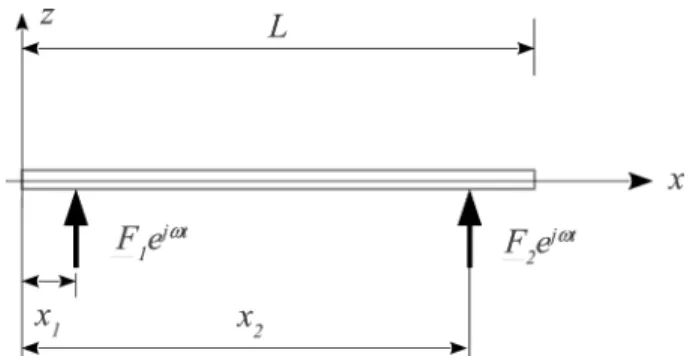
Φ ω. (4)The deflection Wn depends on frequency. For example, they are maximal for the eigenfrequency ω0n and the de-formation which is then obtained corresponds to the func-Fig. 1. The studied beam is supposed to be free at its ends and a
sinu-soidal load F t() is applied at x = x1. Fig. 2. deflection amplitude as a function of frequency at x = 0.29 m with x 1 = 0.196 m and L = 0.48 m; comparison with experiment.
tion Φn(x). Fig. 4 shows the deflection Wn for the mode at 19 440 Hz. as can be seen, this deflection follows the fre-quency response of a resonating low-pass filter: it is almost constant for ω < ω0n and then drops to 0 for ω > ω0n.
Hence, the participation of a mode to the deformation of a beam is dominant if the working frequency is close to the eigenfrequency of this mode (i.e., ω = ω0n), significant if the working frequency is lower than this eigenfrequen-cy (i.e., ω < ω0n), and negligible for working frequencies above the eigenfrequency (i.e., ω > ω0n). This property is important and will be used later in this paper.
B. Conditions to Obtain a Traveling Wave
To produce a traveling wave, a second exciter is placed on the beam at distance x2. This configuration is described in Fig. 5.
Under certain supply conditions of the two exciters, it is possible to obtain a traveling wave. These conditions include adequately choosing the supply pulsation ω and the two forces F1 and F2.
In principle, the idea is to use two neighbor modes a and b and to excite these two modes simultaneously, but shifted in time by 90°. In fact, when we consider the two deformation shapes in Fig. 3, we observe that they are close to sinusoidal shapes, and that they are almost space shifted by 90°, roughly in the region 0.2 m to 0.3 m in the middle. This condition can lead to a traveling wave, as presented in [10]. To obtain the two modes, we choose ω between the two eigenfrequencies: the lower mode is not too attenuated, whereas the higher one is significant.
These two modes are necessary, but not sufficient. In fact, we observe in the same Fig. 3 that the two modes are not phase shifted by 90° near the end of the beam. conse-quently, if they were alone, they would not produce any traveling wave in that region. However, experimental stud-ies in literature reported a traveling wave between the two exciters, and not only in the middle of the beam. This consideration illustrates the effect of the modes above the two chosen ones. dehez et al. [9] have shown that they have influence in the ends and not in the middle of the beam. In this paper, we will consider that if the two modes a and b have the same amplitude and are phase shifted by 90° (Wa = jWb), a traveling wave in the beam results. However, Gabai and Bucher [8] point out that perfect
traveling wave is obtained when a large number of modes is taken into account; then, we expect to have an imper-fect traveling wave in our case. This point will be quanti-fied by experimental tests.
studies reported in the bibliography do not control the two modes a and b directly: F1 and F2 are tuned until a perfect traveling wave is obtained, through an optimiza-tion algorithm, for instance. In this paper, we propose a method to directly control the two vibrations of the two modes a and b. This control relies on a model which is first presented, and then the control scheme is deduced and implemented on an experimental test bench.
III. dynamic Modeling of the Beam
The purpose of this section is to propose a model which allows us to calculate the evolution of the vibration ampli-tude of the modes a and b, and the phase shift between the two modes. In this section, we first apply beam theory to obtain a model which is confirmed by simulation results. A. Modeling in a Fixed Reference Frame
This section deals with the evolution of the instanta-neous vibration amplitude for the two modes. For that purpose, let w tk( ) = W t ek( ) j tω, with k = {a, b}. This is
equivalent to considering w tk( ) as a rotating vector in a fixed frame, as depicted in Fig. 6. The length of this vector is Wk , and the projection on the real axis is the actual value which can be measured experimentally. Finally, the difference of the arguments of W tk( ) represents the phase shift between the modes.
Fig. 4. calculated deformation Wn as a function of frequency for the
mode at 19 440 Hz. Fig. 5. The beam and its exciters to produce a traveling wave.
Projecting (4) onto each mode [13], we obtain 0 4 4 0 2 0 2 ( ) ( ) ( ) ( ) ( ) L k k k a L k k L k EI x d x dx xw t r x xw A x x w
∫
∫
∫
+ + Φ Φ d Φ d d ρ φ kk = L k( ) ( , )x p x t x k { , }a b 0∫
Φ d , ∈ . (5)For sake of simplification, we define: • the modal mass mk = ρA
∫
0LΦk2( )x xd ,• the modal damping dsk = ra
∫
0Lφk2( )x xd , and• the modal stiffness ck = EI
∫
0LΦk( )x((d4Φk( )x) (/ dx4)) .dxThe participation Ka1 and Ka2 of each force F1 and F2 for mode a are defined as
0 1 1 2 2 1 1 2 2 ( ) ( , ) = ( ) ( ) = ( ) L a a j t a j t a a j x p x t x x F e x F e K F K F e
∫
+ + Φ d Φ ω Φ ω ω ω ω t a j t F e = . (6)Hence, the participation of F1 and F2 is equivalent to the participation of a virtual modal force Fa = (K Fa1 1 +
K Fa2 2). In the same way, we define Fb = (K Fb1 1 + K Fb2 2).
This shows the importance of localization of the actuators. Indeed, if they are placed in locations such that Φa(x1) = Φa(x2) = 0, it becomes impossible to excite the mode a. of course, the same conclusion holds for mode b. Finally, we introduce the matrix Kab, defined by
F Fab abxx abxx FF Kab FF
( ) (
= ( )( )1 ( )( )2) ( )
. =( )
1 2 1 2 1 2 Φ Φ Φ Φ . (7)according to these definitions, (5) is then revised into
m wa a +d wsa a +c wa a =F ea j tω. (8)
In the same way, we obtain for the mode b
m wb b +d wsb b +c wb b =F eb j tω. (9)
Finally, the vibration amplitude for the two modes, and their phase shift, can be calculated using (8) and (9), by
W tk( ) =w ek − ωj t. (10)
Hence, (6), (8), and (9) describe the evolution of the vibration amplitude for the two modes a and b. These equations yield a model which can be represented by way of a causal ordering graph (coG), as shown in Fig. 7. In principle, only equations using integral relations (ellipses with single arrow) or relations independent of time (el-lipses with double arrow) can be used [14]. Hence, the equations are revised into
• RK: Fk =K Fk1 1+K Fk2 2, • Rθ : fa =Faej tω, fb =Fbej tω, • Rk1: w k m f f t k k ek = 1
∫
( − )d , • Rk2: fek =ck∫
w t kd , • Rθ−1:W w e k = k − ωj t, with k ∈ {a, b}.To validate the model, we compare in Fig. 8 measure-ments on the aluminum beam to the model. We compare the actual value of w(t), which is sinusoidal, and the simu-lated value of the deflection amplitude W(t) which repre-sents the amplitude of w(t) (see appendix a for a descrip-tion of the test bench). The measurements on the beam were made with a laser interferometer which measures the vibration speed instead of the deflection. We thus compare
w x t( , ) for the simulation and the experimental study when F2 = 0 and F1 is step varying. For the three runs, the ex-perimental conditions were:
• case a: the frequency corresponds to the eigenfrequen-cy of mode a and the step value for F1 = 1N,
Fig. 7. The causal ordering graph of the system.
Fig. 8. comparison between modeling and the experimental output at
• case c: the frequency corresponds to the eigenfrequen-cy of mode b and the step value for F1 = 1N,
• case b: the frequency is at the middle of modes a and b, with a step value for F1 = 3N.
The other parameters of simulations are kept constant. The simulation is found to be consistent with the ex-perimental study, validating the approach. However, this modeling is established in a fixed frame, and state vari-ables are sinusoidal functions of time. However, in this paper, we are interested in the evolution of the deflection amplitude and the phase shift of these variables. This is why, in the next section, the modeling is modified, and presented in a rotating reference frame.
B. Modeling in a Rotating Reference Frame
We have defined wk as two complex numbers. conse-quently, Wk are the coordinates of wk in a rotating refer-ence frame attached to ejωt. The rotating reference frame
is named (d, q) and is attached to ejωt as shown in Fig. 6.
For steady-state operation, Wk are constant; hence, the affixes of wk are along a circle in the fixed frame. However, for the most general case, Wk depend on time and the positions of their affix vary in the rotating frame.
The purpose of this section is to obtain the dynamic of
Wk directly, without calculating wk for the general case. We first calculate each derivative of wk:
d dwtk = (j Wω k + W ek) j tω, (11) and d d 2 2 = ( 2 2 ) w t k −ωWk + j Wω k +W e k j tω. (12)
substituting (11) and (12) into (8) leads to
m W d m j W c m j d W K F a a sa a a a a sa a a a + + + − + ( 2 ) [( 2) ] = ω ω ω , (13)
where we also simplified left and right by ejωt. This
equa-tion is linear and can be solved, because ω is constant. However, for the sake of simplification, we make the as-sumption that W a ≪ ω Wa and W a ≪ ω Wa ; this can be acceptable if the dynamic of Wa is limited by ω. Then, the terms d Wsa a and m Wa a can be neglected, compared
with d Wsaω a and m Waω ,a respectively. one consequence is that the closed-loop dynamic proposed in this paper will have to be tempered to fulfill this condition. Finally, (13) can be simplified into
2m j W [(c m 2) j d W] =K F
a ω +a a − aω + ω sa a a a. (14)
We now project (14) onto axes d and q of the rotating frame. For that purpose, we define Wa = Wad + jWaq, and Fa = Fad + jFaq, as illustrated in Fig. 9.
Moreover, we separate the imaginary part and the real part of this equation, leading to two new equations:
−2m W −d W =F −(c −m 2)W
aω aq saω aq ad a aω ad (15)
2m W d W =F (c m 2)W
aω ad + saω ad aq− a − aω aq. (16)
as can be seen, this model can be explained as follows: • Fad controls Waq, and Wad produces a perturbation, • Faq controls Wad, and Waq produces a perturbation. Moreover, for steady state operations, W aq = 0 and W ad = 0, and hence, Fad and Faq are constant over time.
a new coG is drawn in Fig. 10, where Rad refers to
(15) and Raq to (16). We also represented the equation
for mode b, Rbd and Rbq being given for similar equations.
This model is then compared with simulation in Fig. 11 for a step variation of F1 from 0 n to 3 n. We have chosen the frequency corresponding to mode a, and then to mode b; indeed, for these frequencies, the cross-cou-pling between axes d and q is removed, yielding a first-order type response to step variation of the forces. This is clearly confirmed by the experimental test, which shows responses close to the model.
The advantage of this model is to use variables which are constant at steady state, and not sinusoidal functions of time. This makes the control easier, and we can now de-vise controls imposing the amplitude and phase of the two modes a and b. The next section presents such a control. Fig. 9. representation in a rotating reference frame.
IV. control of the Traveling Wave A. Control of Wa and Wb
The working frequency is fixed, and chosen between the eigenfrequency of the two modes. We must control Fkd and Fkq to obtain
Waref = jWbref (17) automatically. In this way, no optimization loop is neces-sary at this point to obtain the traveling wave. Hence, the four vibration amplitudes must be controlled.
First, we choose to align the rotating frame on mode a. This condition leads to Wadref = 0 and Waqref = W, and
also Wbdref = W and Wbqref = 0. The position of the
ampli-tude reference can be represented in the rotating reference frame, as depicted in Fig. 12.
Four control loops are needed, two for mode a (axes d and q), and two for mode b (axes d and q also). Integral-proportional controllers are used. The decoupling of the two axes is achieved by imposing very different settling times: the dynamics of Wbd and Waq are set faster
com-pared with the dynamics of Waq and Wbd, respectively, to align the vectors Wa and Wb on their axes.
The closed-loop control of mode a is thus represented in Fig. 13, and for purpose of illustration, we give in (18) the computation of the force Faqref for the amplitude reference along axis q of mode a, Waq, with s the laplace variable:
Fda Kpaq T s W W
aq aq aq
ref = 1+ 1 ( ref − ). (18)
Finally, the input forces F1 and F2 are calculated using (7), giving: F F K F jF F jF ab ad aq bd bq 1 2 1 =
( )
+ + − ( ) ref ref . ref ref (19)B. Experimental Results of the Control of Modes a and b For the beam under study, we have chosen the mode a at f = 17900 Hz and the mode b at f = 20 200 Hz. We have fixed the working frequency in the middle of the eigenfre-quencies of mode a and mode b, which is f = 19 050 Hz. We then applied a step variation of Waqref while the other variables are kept constant and equal to 0. We recorded the variation of the vibration amplitude, as well as the forces Fa and Fb. The results are presented in Fig. 14.
The results show a closed-loop response time of 250 ms for Waq, which will be also the settling time of the travel-ing wave. Moreover, we can see how axis d and axis q are Fig. 11. simulation (light) compared with experiment (bold), in the case
of step variation of F1 from 0 n to 3 n, at the frequency of mode a (top) and mode b (bottom).
Fig. 12. amplitude references for modes a and b in the rotating refer-ence frame.
Fig. 13. closed-loop control for axis q of mode a.
Fig. 14. Transient response to step variation of Waqref from 20 nm to
coupled, because variation of Waq produces a variation of Wad immediately. The corrector of axis d detects this vari-ation, and changes Faq to compensate for the coupling produced by axis q. after 100 ms, Wad returns to 0, and
Wa is then aligned on axis q again. Mode b is not affected by these changes, which is a consequence of the decoupling of the modes through the use of forces Fa and Fb, as shown by the graph of Fig. 10.
We also present the same trial for mode b in Fig. 15, showing a similar behavior.
C. Experimental Results of the Control of the Traveling Wave in Steady-State
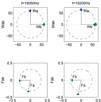
We now control Wa and Wb to obtain a traveling wave. We conducted two test runs, each at a different frequency. For the first test run, we have chosen f = 19 050 Hz, which is exactly in the middle between the two modes. For the other one, we have chosen f = 19 200 Hz, a value closer to the mode b, to check whether or not a traveling wave could be obtained. The results for the two frequencies con-ditions are presented in the space-time plane in Fig. 16, and in the rotating reference frame in Fig. 17.
For each test run, the vibration amplitude of each mode is placed on the right axis, and the condition Wa = jWb is fulfilled. The forces Fa and Fb must be adapted to obtain this condition. For f = 19 050 Hz, this condition results in two modal forces with almost the same amplitude, and phase shifted by approximately π/2, leading to Fa jFb.
We can note here that this does not lead to F1 = jF2
necessarily; indeed, we obtained for this run F1 = −0.23
+ 0.18j and F2 = 0.15 + 0.14j. This is due to the matrix
Kab−1, which combines the two modal forces to obtain the
forces to apply on the beam. Hence, the forces to apply on the beam to obtain a traveling wave depend on the loca-tion of the exciters, which modifies Kab. This conclusion is found to be consistent with [10].
For f = 19 200 Hz, the operating point is closer to mode b, and farther to mode a. The two modal forces Fa and Fb
must adapt to these new conditions: Fa must increase be-cause the participation of the mode a decreases for fre-quencies above its eigenfrequency, as shown in Fig. 4. This is automatically obtained thanks to the control of Wab. consequently, with this method, the control automatically adapts the two exciters’ supply to obtain the traveling wave, through a closed-loop control which responds in 250 ms.
We then measured the deflection at several positions on the beam to estimate the sWr. Measurements were carried out over 30 cm in the middle of the beam, and a spline interpolation was made between the measurements. The results are presented in Fig. 18.
Hence, the traveling wave is not perfect, despite the condition Wa = jWb. To decompose the motion into the traveling and standing components, [15] proposes to fit the measured complex amplitude by an ellipse. With this method, we found sWr = 1.27 at f = 19 050 Hz and sWr = 1.30 at f = 19 200 Hz. a perfect traveling wave would result in sWr = 1.0. These higher values obtained in our case can be due to several reasons.
For instance, the condition Wa = jWb could be badly set, but Fig. 17 shows that is not the case thanks to the control loop.
still, the values of Wa and Wb could be badly estimated in our test bench. In this case, although the control per-Fig. 15. Transient response to step variation of Wbdref from 10 nm to
50 nm.
forms correctly in the rotating frame, a steady-state error would remain in the fixed frame. another explanation is that, for this operating point, the modes higher than mode b may have a negative influence on the sWr. However, we note that the sWr is not improved, nor increased when changing the frequency. Indeed, changing the frequency also changes the repartition of the modes above b.
In this paper, we settle for the values of sWr experi-mentally found, and we do not try to obtain a better sWr, which would lead us to modify the position of the exciters, as shown in [9] and [10]. We note, however, that despite the change in frequency, the sWr of the traveling wave is found to be almost constant for the two runs. Hence, the method allows a traveling wave to be obtained at different frequency conditions, as shown in Fig. 16, which presents the deflection measured with a laser interferometer as a function of time and the position. The two figures are very similar.
We have presented our results on steady-state opera-tions, and we have shown that the control can adapt to different conditions of frequency without changing the sWr. The next section of the paper deals with the tran-sient response of the control.
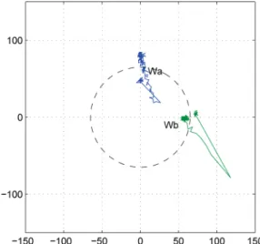
D. Direction Change of the Traveling Wave
opposite direction of the traveling wave can be ob-tained by setting an opposite value for Waref or Wbref. This is experimentally checked and presented in Fig. 19, when Wbdref = −Wbdref.
This figure shows the transient response time; we can observe that a direction reversal is obtained in 150 ms. We also show the trajectory in the rotating reference frame of the vectors Wa and Wb;Wa is not affected by the direction change, because only Wbref is reversed. Moreover, at the
end of the direction change, the two vectors are in quadra-ture.
Fig. 17. diagram in the rotating reference frame of the vibration ampli-tude and the forces for two frequency conditions.
Fig. 18. (a) deflection as a function of space and for 15 different instants (interpolated) (b) complex deflection and the fitted ellipses; stars represent the actual measurements.
E. Frequency Change of the Traveling Wave
In this test run, we test whether the method is ro-bust regarding frequency changes. For that purpose, at t = 0.05 s, the frequency of the traveling wave is changed from f = 18 500 Hz to f = 19 500 Hz. The results presented in Figs. 20 and 21 show no unstable behavior: the defor-mation amplitude of modes a and b return to their refer-ence values after the perturbation. Mode b is clearly more sensitive to this perturbation. This may be due to the fact that in this run, the frequency reaches a value which is very close to the resonant frequency of mode b: the modal forces must adapt accordingly.
V. conclusion
This paper presents a vector control of two vibration modes to obtain a traveling wave in the middle of a
rect-angular beam. For that purpose, a specific model in a rotating reference frame is established. In this reference frame, the vibration amplitudes of the two modes are rep-resented by vectors whose magnitudes are the vibration amplitudes, and the angular position is the associated phase. a validation of this model was proposed by com-parison with experimental runs.
Then, a control based on this model was presented. It was used to control the magnitude and the phase of the vibration amplitude of the two modes to obtain the travel-ing wave. We obtained an sWr of 1.3 for two frequency conditions. This result was obtained over 31 cm in the middle of the beam, corresponding to approximately 66% of the total length. dynamic responses to direction change or frequency change were also presented. The advantage of the method is that it doesn’t need an optimization loop to tune the excitation parameters of the actuators, which leads to a dynamic behavior.
This result was obtained by controlling two modes only, which are measured in the middle of the beam, where the higher modes have less influence. on one hand, this clearly changes compared with some authors’ conclusions, which advise optimization of the participation of up to ten modes. on other the hand, we measured the same sWr for two frequencies, and then with other participation of the higher modes, showing that for the studied beam, these higher modes don’t have a strong influence. This is why we think that the proposed method can produce a traveling wave on other beams, but with non-optimized sWr. Further work should clarify this point.
appendix a
The Experimental Test Bench
The experimental verification was carried out using the experimental test bench of Fig. 22. The constitutive ele-ments of the test bench are shown in Fig. 23. The beam used in this experiment is a 6 × 6 mm square beam with Fig. 19. direction change of the traveling wave at t = 0.02 s.
Fig. 20. Transient response of the vibration amplitude to a frequency change f = 18 500 Hz to f = 19 500 Hz.
Fig. 21. response of the system in the rotating reference frame to a fre-quency change from f = 18 500 Hz to f = 19 500 Hz.
L = 493 mm. Two piezoelectric actuators are used to ex-cite the beam. We used two multistack actuators (cMaP, noliac, Kvistgaard, denmark). These actuators have a low rated voltage (about 30 V) and a resonating frequency well above our working frequency (700 kHz). Thus, we consider that the forces F1 and F2 are directly propor-tional to the supply voltages applied to the piezoelectric actuators named V1 and V2. The actuators are clamped
on the beam by using two specific clamps. The actuators are supplied by two linear amplifiers.
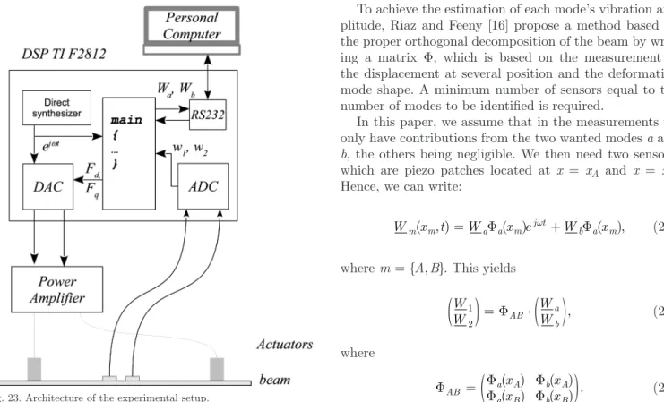
a dsP f2812 (Texas Instruments Inc., dallas, TX) equipped with a digital-to-analog converter produces the voltage references to the amplifiers. In the dsP, a direct frequency synthesizer is running, and produces two signals proportional to r(t) = cos (ωt) and i(t) = sin (ωt). These two signals are then multiplied by the real and imaginary parts, respectively, of F1. The same computation is also achieved for F2. Hence, it is possible to not only synchro-nize the forces F1 and F2, but we can also impose their real and imaginary parts.
We also measure the deformation amplitude at specific points xA and xB with piezoelectric patches bonded on the beam. These patches are used as sensors because the volt-age they produce is directly proportional to w(x, t). The analog-to-digital conversion is synchronized on the signals r and i of the synthesizer. This way, we can measure the real and imaginary parts of these signals. a method de-tailed in the next section is used to deduce Wa and Wb
from these measurements.
Fig. 23 presents an overview of the experimental setup. Finally, a control GUI made using Matlab (The Math-Works Inc., natick, Ma) was created to easily control the parameters of the dsP. a laser interferometer is used to identify the deformation along the whole beam.
appendix B
Identification of Wa and Wb
To achieve the estimation of each mode’s vibration am-plitude, riaz and Feeny [16] propose a method based on the proper orthogonal decomposition of the beam by writ-ing a matrix Φ, which is based on the measurement of the displacement at several position and the deformation mode shape. a minimum number of sensors equal to the number of modes to be identified is required.
In this paper, we assume that in the measurements we only have contributions from the two wanted modes a and b, the others being negligible. We then need two sensors, which are piezo patches located at x = xA and x = xB. Hence, we can write:
W x tm m Wa a mx ej t W x
b a m
( , ) = Φ ( ) ω + Φ ( ), (20)
where m = {A, B}. This yields
W W AB WWa b 1 2 =
( )
Φ ⋅( )
, (21) where Φ Φ Φ Φ Φ AB a A b A a B b B x x x x =(
( )( ) ( )( ))
. (22) Fig. 22. Experimental test bench showing the studied beam, the excitersand the voltage amplifier.
We then choose to place the sensors in positions such that ΦAB is nonsingular. Then, it is possible to calculate the
two contributions of each mode, by
W
Wab AB WW
( )
= −1 ⋅( )
1 2Φ . (23)
Hence, the identification of Wa and Wb can be obtained from the measurements of the deformations at xA and xB
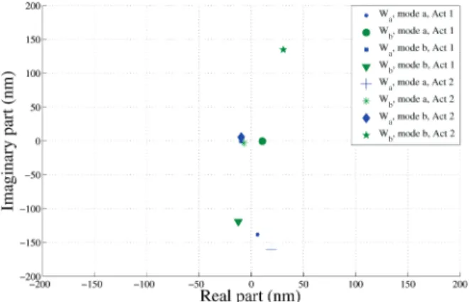
given the deformation mode shapes Φ(x) at each position. In Fig. 24, we present the results of the estimation. For that test, we choose two working frequencies to obtain modes a and b successively. We also chose to supply actua-tor 1 or 2 independently.
From this figure, we can see that when we supply the actuators at the resonance of mode a, then we have Wb
which is very small compared with Wa and vice versa. Moreover, when we compare the cases where F2 = 0 to the cases where F1 = 0, we obtain two results symmetrical for
Wb, while they are almost concentrated for Wa. This is due to the fact that mode a is a symmetric mode, and thus Φa(x1) = Φa(x2) (because we chose x2 = L − x1), and thus Ka1 = Ka2, whereas mode b is antisymmetric, leading to
Kb1 = −Kb2. The results found are thus consistent with
the theory, and we have a way to identify the deformation amplitude for each mode.
references
[1] s. Ueha, y. Tomikawa, M. Kurosawa, and n. nakamura, Ultrasonic
Motors: Theory and Applications. oxford, UK: clarendon Press,
1993.
[2] B.-G. loh and P. I. ro “an object transport system using flexural ultrasonic progressive waves generated by two-mode excitation,”
IEEE Trans. Ultrason. Ferroelectr. Freq. Control, vol. 47, no. 4, pp.
994–999, 2000.
[3] X. li, y. sun, c. chen, and c. Zhao, “oscillation propagating in non-contact linear piezoelectric ultrasonic levitation transporting system—From solid state to fluid media,” IEEE Trans. Ultrason.
Ferroelectr. Freq. Control, vol. 57, no. 4, pp. 951–956, 2010.
[4] s. Miyazaki, T. Kawai, and M. araragi, “a piezo-electric pump driven by a flexural progressive wave,” in Proc. IEEE Micro Electro
Mechanical Systems, 1991, pp. 283–288.
[5] d. sun, s. Wang, s. Hata, J. sakurai, and a. shimokohbe, “Theo-retical and experimental investigation of traveling wave propagation on a several- millimeter-long cylindrical pipe driven by piezoelectric ceramic tubes,” IEEE Trans. Ultrason. Ferroelectr. Freq. Control, vol. 57, no. 7, pp. 1600–1611, 2010.
[6] M. Kuribayashi, “Excitation conditions of flexural traveling waves for a reversible ultrasonic linear motor,” J. Acoust. Soc. Am., vol. 77, no. 4, pp. 1431–1435, 1985.
[7] n. Tanaka and y. Kikushima, “active wave control of a flexible beam: Proposition of the active sink method,” JSME Int. J. 3, vol. 34, no. 2, pp. 159–167, Jun. 1991.
[8] r. Gabai and I. Bucher “spatial and temporal excitation to generate traveling waves in structures,” J. Appl. Mech., vol. 77, no. 2, art. no. 021010, dec. 2010.
[9] B. dehez, c. Vloebergh, and F. labrique, “study and optimization of traveling wave generation in finite-length beams,” Math. Comput.
Simul., vol. 81, no. 2, pp. 290–301, oct. 2010.
[10] a. Minikes, r. Gabay, J. Bucher, and M. Feldman, “on the sensing and tuning of progressive structural vibration waves,” IEEE Trans.
Ultrason. Ferroelectr. Freq. Control, vol. 52, no. 9, pp. 1565–1576,
sep. 2005.
[11] r. Gabai and I. Bucher “Excitation and sensing of multiple vibrat-ing travelvibrat-ing waves in one-dimensional structures,” J. Sound Vibrat., vol. 319, no. 1–2, pp. 406–425, 2009.
[12] M. abu-Hilal, “Forced vibration of Euler–Bernoulli beams by means of dynamic Green functions,” J. Sound Vibrat., vol. 267, no. 2, pp. 191–207, oct. 2003.
[13] c. Giraud-audine and B. nogarède, “analytical modelling of trav-elling-wave piezomotor stators using a variational approach,” Eur.
Phys. J. AP, vol. 6, no. 1, pp. 71–79, 1999.
[14] F. Giraud and B. semail, “a torque estimator for a traveling wave ultrasonic motor—application to an active claw,” IEEE Trans.
Ul-trason. Ferroelectr. Freq. Control, vol. 53, no. 8, pp. 1468–1477, 2006.
[15] I. Bucher, “Estimating the ratio between travelling and standing vibration waves under non-stationary conditions,” J. Sound Vibrat., vol. 270, no. 1–2, pp. 341–359, 2004.
[16] M. s. riaz and B. F. Feeny, “Proper orthogonal modes of a beam sensed with strain gages,” J. Vib. Acoust., vol. 125, no. 1, pp. 129– 131, Jan. 2003.
Frédéric Giraud received the B.s. degree in
1995 from Paris-XI University, graduated from the Ecole normale supérieure de cachan, France in 1996 in electrical engineering, and received the M.s. degree in 1997 from the Institut national Polytechnique de Toulouse and the Ph.d. degree in 2002 from the University lille 1. He is a mem-ber of the electrical engineering and power elec-tronics laboratory of lille, where he works as an associate Professor. His research deals with the modeling and control of piezoelectric actuators.
Christophe Giraud-Audine received his M.
Eng. degree in mechanical engineering from the École nationale supérieure d’arts et Métiers in 1992 and his Ph.d. degree in electrical engineering from the Institut national Polytechnique de Tou-louse in 1998. after two years spent as a research associate at the University of sheffield, he took an associate Professor position at the École natio-nale supérieure d’arts et Métiers. His current re-search focuses on the modeling and control of de-vices based on piezoelectric and shape memory alloys.
Fig. 24. Identification of Wa and Wb for several working conditions, in the complex plane; each point represents the mean values calculated over 100 measurements.
Michel Amberg has been teaching electronics at
the University of lille, France. He graduated from the Ecole normale supérieure de cachan, France in 1981. He has tutored more than a hundred bachelor’s students during their projects in the field of telecommunications, computer science, and electronics. He is now a research engineer at IrcIca, and works on the electronic design of tactile devices.
Betty Lemaire-Semail received the Ph.d.
de-gree in 1990 from the University of Paris XI, or-say. From 1990 to 1998, she was an assistant pro-fessor at the Ecole centrale of lille and she is now a professor at the University lille 1. she is a mem-ber of the electrical engineering and power elec-tronics laboratory of lille and head of the research axis on the control of electrical systems. she has studied electromagnetic motors, and her main field of interest now deals with the modeling and control of piezoelectric actuators for positioning and force feedback applications.