Science Arts & Métiers (SAM)
is an open access repository that collects the work of Arts et Métiers Institute of
Technology researchers and makes it freely available over the web where possible.
This is an author-deposited version published in: https://sam.ensam.eu Handle ID: .http://hdl.handle.net/10985/8898
To cite this version :
Philippe LORONG, Gérard COFFIGNAL, Etienne BALMES, Mikhail GUSKOV, Anthony TEXIER -Simulation of a finishing operation : milling of a turbine blade and influence of damping - In: Proceedings of ASME 2012 11th Biennal Conference on Engineering Systems design and analysis ESDA 2012 July 2-4, 2012, Nantes, France, France, 2012-06-02 - Proceedings of the ASME 11th Biennial Conference on Engineering Systems Design and Analysis--2012 - 2012
Any correspondence concerning this service should be sent to the repository Administrator : archiveouverte@ensam.eu
SIMULATION OF A FINISHING OPERATION : MILLING OF A TURBINE BLADE AND
INFLUENCE OF DAMPING
Philippe Lorong∗
PIMM Laboratory Arts et Metiers ParisTech 151 boulevard de l’Hopital 75013 Paris, FRANCE Email: philippe.lorong@ensam.eu Gerard Coffignal Etienne Balmes Mikhail Guskov PIMM Laboratory Arts et Metiers ParisTech 151 boulevard de l’Hopital
75013 Paris, FRANCE Email: gerard.coffignal@ensam.eu
Anthony Texier
SNECMA, SAFRAN rue H.A. Desbrures BP81, 91003 Evry, FRANCE
ABSTRACT
Milling is used to create very complex geometries and thin parts, such as turbine blades. Irreversible geometric defects may appear during finishing operations when a high surface quality is expected. Relative vibrations between the tool and the workpiece must be as small as possible, while tool/workpiece interactions can be highly non-linear. A general virtual machining approach is presented and illustrated. It takes into account the relative motion and vibrations of the tool and the workpiece. Both de-formations of the tool and the workpiece are taken into account. This allows predictive simulations in the time domain. As an ex-ample the effect of damping on the behavior during machining of one of the 56 blades of a turbine disk is analysed in order to illustrate the approach potential.
NOMENCLATURE
FE Finite Element, τ , t time,
[t,t + ∆t] time interval (current increment), aT entity related to the Tool,
aW entity related to the Workpiece,
a(i) entity related to the elementary tool T(i), ~a vector, 3D usual physical space,
∗Address all correspondence to this author.
Rs coordinate system s (and frame),
{A}s column of components (or coordinates) inRs, [A]s matrix (components inRs),
~
Ω angular velocity vector with respect toRa, [M] mass matrix,
[D] damping matrix, [K] stiffness matrix, [G(~Ω)] Coriolis matrix,
[N(~Ω)] centrifugal acceleration matrix, [ ˜D(~Ω)] = [D] + [G(~Ω)]
[ ˜K(~Ω)] = [K] +12[ ˙G(~Ω)] + [N(~Ω)]
[H(X )] value of the FE displacement interpolation matrix at point X in the mesh,
columns of generalized:
{q} unknown displacements (do f ) { ˙q} unknown velocities
{ ¨q} unknown accelerations {δ q} virtual displacements, {Q} known (given) forces,
{Q}W/T cutting forces acting on the tool, {Q}T/W cutting forces acting on the workpiece.
INTRODUCTION
Milling allows to get very complex geometries and thin parts, such as turbine blades. These parts, that are obtained by means of multi-axis machining and numerical control (NC) and may be very costly. In this context, numerical simulations can have a central role when dealing with the optimisation of the machining conditions because iterative experimental approaches based on trial and corrections quickly reach their limits. This results from the wide range of cutting conditions encountered along the tool trajectories which can add irreversible geometric defects on the part. This is particularly true for finishing opera-tions when a high surface quality is expected. Relative vibraopera-tions between the tool and the workpiece must be as small as possible, while tool/workpiece interactions can be highly non-linear.
Today, numerical simulation of machining processes have not yet reached the maturity that can be observed in the simula-tion of other manufacturing processes. Our approach [1], which is applied to the virtual machining of a finishing operation in milling, aims to be a general one.
By ”virtual machining” we mean the numerical process al-lowing to simulate and verify the pertinence of tool paths, taking into account vibrations and material removal in an integrated and general approach. The final description of the surface geometry at the end of the simulation is one of the aims of the simulation, but it is not the only one. Checking the stability, the level of vi-brations and the possibility to reduce them by means of adapted modifications of the part boundary conditions, tool paths and of the spindle angular velocity are also among the goals.
Several models have to be set up and coupled to reach this target. To build a predictive model of the dynamics it is neces-sary to get the instantaneous thickness h of the ”boolean chip” (Fig. 1b), which is associated with the simplified model of ma-terial removal (”3D eraser”) which is adopted (Fig. 1a). At the same time a sufficiently accurate description of the interaction between the tool and the workpiece must be achieved. The in-stantaneous thickness h is required along all points of the cut-ting edges. It allows to calculate the forces accut-ting both on tool and workpiece. The forces and resulting vibrations allow then to calculate the evolution of the thickness. This corresponds to a kind of closed loop governing the dynamics of the tool on the one hand, and of the workpiece on the other hand. In order to get both the instantaneous thickness and machined surface, a ge-ometric model which undergoes the same deformations as the workpiece is used. This model, which uses dexels [2], is linked to the finite element model of the workpiece, but is completely different.
In the approach we propose, numerical simulations rely on several models:
1. a numerical model to describe the dynamics of the tool is described section 4.3. As shown section 4, when milling tur-bine blades, the flexibility of the tool softens the dynamics
actual chip at t time t time t+ ∆t actual chip at t+∆t virtual workpiece virtual workpiece actual workpiece actual workpiece
virtual machining actual machining (a) Material Removal inRm
swept domain from t to t+∆t boolean chip in interval t to t+∆t h rake faceΣc (i) cutting edgeΓc (i) elementary tool T(i) t
t+∆ t
t+∆ t/2
(b) Swept domain inRmand boolean chip
FIGURE 1: MATERIAL REMOVAL AND BOOLEAN CHIP (2D ILLUSTRATION).
of the whole system and must be taken into account because it has a significant influence on the stability limit;
2. a numerical model to describe the dynamics of the work-piece which allows to compute its vibrations, and thus its deformations, during all the machining operation. It is de-scribed section 1.2;
3. models for the interaction between the tool and the work-piece. They allow the calculation of the forces applied by the tool to the workpiece, by means of functions of the instan-taneous ”cut section” Σ along Γ, the set of all active cutting edges. They are presented section 2.
4. a model of the geometry of the machined surface of the workpiece. This model, which is updated at each time step to follow the material removal, allows to calculate anywhere the cut section Σ and an associated depth of cut h. It gives the description of the surface geometry at the end of the sim-ulation (and at any time step). When the dynamic stiffness of the workpiece is of the same order or less than that of the tool in the considered frequency range of force variations, it should be noted that in order to get an accurate value for h it is absolutely necessary to take into account the deforma-tions of the workpiece. This is particularly true for finishing
rake face Σc(t) cutting edgeΓc cut surfaceΣ Σ Γ elementary tools (a) (b) (c) zoom Σc Γc
FIGURE 2: END MILL : RAKE FACE ΣcOF ONE OF THE TEETH AND CUTTING EDGE Γc. SURFACE Σ, ACTIVE
CUTTING EDGE Γ AND ELEMENTARY TOOLS.
operations. The model of the geometry must thus follow the workpiece deformations.
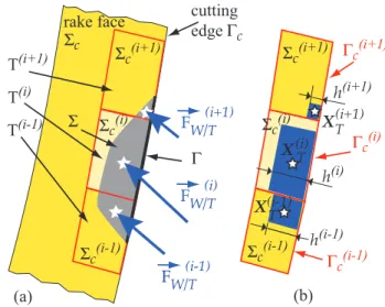
The original and important point in our approach to virtual machining, is that it takes into account both instantaneous defor-mations (vibrations) of the tool and the workpiece in the simula-tion when determining the local depth of cut h and the material removal. As a matter of fact, to get h, which can also be seen as the thickness of a ”boolean chip” (see Fig. 1b) all along the set Γ of all active cutting edges at time t, we need a good descrip-tion of the subset Σ of the rake face Σcwhich contains Γ and has generated the boolean chip.
Figure 2 illustrates for one of the teeth of an helicoidal end mill the subsets of Σc, Γc, Γ and Σ for that tooth.
The decomposition of the tool in elementary tools (Fig. 2-c, Fig. 3-a and Fig. 3-b) allows a versatile description of its geometry and provides an efficient means to compute both h(i) and the material removal.
Examples of the results that can be obtained are shown for a turbine blade section 4: surface defects (waviness and shape), values of limit damping and amplitude of vibrations during ma-chining. An example taking into account the whole turbine disk with its 56 blades is given 4.4.
Results shown section 4 have been obtained using Nessy, a research software developed at PIMM, Arts et Metiers ParisTech.
1 OUTLINE OF THE NUMERICAL APPROACH
The final aim of our approach is to set up a model for virtual machining in a systematic way, as versatile as finite elements are today. (a) Γ Σ FW/T (i+1) F W/T (i) F W/T (i-1)
rake face cutting
edge Γc h(i) h(i+1) h(i-1) (b) Γc (i) Γc (i-1) Γc (i+1) Σc (i+1) Σc (i-1) Σc (i) Σc (i+1) Σc (i-1) Σc (i) Σc T(i+1) T(i) T(i-1) XT (i+1) XT (i) XT (i-1)
FIGURE 3: ELEMENTARY TOOLS: ACTING FORCES, T(i), Σ(i)c AND CUTTING DEPTH h(i), CLOSE-UP FROM Fig. 2.
Unlike other recent works dealing either with the flexibil-ity of the workpiece and related forces, vibrations and stabilflexibil-ity ( [3, 4]) or with the simulation of the whole machining process in order to check the final surface on purely geometric considera-tions simulating the whole envelope of the tool trajectory ( [5,6]), we blend both approaches and manage any geometry of work-piece and tool in a unique simulation.
Here, the ”tool” takes a general sense and must be under-stood either as a one piece tool or as a set of inserts, including drills, cutters and end mills, or as a small element of a tool near one of its cutting edge. This element of a drill, a cutter, an insert, is called an ”elementary tool” Fig. 2-c and Fig. 3-a.
Once FE models have been built, the general system of equations to be solved , can be written [7] for the tool T and workpiece W :
[M]T.{ ¨q}T+ [ ˜D]T.{ ˙q}T+ [ ˜K]T.{q}T = {Q}T+ {Q}W/T (1) [M]W.{ ¨q}W+ [ ˜D]W.{ ˙q}W+ [ ˜K]W.{q}W = {Q}W+ {Q}T/W (2)
{Q}T and {Q}W take eventually into account known acting forces.
{Q}W/T and {Q}T/W are determined by Eqn. (4) and Eqn. (6) and necessitate a good description of the boolean chip instan-taneous thickness. These generalized forces play a major role in the approach and depend upon the accuracy of the models de-scribed sections 2 and 3.
In Eqn. (1) and Eqn. (2) the dofs are defined in local coordi-nate systems (and frames)RT andRW. Both are in motion, with large translations and rotations, in the inertial frame and one of
its coordinate systemsRa. Thus, terms in Eqn. (1) and Eqn. (2) are not defined in the same system of coordinates.
In the general case {q}T are defined in a rotating frameRT undergoing large rotations, to describe with respect to it the small translations and rotations of the tool. The same is done for {q}W to describe the workpiece in small translations and rotations in its related frameRW.
~
ΩT and ~ΩW are the angular velocities ofRT andRW with respect toRa. When ~Ω =~0 for a frame, simplifications appear. In this case, this leads for the frame, in Eqn. (1) or Eqn. (2), to [ ˜D] = [D] and [ ˜K] = [K].
Let ~fT/W be the surface density of forces exerted on the workpiece by the tool. This occurs all along Γ, on the set Σ of surfaces adjacent to the cutting edges Γcwhich are in contact with the workpiece.
The effect of ~fT/W = −~fW/T is approximated by means of a model described section 2. It allows to approximate ~fT/W by a set of nf discrete forces ~F(i)T/W acting on the workpiece at points XW(i).
As a matter of fact, each force ~F(i)T/W has a companion ~
FW(i)/T= −~F(i)T/W acting on the tool at point X(i)T (action and reac-tion). The two points X(i)T and XW(i)are located at the same point X(i)a ofRa, at time τ.
Once the set of (~F(i)W/T, ~F(i)T/W) pairs and related (X(i)T , XW(i)) pairs are known, they are projected in their respective coordi-nate systems inRT andRW leading to ({F}(i)W/T, {F}(i)T/W) and ({X }(i)T , {X }(i)W). The virtual displacement {δ u}(i)T at point X(i)T of the tool is given by Eqn. (3) and {Q}W/T is then obtained by means of the finite element formulation given by Eqn. (4):
{δ u}(i)T = [H(X(i)T )]T . {δ q}T (3) {Q}W/T = nf
∑
i=1 [H(X(i)T )]TT . {F}(i)W/T (4)Similar relations hold for the workpiece:
{δ u}(i)W = [H(X(i)W)]W . {δ q}W (5) {Q}T/W = nf
∑
i=1 [H(X(i)W)]WT . {F}(i) T/W (6)Very often the FE model of the workpiece leads to a large number of dofs in {q(t)}W. In order to be efficient, a reduction ( [7]) must be done. This is not discussed here, but it is done and leads to a smaller set of dofs {q0}
W. This can also be nec-essary for the tool. Such reductions lead to {q}k= [R0]k. {q0}k
and {δ q}k = [R0]k. {δ q0}kwhere [R0]kis the reduction matrix. The index k represents T or W . In the lhs of Eqn. (1) and Eqn. (2) the {q}k are changed in {q0}k, the matrices are pre and post multiplied by [R0]Tk and [R0]k and the rhs are premultiplied by [R0]Tk. Usually a reduction using the first modes of the FE model is done. Static deformations can by added.
1.1 Tool Dynamics
A FE model is set up for the tool in its associated coordinate systemRT. In most situations, a sufficient accuracy is obtained by means of an assembly of beam elements and rigid bodies. In any case this leads to an approximation of the displacement in the form:
{u(X, τ)}T = [H(X )]T . {q(τ)}T (7)
By means of Eqn. (3) and Eqn. (7), the virtual work principle leads to Eqn. (1) ( [7]).
Then, the FE solution is obtained step by step for τ ∈ [0,tF], at time steps t0= 0, t1= ∆t, t2= 2∆t, t3= 3∆t, · · · ,t, t + ∆t, · · · by means of a finite difference scheme using for instance the Newmark method ( [7]).
1.2 Workpiece Dynamics
A FE model is set up for the workpiece in its associated coordinate systemRW and, as for the tool, leads to Eqn. (2).
In order to make easier the modeling of virtual material removal, which is described section 2, ten nodes tetrahedral isoparametric elements are prefered. The FE approximation of the displacement is given by Eqn. (8):
{u(X, τ)}W = [H(X )]W . {q(τ)}W (8)
The step by step approach of section 4.3 is used, with the same time steps and increment ∆t.
1.3 Iterations
As stated before, Eqn. (1) and Eqn. (2) are not independent because {Q(τ)}T and {Q(τ)}W are — at least — functions of the h(i)which are themselves functions of the relative evolution inRaof the displacements ~ua(X , τ)T of the tool and ~ua(X , τ)W of the workpiece for τ ∈ [t,t + ∆t] near the domain swept by all Σ(i)c . They are thus functions of {q(τ)}Tand {q(τ)}Win this time interval. If a linear variation of these generalized displacements is assumed with respect to τ, {Q(τ)}Tand {Q(τ)}Wonly depend upon {q(t + ∆t)}T and {q(t + ∆t)}W which are the unknown at time t. In addition to the step by step solution, we thus need iterations to satisfy both Eqn. (1) and Eqn. (2) at the end of the time interval [t,t + ∆t].
2 MATERIAL REMOVAL
This model is necessary to get an accurate coupling between Eqn. (1) and Eqn. (2) by means of {Q}W/Tand {Q}T/W i.e. find-ing at time t + ∆t both the opposite forces ~F(i)W/T and ~F(i)T/W and the points X(i)T and X(i)W, where they are acting on the tool and on the workpiece. These points are coincident inRaat t + ∆t.
An example of the pair ~FW(i)/Tand X(i)T is given Fig. 3-a. In our approach, the usual concept of boolean operations is used to simulate, at a macroscopic level, the material removal. The action of each elementary tool is simply modelled as if it was a ”3D eraser of matter” as illustrated (in 2D) Fig. 1a and Fig. 1b. This is what is done in stability analysis and is in good agreement with experiments ( [3, 4]). This assumption is also made for the whole and a priori envelope of the tool along its paths in geometric virtual machining ( [5, 6]).
We make this assumption for each time interval [t,t + ∆t], thus following each elementary tool T(i) and its rake face Σ(i)c during its motion, which is not the case when only the envelope of the whole rotating tool is considered. Here, an accurate sim-ulation of the material removal history cannot be avoided, time step by time step, to reach our goals.
2.1 Material Coordinates
We have to face the difficulty that both the tool and work-piece undergo motion and deformation. In this context, we must consider a material coordinates system Rm associated to the workpiece. It is associated to the undeformed initial geometry of the workpiece. InRmthe workpiece remains a rigid body at rest, if we except the material removal which decreases its vol-ume.
The boolean operation between the volume swept during the time step by Σ(i)c and the workpiece domain, inRmdefines the boolean chip which makes the matter of the workpiece be re-moved from the geometric model of the workpiece as shown Fig. 1b. This allows to calculate values of h(i)in each elementary rake face Σ(i)c and the related positions {X }(i)T . h(i)is a local average of the depth of cut along Γ(i)(and during ∆t) as illustrated Fig. 3-b and Fig. 1b. This value is used to feed the model to get the ~
F(i)T/W.
2.2 Swept Domains
To describe the swept domain, it is necessary to set up a systematic and efficient way to model its geometry inRW during the interval [t,t + ∆t]. This must be done several times in [t,t + ∆t], due to iterations to satisfy both Eqn. (1) and Eqn. (2).
A mesh pattern is associated to each rake face Σ(i)c . This pattern is shown Fig. 4 in the case of a middle added section. Plane triangles are chosen. The coordinates of their 3 vertices
positions of the rake face Σc (i)of T(i) t Γc (i)cutting edge of T(i) at time t t+ ∆t/2 t+ ∆t t t+ ∆t/2 t+∆t
FIGURE 4: SWEPT DOMAIN INRmBY THE RAKE FACE Σ(i)c OF AN ELEMENTARY TOOL T(i): MESH PATTERN.
are deduced from the positions at t and t + ∆t of Σ(i)c as given by {q}T and by the positions ofRTandRW inRa. The knowledge of the coordinates of its 4 vertices defines the position of Σ(i)c .
Intermediate positions of Σ(i)c (at t + ∆t/2 for instance, or more) may be used to take into account the rotation due to the relative motion ofRT with respect toRW.
Once the coordinates of the vertices have been obtained, they are changed to coordinates inRW to prepare the obtention of the boolean chip. This thus gives the positions of all the ver-tices of the mesh (one a t, one at t + ∆t, and if the chosen pattern needs intermediate values, position at intermediate times).
2.3 Interaction Forces
An efficient model to get ~F(i)T/W the forces applied to the workpiece by the tool must be chosen. Any representative model can be used. At least it must allow to determine the ~F(i)W/T on each Σ(i)c by means of h(i)and b(i):
~
F(i)W/T = ~F(i) W/T(h
(i), b(i), · · · ) (9)
b(i)is determined such that the local cut section for T(i) is the product h(i)b(i). Other parameters may be added. The decompo-sition of the tool in nf T(i)elementary tools allows very flexible modeling. Kienzle’s model [8] or more advanced models such the one developed in [9] are good candidates. The latter is used in this paper and for the tool-blade pair shown section 4 the model is the one given p.117 of [10].
3 GEOMETRIC MODEL OF THE MACHINED SURFACE
A recent overview of geometric models in the context of vir-tual machining can be found in [4]. In our case the geometric model of the machined surface must be updated at each time step to follow the material removal, which is not usually the case. The model must allow to calculate h(i)in any elementary tool T(i)in order to get the distribution and values of the forces applied by
FIGURE 5: MACHINED SURFACE RECONSTRUCTED FROM DEXELS (ZOOM ON A FRACTION OF THE
SURFACE SHOWN Fig. 13.
the tool to the workpiece. It gives the final description of the sur-face geometry at the end of the simulation, and its evolution time step by time step from the beginning of the simulation.
As explained in previous sections, in order to get an accu-rate value for h(i), it is absolutely necessary to take into account the deformations of the workpiece and its relative motion with re-spect to the tool. This is particularly true for finishing operations. The model of the geometry must thus follow these deformations. In the current state of our work, the geometric model of the workpiece uses dexels to model the domain of the workpiece and its boundary. This allows a robust and efficient calculation of all boolean operations. An illustration of the refinement that we use in the simulation of an industrial part to describe the geometry of the machined is given Fig. 5. The boundary of the workpiece domain (the machined surface) is reconstructed from the dexels in order to give a smooth representation. Each small quadrilateral face represents the trace of one dexel (nearly perpendicular to the surface in this particular case). Figure 5 gives a close-up of a small zone of the blade surface. This model is linked to the FE one by means of a mapping Φ which is illustrated Fig. 6.
Dexels are set up inRm. Dexels are implicitely linked to the finite elements of the workpiece and to its deformation and mo-tion by means of Φ. By means of its inverse Φ−1the coordinates of the vertices necessary to build the domain swept by the rake face Σ(i)c are brought back fromRW toRm and thus takes into account all relative motions of the tool with respect to the matter.
3.1 Mapping FromRmToRW
It must be kept in mind that during the time interval [t,t + ∆t], the deformation of the workpiece changes as well as the one of the tool. A relative rigid body motion exists also betweenRT andRW and combines with the deformation. This is the reason
Om material frame R
m
dexels rakeface
time t +∆t time t (a) (c) (a) (b) (b) (d) Φ(t + ∆t) Φ(t) material frame Rm Om t + ∆t t + ∆ t/2 t dexels OW frame RW rake face rake face OW frame RW rake face
FIGURE 6: DEXELS AND MAPPINGS Φ(t) AND Φ(t + ∆t) FROMRmTORW (2D ILLUSTRATION).
why we use the usual material coordinate system. This coor-dinate system may be seen as a reference frame Rm in which the points of the workpiece are at rest. In this frame the work-piece keeps its undeformed configuration, if we except the mate-rial removal. It must be noted that the definition of the matemate-rial removal can only be defined in such a material frame when de-formation occurs.
The geometric model of the workpiece is thus set up inRm. A mapping Φ(τ) fromRmtoRW is made. If linear isoparametric tetrahedral elements are used, Φ may be explicitely defined by the FE model inside the workpiece. It has to be extended to its outside, as shown Fig. 7a in order to be able to bring, by means of its inverse Φ−1(τ), the swept domain by each Σ(i)c for τ ∈ [t,t + ∆t] inRm. We need that to calculate the material removal during this time interval and then calculate each h(i) and other parameters.
3.2 Mapping Construction
The construction of the mapping Φ is done by means of a finite element mesh of a part of the outside of the workpiece. This extension of the mesh of the workpiece uses tetrahedral elements which are compatible and connected to the workpiece ones via the dofs of the nodes that they share. To simplify, a schematic 2D illustration of such meshes is given Fig. 7b and Fig. 7c. The partial mesh of the outside is used to get the images of the vertices of each rake face Σ(i)by Φ−1(t) and Φ−1(t + ∆t) at time steps t and t + ∆t. Once this is done, the boolean chip can be calculated as well as the forces ~F(i)W/T and ~F(i)T/W.
Mesh of the outside
Mesh of the workpiece OW
(a) Meshes inRm: mesh of the workpiece and of a part of its outside
OW
(b) Initial deformed configuration, after clamping
rake face
Σc
(i)(t)
OW
(c) Current deformed configuration at time t
FIGURE 7: DEFORMED CONFIGURATIONS INRW, OF THE WORKPIECE.
4 EXAMPLE OF A TURBINE BLADE 4.1 General Context
The power of the proposed method is illustrated on an indus-trial workpiece. Investigations had been made, based on experi-mental tests, in order to be able to manufacture the blade shown Fig. 8. We show here the results of simulations that were made by means of our method after completion of these experiments. Due to the industrial conditions of these experiments it was not possible to dispose of any kind of signal record. As a conse-quence, the only available information is:
- an accurate description of the geometries of the end-ball cut-ter, the initial dimensions of the workpiece, the NC descrip-tion of the trajectories of the mill as illustrated Fig. 8; - the mechanical constants (mass density ρ, Young’s modulus
Eand Poisson’s ratio ν) for the workpiece and the tool; - a cutting law extracted from [10] and which was identified in
very similar cutting conditions (tool, workpiece, machining parameters).
So the aim of the simulations was principally to show that the conditions that were found experimentally would have been guided efficiently by means of simulations. We have also tested the ability of the approach to deal with large FE model such as a whole turbine disk.
Rake faces of the tool (end ball mill, helix 30°)
Box of dexels (a) View 1: the blade and, on the right, the positions of the four rake
faces of the end ball mill at the beginning of machining.
Trajectory of point E
E
Cutter axis
(b) View 2: the imposed trajectory of the center point of the cutter end E, inRmand the positions of the four rake faces at τ = 0.
FIGURE 8: VIEWS INRmAT τ = 0 OF THE BLADE, TOOL, TOOL PATH AND DEXEL BOX.
4.2 Main Features of the Simulations
We consider a fraction of the finishing operation of a turbine blade. First it is considered to be alone, then as a part of the whole blisk which has 56 blades.
Figure 8 shows the skin of the FE mesh used to model the dynamics of the blade and the rake faces of the end ball mill. It is a four helical fluted one piece tool (helix angle 30). It is shown at τ = 0, before starting the simulation. Also shown are: the trajectory which is given to the virtual NC control for point E and the edges of the box where are placed the dexels which allow to model the material removal and the related machined surface modifications.
The angular frequency of the cutter is 2700 rev/min. The effects of the rotation of RT are neglected in Eqn. (1) and do not exist in Eqn. (2) (RW does not rotate). The above mentioned reduction technique is used for both the tool and the workpiece. Two mode shapes of the tool are kept to build [R0]T (the first pair of natural bending modes associated with the double natural fre-quency at 1 960 Hz). The ten first mode shapes of the blade (the workpiece) are used to build [R0]W. The corresponding natural frequencies are in the interval [1 130 Hz , 13 140 Hz].
A typical result at the end of a simulation is shown Fig. 9b. Excessive vibrations appeared during this virtual
machin-Studied area subjected to machinin g Area not sudied
(a) Orientation of the blade in subsequent illustrations
zone 1
zone 2
zone 3 zone 4
(b) Typical result of the simulation at any selected time τ. FIGURE 9: MACHINED SURFACE PREDICTED BY
VIRTAL MACHINING: TYPICAL RESULT
ing. Figure 9a shows the orientation of the blade which is kept all along the following figures to illustrate the results.
Surface defects induced by relative vibrations can easily be identified in Fig. 9b. Four zones can be distinguished on the machined area:
- zone 1: excessive vibrations of the blade, the cutter went through the workpiece ! The blade is a thin part in this zone, - zone 2: occurring vibrations tend to be stabilized, (the
mo-tion of the tool is from the left to the right), - zone 3: stable vibrations,
- zone 4: new occurrence of vibrations, the amplitude of which is increasing as the tool gets closer to the end of the zone (edge of the blade).
In this example, unstable zones are thus observed in the areas where the local blade stiffness is the smallest (zones where the blade is the thinnest).
4.3 The Blade Alone : Influence of Damping
As said above we did not dispose of any measurements for the tool or workpiece as mounted during the actual machining. So it was not possible to quantify the actual levels of damping.
This led us to model the damping of the workpiece by means of a unique common modal damping ratio ξW for the 10
consid-(a) Damping ratio ξW= 0.001 (b) Damping ratio ξW= 0.003
(c) Damping ratio ξW= 0.005
FIGURE 10: FLEXIBLE WORKPIECE / RIGID TOOL.
ered modes. The same is done for the two modes of the tool introducing a modal damping ratio denoted ξT. Then, minimum values ¯ξ of the damping ratio, which appear to be limit values in order to get stable conditions are extracted from the simulation.
If we assume that the machining parameters were chosen at SNECMA in order to minimize the duration of the finishing operation, while avoiding the occurrence of defects, they are such that they lead to be near but below the stability limit. The aim of the simulations that are proposed here is to get evaluations of the limit damping ratios, based on the above assumptions. This is done independently for the tool and the workpiece.
First the tool is assumed to be perfectly rigid. Then this assumption is made for the workpiece. Finally, both tool and workpiece vibrations are taken into account.
The resulting geometry of the machined surface is shown Fig. 10 for three values of the damping ratio ξW. In this simula-tion the tool is assumed to be perfectly rigid. The limit damping ratio obtained is near a value of ¯ξW = 0.005. It can be noticed that for this kind of part, this small value is in good agreement with usually observed values.
Figure 11 has been obtained assuming that the workpiece is perfectly rigid. It shows the influence of the damping ratio in-troduced for the tool on the geometry of the computed machined surface. The results are given for three values of ξT. The limit damping ratio obtained is near a value of ¯ξT = 0.03. This value is also a realistic one, since the tool is mounted on a spindle, the design of which tends to increase damping in order to reduce the
(a) Damping ratio ξT= 0.01 (b) Damping ratio ξT= 0.02
(c) Damping ratio ξT= 0.03
FIGURE 11: FLEXIBLE TOOL / RIGID WORKPIECE
vibrations.
To end theses series of simulations, the vibrations of both the tool and the workpiece are taken into account. Fig. 12 shows the different zones that can be observed on the machined surface in this case. An important observation of these simulations is that for damping ratios slightly under the limit observed in the case where either the tool or the workpiece is rigid, for instance (ξW= 0.003, ξT= 0.01) or (ξW= 0.004, ξT = 0.02) the quality of the machined surface is better than the one obtained assuming the workpiece or the tool to be rigid.
From the above example, it seems that both deformations and vibrations of the tool and the workpiece have to be consid-ered to be sure of what is predicted by the model. However, for the simulated operation, the stability limit seems to remain reached for values near ξW = 0.005 and ξT = 0.03).
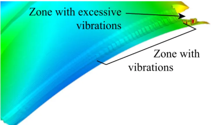
4.4 The Blade and the Whole Turbine Disk
Investigations were done to evaluate the influence of the dy-namics of the disk and its other 55 blades which are neglected when considering the blade alone. Resulting simulated machined surfaces are shown Fig. 13. The modal basis used to build [R0]W contains the first 180 mode shapes. The advantage of the cyclic symmetry of the turbine disk [11, 12] is taken to calculate this
Zone with
vibrations
Zone with
vibrations
(a) (ξW= 0.003, ξT= 0.01)Zone with
vibrations
(b) (ξW= 0.004, ξT= 0.02)Zone with
small vibrations
(c) (ξW= 0.005, ξT= 0.03)FIGURE 12: TOOL AND WORKPIECE BOTH FLEXIBLE, 10+2 MODES.
modal basis. For this virtual machining, the chosen damping ra-tios are the same as those of Fig. 12c (ξW = 0.005, ξT= 0.03).
It can be observed that there exists a zone which is slightly more concerned by vibrations when considering the whole tur-bine disk. Theses results should be compared to instrumented experimental results in order to go further in the analysis.
Never-Zone with
vibrations
Zone with excessive
vibrations
FIGURE 13: TOOL AND WORKPIECE BOTH FLEXIBLE, 180+2 MODES, CYCLIC SYMETRY (ξW = 0.005, ξT = 0.03)
theless it is clear that the quality of the mechanical model of the workpiece is of importance when dealing with the stability of a thin workpiece like the blade under consideration. When taking into account 180 modes, the simulation is twice longer as it is for 10 modes of the blade considered alone.
CONCLUSIONS
In this paper, the main lines of a general method to simu-late any machining operation, in the case where the vibrations and deformations of the workpiece cannot be neglected was pre-sented. It uses a combination of several models in order to set up and solve the equations taking into account the whole dynamics of the pair tool plus workpiece. Associated to reduction methods, complex Finite Element models may be used to accurately take into account the deformations and vibrations of both the tool and the workpiece.
The original core of the method is the efficient construction of a fast mapping which allows to bring the rake faces of the tool into the material frameRm for each iteration of each time increment.
Some of the features of the approach were demonstrated by its application to an industrial workpiece. In order to illustrate the capabilities of the approach, the influence of damping on the stability limit, for a particular area of the blade, was shown by means of the visual observation of the machined surface. More accurate tools can be developed to quantify the defects from the database which describes the virtual machined surface. Once this database exists and contains a reliable machined surface descrip-tion, it can be observed as actual machined surfaces are.
References
[1] Lorong, P., Yvonnet, J., Coffignal, G., and Cohen, S., 2006. “Contribution of computational mechanics in numer-ical simulation of machining and blanking”. Archives of Computational Method in Engineering, 13, pp. 45–90. [2] Van Hook, T., 1986. “Real-time shaded nc milling display”.
In SIGGRAPH’86, pp. 15–35.
[3] Ma˜n´e, I., Gagnol, V., Bouzgarrou, B., and Ray, P., 2008. “Stability-based spindle speed control during flexible work-piece high-speed milling”. Int. J. of Machine Tools and Manufacture, 48, pp. 184–194.
[4] Hong Tzong, Y., and Lee Sen, T., 2009. “Efficient nc sim-ulation for multi-axis solid machining with a universal apt cutter”. J. of Computing and Information Science in Engi-neering, 9.
[5] Lee, S. W., and Nestler, A., 2011. “Complete swept volume generation, part i: Swept volume of a piecewise c1-continuous cutter at five-axis milling via gauss map”. Computer-Aided Design, 43, pp. 427–441.
[6] Lee, S. W., and Nestler, A., 2011. “Complete swept volume generation, part ii: Nc simulation of self-penetration via comprehensive analysis of envelope profiles”. Computer-Aided Design, 43, pp. 442–456.
[7] Gm¨ur, T., 2008. Dynamique des Structures. Analyse modale numrique.Presses Polytechniques et Universitaires Romandes (EPFL).
[8] Kienzle, O., and Victor, H., 1957. “Spezifische schnit-tkrafte bei der metallbearbeitung”. Werkstofftechnik und Machinenbau, 45, pp. 224–225.
[9] Bissey, S., 2005. “D´eveloppement d’un mod`ele d’efforts de coupe applicable `a des familes d’outils : cas du fraisage des aciers trait´es thermiquement.”. PhD Thesis, Arts et Metiers ParisTech (ENSAM), April 2005.
[10] Corduan, N., 2006. “Etude des ph´enom`enes vibratoires en fraisage de finition de plaques minces : application aux aubages de turbines a´eronautiques”. PhD Thesis, Arts et Metiers ParisTech (ENSAM), May 2006.
[11] Sternch¨uss, A. and Balmes, E. and Jean, P. and Lombard, JP., 2009. “Reduction of Multistage disk models : applica-tion to an industrial rotor”. Journal of Engineering for Gas Turbines and Power, 131.
[12] Balmes, E., and Bianchi, J., 2008-2011. http://www.sdtools.com/pdf/rotor.pdfSDT/Rotor, User’s Manual. http://www.sdtools.comSDTools.