1
Université de Montréal
Rapport de recherche
Y a-t-il une relation entre volatilité macroéconomique et croissance économique? Présenté par :
Christopher Lang Afah
Directeur de Recherche : Alessandro Riboni
Département de sciences économiques Faculté des arts et sciences
2 Table of Contents
1. Introduction ………..2
2. Models of Economic Growth………..5
3. Literature Review………..16
4. Data……….17
5. Model……….19
6. Empirical Analysis and Results……….20
7. Concluding Remarks………24 References
3 1. Introduction:
Macroeconomists have mythically in the past regarded business cycles and economic growth as two distinct and unrelated areas of research. This myth has been rejected and knowledge in this relatively new and active area of research has been revolutionized. The real business cycle (RBC) papers of the 80s dominated by Kydland and Prescott (1982), Long and Plosser (1983) which emphasized productivity shocks as the principal source of economic fluctuations have been used as the main bridge in linking macroeconomic trend and cyclicality. The AK approach by Romer (1986) has also been used to bridge the gap between short term fluctuations and long term growth. The Schumpeterian approach named after its founder Schumpeter has been applied by researchers recently to establish the link between macroeconomic volatility and economic growth. This equation is centered on the research arbitrage equations.
To this end, the cyclicality of R&D investments over the business cycle can be accounted for by the following reasons: First, innovations lead to imitation and these innovations are are more profitable during booms. Second, and finally in the absence of credit constraints, during recessions, firms reorganize their structure, reallocate their resources more efficiently and even reinnovate in anticipation of good days (booms). This fact is reechoed by Schumpeter himself: “Recessions are but temporary. They are a means to reconstruct each time the economic system on a more efficient plan”.
Notwithstanding this fact, we know that in the real world context, recessions greatly damage the financial health of many industries and firms. There is clearly an asymmetric between the damage caused by a recession and the benefits of a boom. The credibility of firms/industries to acquire loanable funds becomes undoubtable if not questionable. The Schumpeterian paradigm goes a little further to predict that in less financially
4
developed systems, the causality between macroeconomic volatility and economic growth is strongly negatively correlated. This result is further reiterated by Garey Ramey and Valerie Ramey (1995) paper on cross-country evidence between volatility and economic growth. This substantiates the correlation between credit constraints and financial development and economic growth. The fact that most less financially developed systems limit the ability of firms to acquire credit may account for less economic growth in those systems.
A very important rendition to the link between volatility and economic growth is provided by the stochastic growth model of Acemoglu and Zilibotti (1997). They argue fiercely that due to the fact that most investments involve a start up cost, underdeveloped economies with limited guarantees can just do a only a little. This also means that their ability to diversify, control and avoid idiosyncratic risk is greatly reduced and limited.
There is no definitive causation between volatility and economic growth. The relationship can either be positive or negative. Two serious reasons have been advocated for this.
First, in the presence of credit constraints, long term investments are more riskier to undertake. Most rational (risk averse) investors would shy away from such ventures thereby lowering long term investments over time and this further lowers the growth rate. This also explains the procyclicality of R&D investments under very stringent credit conditions.
Second, a higher volatility in a more credit constrained economy would mean a deeper recession and this means lower investment capabilities of firms. This means that in a recession higher volatility would have a highly negative effect on R&D investments while in booms, the effect would be slightly positive. This accounts for the fact that in credit constrained economies, the relationship between volatility and economic growth is
5
expected to be negative. Examples of empirical studies confirming this finding include Garey Ramey and Valerie Ramey (1995) and Aghion et al. (2005).
Third, due to the irreversibility in the cost of investments (asymmetric effect) on R&D investments, a recent piece of work by Berman, Eymard, Aghion, Askhenay and Cetle (BEAAC, 2007) found out that R&D spending is more positively correlated with sales in a more credit constrained economy.
Finally, the above reason has been received by most researchers as purely theoretical than empirical. The fact that during a recession firms are more credit constrained instills a precautionary motive in the minds of investors. This turn drives up the precautionary saving’s rate and this therefore encourages more investments. This implies a higher volatility leads to a greater growth rate in the economy. This explains why in tighter credit constrained economies (slumps) R&D investments are procyclical while in unconstrained credit economies (booms) R&D investments are countercyclical.
The objective of this “recherche de rapport” is to replicate the paper by Garey Ramey and Valerie Ramey (1995) with an update dataset. I would study how stable this relationship between macroeconomic volatility and economic growth has been and if there have been changes, what are the causes of these dynamics. I would propose additional factors to account for economic growth (volatility inclusive).
The remainder of this rapport is organized as follows. Section 2 presents the three fundamental models of growth. Section 3 reviews existing literature in the area of macroeconomic volatility and economic growth. Section 4 presents the models which we will be estimating in our empirical analysis. Section 5 gives a detail description of the dataset used in the rapport. Our empirical analysis/results is presented in Section 6 while Section 7 concludes the rapport.
6 2. Models of Economic Growth
The Solow Growth Model:
In order for economists to well placed to account for the sources of economic growth over time and to explain what drives cross-country income differences, a basic framework is needed. The Solow model developed by two distinguished economists, Robert Solow (1956) and Trevor Swan (1956) provides the much solicited reference point. The Solow model replaced the Harrod-Dommar model due to its own short comings. The distinction between the Solow model and the Harrod-Dommar is the incorporation of the neoclassical aggregate production function. This novelty works magically by linking the model with microeconomics and empirical data. Economic growth and economic development are dynamic processes.
The Solow model though very simple suits this context perfectly due to its dynamic nature. The model has two main versions: the discrete time and the continuous time versions. We will attempt a heuristic presentation of both versions.
We assume that the representative economy has a representative neoclassical aggregate production function of the form:
Y(t)F(K(t),L(t),A(t)) (1) Discrete Time Solow Growth Model:
At this point, we present the fundamental law of motion of the model;
7
In equation (2), capital depreciates exponentially at a rate .
For a closed economy, national income accounting constraints the economy to either invest, consume or pay for government purchases. This brings us to the following arbitrage equation for a closed economy.
Y(t)C(t)I(t) (3) By combining equations (1), (2) and (3), we see that any feasible dynamic allocation in this economy must satisfy:
K(t1) F(K(t),L(t),A(t))(1)K(t)C(t) (4) for t=0, 1...
Because this is a closed economy and there are no government spending, savings must equal investments. Taking this into consideration and rearranging equation (2), we have the following equation:
K(t1)sF(K(t),L(t),A(t))(1)K(t) (5) The Continuous Time Solow Model
The derivation is the same as in the discrete time version. The firm maximization conditions stay just the same but with a simpler interpretation. Here, we refer to wages as being instantaneous at time t. Population growth is introduced into the model and assume the labor force L(t) grows exponentially, that is,
8 The Neoclassical Growth Model
The standard neoclassical growth model differs from the Solow’s model in one very important respect. It explicitly models the consumer side and endogenizes savings. Put differently, it introduces optimization in households. The version presented here is of the continuous time. We consider an infinite-horizon economy in continuous time and we suppose an instantaneous utility function, U(C(t)).
We equally assume U(C(t))is defined on
R
. It is strictly increasing, concave and twice differentiable with U'(C(t))0 and U ''(C(t))0 for all c in the interior of its domain. We equally assume that the economy consists of a set of identical households (normalized to unity) and each household has instantaneous utility function. The population grows at a rate of n, with L(0)=1 and the total population in the economy is given by:L(t)exp(nt) (7) This is an altruistic economy with a utility function of each household of the form:
(8) where C(t) is the per capita at time t, is the subjective discount factor and the effective discount rate is n, because the household derives utility from the consumption per capita of its additional members in the future as well. We impose the condition that n is to ensure discounting of future streams of utility. For our convenience, we assume there is technological progress in this economy and the law of motion for the total assets of the households is:
dt t C tU n)) ( ( )) ( exp( 0
9 . ) ( ) ( ) ( ) ( ) ( ) ( ) (t r t A t wt L t c t L t A (9) Practically, household consists of capital stock of K(t), which households rent to firms, and government bonds B(t). In uncertainty, households would want to diversify their risk by holding a portfolio of both corporate bonds and risk-free bonds. Bonds are remarkably known for their role in incomplete markets in smoothing idiosyncratic risks. Growth with Overlapping generation models:
In this economy time is discrete and runs to infinity. Each individual lives for two periods. For example, an individual born today (t) and lives up to tomorrow (t+1). The utility function for this individual is written as:
U
1(C
1(t)),C
2(t1))U(C
1(t))U(C
2(t1)) (10) where U:R
2 R. The maximization problem for this individual can be written as: Max ( ( )) ( ( 1)) 2 1 t U t UC
C
( ), ( 1), ( )
2 1 tC
t S tC
under the following budgetary constraints ) ( ) ( ) ( 1 t S t wt
C
) ( ) 1 ( ) 1 ( 2 t R t S tC
After maximization, the first-order condition obtained is the known as the Euler equation for consumption:
( ( )) ( 1) ( 2( 1)). ' 1 ' R t t t
U
C
C
U
(11)10
This Euler equation is the sufficient condition to characterize optimal consumption path given the market prices.
Neoclassical Growth with Physical and Human Capital:
The task here is to incorporate human capital investments into the standard neoclassical growth model. In order to be able to investigate the interaction between physical and human capital investments, it is necessary to model the latter alongside the former. It has been suggested that both sources of investments are complements meaning that greater capital increases the productivity of workers with high human capital than those with low-skill workers. If both human and physical capitals are complementary, then society achieves the highest productivity when there is a balance between the two sources. Let us assume a continuous time economy with preferences:
0 )) ( ( ) exp( t U C t dt (12)We incorporate human capital and physical capital into the same aggregate production function:
Y(t)F(K(t),H(t),L(t)) (13) where K(t) is the stock of physical capital, L(t) is the total employment and H(t) is human capital.
First-Generation Models of Endogenous Growth:
Previous models incorporating human and physical capital investments do generate growth because so far we have considered technological progress as exogenous. These models are very useful in explaining cross country income differences between countries or economies with similar set of technologies but provide very little explanation for countries with differences in technology. The first-generation of models of endogenous growth have been instrumental in explaining the sustained income
11
differences between countries with very few advances in technological progress. The first model considered here is the AK model which relaxes the key assumptions of the aggregate production function and did not allow diminishing returns to capital. We will present the simplest neoclassical model of sustained growth which we have already seen in the context of the Solow’s model. Once again, we assume that the economy has an infinitely-lived representative household with the household size growing exponentially. The preferences at t=0 is given by:
dt t n
C
t
0 1 1 1 )) ) ( exp((
)
(14)In this economy, labor is supplied inelastically and the flow budget constraint of the household can be written as:
(
)
(
(
)
)
(
)
(
)
(
)
.t
c
t
w
t
a
n
t
r
t
a
(15) where a(t) is the assets per capita at time t, r(t) is the interest rate, w(t) is the wage rate per capita and n is the growth rate of the population.After maximization of the utility function under the budgetary constraints, we obtain the following first-order conditions:
0 ) ) ) ( ( exp( ) ( 0
lim
t t ds ds n s r ta . This is the famous no-Ponzi game condition and
guarantees that there is no endless borrowing and lending without any obligations to repay.
12 The Euler equation for consumption is given by:
) ) ( ( 1 ) ( ) ( . r t t c t c
This first maximization equation also comprises the transversality condition which stipulates no economy would rationally allow its constituents to die with debts or the constituents themselves would not want to die with unconsumed resources.
The profit maximization condition says that the marginal product of capital is equal to the rental price of capital.
r A t r )(
After having examined the baseline AK model, we now turn our attention to the AK model with human and physical capital:
The AK model with Physical and Human Capital:
One very important ingredient to the AK model is the inclusion of both physical and human capital. Once again, our aggregate production function is given as;
Y(t)=F(K(t),H(t)), where H(t) is the efficiency units of labor which accumulate in the same way as physical capital K(t).
The budget constraint of the representative household is given by.
( ) ( ) ( ) ( ) ( ) ( ) ( ) . t t c t h t w t a t r t
i
a
h (16)where h(t) is the efficiency units of labor and
i
(t)h is the investment in human capital.
13 ( ) ( ) ( ) . t h t t h h
i
h
(17) A competitive equilibrium of this economy consists of paths of per capita consumption, capital-labor ratio, wage rates and rental rates of capital,
c(t),k(t),w(t),R(t)
such that the representative household utility function is maximized under the budget constraint and the differential equation for human capital given the initial effective labor ratio k(0) and factor prices
w(t),R(t)
. We can write the current-value Hamiltonian for the representative household with costate variables
a and
h:
( ) ( ) ( ) ( ) ( ) ( )
( )
( ) ( )
) ( 1 1 ) , , , , , ((
)
1 t h t t t t c t h t w t a t r t c h a H h h h h a h a hi
i
t
c
i
. Taking the derivatives of the Hamiltonian with respect to its arguments yield:
) ( ) ( ) (t t t h a
for all t ) ( ) (t r t w h
for all t ) ) ( ( 1 ) ()
(
. r t t ct
c
for all tIntuitively speaking, there are no constraints on human and physical capital investments; thus the shadow prices of both must be equal at some point in the first condition.
14 The Schumpeterian Models of Growth:
Previous models examined this far may not provide a good description of innovation dynamics because they do not capture the competitive aspect of innovations. This competitiveness is capture by the Schumpeterian models of creative destruction in which economic growth is driven by new firms replacing old ones and new machines and products also taking over the old ones. The Schumpeterian growth rejuvenates a number of pertinent issues. First, contrary to models of expanding varieties, they provide direct price competition among producers or different cost of producing the same product. Second, and finally, competition between incumbents and entrants brings the replacement and business stealing habits to the limelight and could lead to excessive innovation.
At this point, we will consider the baseline model of Schumpeterian growth with CRRA preferences: dt t
c
t
0 1 1 1 ) exp((
)
(18)The resources constraint at time t is the following:
C(t)+X(t)+Z(t)<=Y(t) (19) where C(t) is consumption, X(t) is the aggregate spending on machines and Z(t) is total expenditure on R&D at time t. A very important advantage of Schumpeterian models of growth is that they furnish us with explanantions why some societies may adopt policies that reduce equilibrium growth rate. Taxing R&D by new new entrants gives a competitive advantage to the incumbents more especially when they are political powerful and this might in turn cause distortions in the political economy equilibrium at the detriment of the masses.
15 Stochastic Growth Models
There a number of important stochastic growth models emphasizing different aspects of the interaction between growth and uncertainty. Here, we consider only one of such models-Brock-Mirman model is merely the standard neoclassical growth model with stochastic productivity shocks incorporated. This model is so vital not only due to its generalizations but due to its path breaking applications in real business cycles (RBC). The economy is a replica of the baseline neoclassical growth model but with the inclusion of an aggregate productivity shock. We write the aggregate production function as follows:
Y(t)F(K(t),L(t),z(t)), (20) where z(t) is the aggregate productivity shock affecting a given combination of capital and labor used in producing a unique final good in the economy. We assume also that z(t) follows a Markov chain with values set
z
z Z
n
,...., 1
. Most empirical applications assume that the productivity shock is labor augmenting. This slightly modifies the form of the aggregate production function:
Y(t)F(K(t),z(t)L(t)) (21) The social planner’s problem for this economy is obtained by maximizing the expected utility function of the representative under the budgetary constraints.
max ( ( )) 0 0 u c t t t
(22) s.c k(t1) f(k(t),z(t))(1)k(t)c(t), and k(t)>=0 (23) An easier method to solve or characterize the optimal growth for this economy is to introduce a recursive formulation:16
V(k,z)= max
u(f(k,z)(1)kk
')
V(k
,
'z
'|z
,
f k z k
k
' 0, ( , )(1)After solving the above recursive problem, we obtain the two very important relations: the Euler equation and the transversality condition all associated with the optimal path.
3. Literature Review
There has been burgeoning literature in the area of real business cycles (RBC) ever since the publication of path breaking papers of Fynn Kydland and Edward Prescott (1982), John Long and Charles Plosser (1983) and Charles Nelson and Charles Plosser (1982) revolutionized knowledge in this new and active area of research. Each of these papers together with their respective authors made outstanding contributions to the business cycle literature and economic fluctuations. Charles Nelson and Charles Plosser (1982) using U.S. historical time series data failed to dismiss the hypotheses that
1macroeconomic time series were non-stationary and
2 that non-stationarity arises from the accumulation over time of stationary and invertible first differences. In fact, they corroborated the correlation between the real business cycle and economic fluctuations. Fynn Kydland and Edward Prescott (1982) used post war U.S. quarterly data and interesting they found that we cannot separate economic time series from the other variables such as real output and aggregate spending. John Long and Charles Plosser (1983) after making very crucial assumptions of no serial dependence and no technological change still found out that the time series property of serial correlation prevailed. These three papers corroborated and greatly substantiated the fact that macroeconomic volatility (economic fluctuations) and the real business cycle cannot in17
anyway be separated from each other. These two variables Granger cause each other and we will be trying to establish the direction of the causality.
Apart from the three main papers which changed the school of thought in real business cycle literature, they have been some recent empirical papers which further lend credence to the strong correlation between real business cycle and economic growth. In the same spirit, Philippe Aghion et al. (2005) find that for less financially developed economies, the relationship between volatility and growth is negative. This result is consistent with Garey Ramey and Valerie Ramey (1995) findings. Other papers supporting this finding include; Antonio Fatas (2002), Philippe Aghion and Gilles Saint-Paul (1998), Kory Kroft and Huw Lloyd-Ellis (2002) and Ahmet Faruk (2006).
4. Data
The data used in this analysis is exactly the same as that used by Garey Ramey and Valerie Ramey (1995). The main difference is that the two samples of countries spans from 1960 to 2000. Just as Ramey and Ramey (1995) a complete dataset is used since it is crucial for measuring variances with respect to time. The first sample set contains 92 countries spanning the period 1960 to 2000 while the second sample set contains 24 OECD countries from 1950 to 2000. The authors argue that they segregate the 24 OECD countries due to their similarities in technology and their good quality of data. All the data with the exception of human capital variables come from Alan Heston, Robert Summers and Bettina Aten, Penn World Table Version 6.1, Center for International Comparisons at the University of Pennsylvania, October, 2002. The human capital variables are from Barro (1991) and Barro and Lee (1993). The variables used in the analysis are defined in the following manner:
1 Output is the logarithms of Summer-Heston-Bettina variable “Real GDP per capita, 1985 international prices; Chain index (RGDPCH)”.18
2 Initial Output is the logarithms of Summers-Heston-Bettina variable “Real GDP per capita, 1985 international prices; Laspeyres index; RGDP2”
3 Population growth is the log difference of Summers-Heston-Bettina population variable.
4 Investment share of GDP is the Summers-Heston-Bettina “real Gross Domestic Investment, Private and Public; % of RGDPCH; 1985 international prices” divided by 100.
5 Real Government Spending is the logarithm of Summers-Heston-Bettina “Real Government, Public Consumption, % of RGDPCH; 1985 international prices (g)”multiplied by RGDPCH.
6 Human Capital: For the 92 country sample, we use average schooling years in the total population over the age of 25 in 1960 from Barro and Lee (1993) while for the 24 OECD country sample we use the secondary schooling from Barro (1991).
7 Financial Development is a measure of the amount of credit which the private sector gets from nongovernmental sources. This is a measure of credit accessibility to the business sector. The data, we used in this analysis comes from the World Bank database (gotten from the homepage of Prof. Ross Levine at Brown University).5. Model
After having described the dataset which is used in the empirical analysis, I now move onto the models which are to be (used) estimated to establish the correlation between volatility and economic growth. To achieve my objective in this rapport, first, I calculate the mean growth rates for the entire 92 country sample as well as their standard deviations (volatilities). Second, I form a second sample comprising only the OECD countries (their mean growth rates and their volatilities).
19
Furthermore, I estimate the following specification for the total sample and for the OECD countries. The model used is the following:
ii
g
(24). In order to account for important cross country characteristics,as well as the innovation volatility, I specify the following econometric model:
i it
iti
X
g
(25a),
itN(0,
i2),i1...T (25b) Whereg
i is the average growth rate,
iis the standard deviation of the residuals, is a vector of coefficients assumed to be same across countries and is a very important parameter which relates volatility to growth.
In order to study the long term effect of volatility on growth, Aghion, Angeletos, Banerjee and Manova (henceforth, AABM) while relying on the Ramey and Ramey model (1995) also incorporate financial development into the following econometric set up:
i i i i i i i iy
Vol
iv
Vol
iv
X
g
0 1 2 3Pr
4 *Pr
(26), Wherey
i is the initial income in country I,
Pr
iv
i is the average level of financialdevelopment for the 92 country sample or for the OECD country sample and
i is the error term.20 6. Empirical Analysis
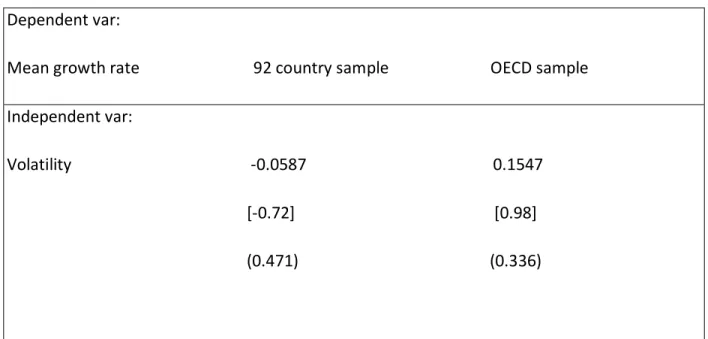
As the results of the regression show on table 1.0, there is a weak negative relationship between volatility and growth. Contrary to the results obtained by Ramey and Ramey (1995), this relationship is statistically highly insignificant as evidenced with a t-statistic of -0.72 and a p-value of 0.47. For the OECD country sample, there is a weak positive relationship which is also statistically insignificant. The t-statistic is 0.98 and the p-value is 0.33. These results though weak in statistical sense still support those obtained by earlier researchers (Ramey and Ramey (1995), AABM(2005)). Henceforth, we examine the relationship between volatility and growth while taking into consideration important specific country characteristics (L-R variables). These variables are the average investment share of GDP, human capital, initial log of GDP per capita, and the average growth rate of the population. As shown in the regression results of table 2.0, including these variables in the model, we realize that in the 92 country sample, all the explanatory factors are insignificant with the sign between volatility and growth reversed also. The only variable that shows a relative strength of significance is the human capital variable with a t-statistic of -1.58. For the OECD sample, we notice that virtually all the variables are statistically insignificant with the exception of human capital which is highly significant with a t-statistic of 2.79. Interesting for this sample, the sign of the relationship stays unchanged as opposed to the 92 country sample. We now introduce the financial development variable in the model as AABM (2005), we realize that all the variables are insignificant in explaining growth in both the 92 country sample and the 24 OECD countries. This shows that financial development is not important in explaining the growth experienced in countries with highly developed financial systems. This result contradicts earlier findings by Ramey and Ramey (1995), and AABM (2005) who have shown that the relationship between growth and volatility is less financial developed economies is negative.
21
Interestingly, we find that the investment variable is not important in explaining growth in both the 92 country sample and the 24 OECD countries. This is also a contradiction to the investment theory.
Table 1.0: For the 92 country sample and the OECD country sample Dependent var:
Mean growth rate 92 country sample OECD sample Independent var:
Volatility -0.0587 0.1547 [-0.72] [0.98] (0.471) (0.336)
Where values in square brackets represent the t-statistics and those in parenthesis represent p-values.
22
Table 2.0: Investigates the volatility-growth relationship while incorporating country specific characteristics for 92 country sample and the OECD sample
Dependent var:
Average growth rate 92 sample OECD sample Independent var: Volatility 0.0175 0.2091 [0.20] [1.40] (0.84) (0.18) Investment 3.261 2.3 [1.61] [1.66] (0.11) (0.12) Initial log gdp 0.717 0.1090 [1.23] [0.16] (0.22) (0.86) Humancapital -0.1392 0.3547 [-1.58] [2.79] (0.12) (0.01) Population growth -29.01 -2.186 [-1.09] [-0.14]
23
Table 3.0: Controlling for the level of financial development of the specific country Dependent var:
Average growth rate 92 sample OECD sample
Independent var: Volatility 0.011 0.2380 [0.10] [1.42] Investment 2.709 2.387 [1.43] [1.60] Initial log gdp -0.133 -0.098 [-0.22] [-0.11] Humancapital -0.144 0.3466 [-1.76] [2.57] Population growth -23.69 -1.703 [-0.96] [-0.10] Financial 1.84 0.518 [1.17] [0.50] Financial*Priv 0.1376 -0.1231 [0.54] [-0.45]
24 7. Concluding Remarks
This rapport has reproduced existing facts also found by other authors. The main lessons we have learned here include the following:
First, for economist to separate real business cycles from economic growth would be a very big error. We find evidence that in fact the there is a relationship between volatility and growth though this relationship is weak in statistical power. Indeed, these two variables are either related in a weak or positive sense depending on specific country characteristics.
Second, we also find as previous researchers that investment is not an important factor in explaining economic growth. It fails in both the 92 country sample and the OECD sample as well. This fact is a complete contradiction to existing investment theory which posits that higher investment leads to higher growth rates and invariably lowers the volatility also.
Third and finally, we conclude that though these results are weak in statistical significance, there are in line with Ramey and Ramey (1995) work which stipulates that volatility is negatively correlated with growth.
25 References
1 Acemoglu D. (2009). Introduction to Economic Growth, Princeton University Press.
2 Aghion P., Angeletos G.M.,Banerjee A. and Manova K. (2005). “Volatility and Growth:
3 Financial Development and the Cyclical Behavior of the Composition of Investment”, Mimeo, Harvard University.
4 Aghion P. and Saint-Paul G. (1998). “Uncovering Some Causal Relationships Between Productivity Growth and the Structure of Economic Fluctuations: A tentative survey”. Labor, 12, 279-303.
5 Ahmet F. (2006). The Effects of Volatility on Growth and Financial Development Through Capital Market Imperfections, MPRA, Working Paper No 5486.
6 Antonio F. (2002). The Effects of Business Cycles on Growth, Central Bank of Chile, Working Paper, No 156.
7 Charles N. and Charles P. (1982). “Trends and Random Walk in Macroeconomic Time Series: Some Evidence and Implications”, Journal of Monetary Economics, 10(2).
8 John L. and Charles P. (1983).”Real Business Cycles” Journal of Political Economy, 91(1).
9 Kydland F. and Edward P. (1982). “Time to build and Aggregate Fluctuations”, Econometrica, 50, 1345-1371.
10 Kory Kroft and Huw Lloyd-Ellis. (2002). “Further Cross-Country Evidence on the Linkage Between Growth, Volatility and Business Cycles, University of California, Berkeley and Queen’s university, Working Paper Series in Economics.26