HAL Id: hal-00781104
https://hal-imt.archives-ouvertes.fr/hal-00781104
Submitted on 25 Jan 2013
HAL is a multi-disciplinary open access
archive for the deposit and dissemination of
sci-entific research documents, whether they are
pub-lished or not. The documents may come from
teaching and research institutions in France or
abroad, or from public or private research centers.
L’archive ouverte pluridisciplinaire HAL, est
destinée au dépôt et à la diffusion de documents
scientifiques de niveau recherche, publiés ou non,
émanant des établissements d’enseignement et de
recherche français ou étrangers, des laboratoires
publics ou privés.
Performance of CSMA in multi-channel wireless
networks
Thomas Bonald, Mathieu Feuillet
To cite this version:
Thomas Bonald, Mathieu Feuillet. Performance of CSMA in multi-channel wireless networks.
Queue-ing Systems, SprQueue-inger Verlag, 2012, 72 (1-2), pp.139-160. �hal-00781104�
arX
iv:
subm
it
/0224029 [c
s.N
I] 2 A
pr 2011
Performance of CSMA in Multi-Channel Wireless Networks
∗
Thomas Bonald
†and Mathieu Feuillet
‡April 2, 2011
Abstract
We analyze the performance of CSMA in multi-channel wireless networks, accounting for the random nature of traffic. Specifically, we assess the ability of CSMA to fully utilize the radio resources and in turn to stabilize the network in a dynamic setting with flow arrivals and departures. We prove that CSMA is optimal in ad-hoc mode but not in infrastructure mode, when all data flows originate from or are destined to some access points, due to the inherent bias of CSMA against downlink traffic. We propose a slight modification of CSMA, that we refer to as flow-aware CSMA, which corrects this bias and makes the algorithm optimal in all cases. The analysis is based on some time-scale separation assumption which is proved valid in the limit of large flow sizes.
Keywords: Wireless network, interference graph, CSMA, flow-level dynamics, time-scale separation, stability.
1
Introduction
The CSMA (Carrier Sense Multiple Access) algorithm is a key component of IEEE 802.11 networks. While it proves successful in sharing a single radio channel between a limited number of stations, its efficiency is questionable in more involved environments with multiple radio channels and a large number of stations having different interference constraints. In this paper, we analyse the ability of CSMA to fully utilize the radio resources in such environments, in both ad-hoc and infrastructure modes, accounting for the random nature of traffic. Specifically, each station attempts to access a randomly chosen radio channel after some random backoff time and transmits a packet over this channel if it is sensed idle. We study the random variations of the number of active wireless links induced by this random access algorithm and the random activity of users. In particular, we analyse the ergodicity of the associated Markov process, which characterizes the ability of CSMA to stabilize the network.
It turns out that, while CSMA is always efficient in ad-hoc mode, in the sense that the network is stable whenever possible, it is generally inefficient in infrastructure mode, when all data flows originate from or are destined to some finite set of access points. This is due to the inherent bias of CSMA against downlink traffic, from the access points to the stations: each access point attempts to access the radio channels with the same rate, independently of the number of active downlink flows at this access point. We prove that a slight modification of CSMA, which consists in running one instance of CSMA per flow at each access point, corrects this bias and makes the algorithm optimal. We refer to this algorithm, introduced in [6], as flow-aware CSMA.
The rest of the paper is organized as follows. We present some related work in the next section. The network model in ad-hoc mode is described in section 3. Sections 4 and 5 are devoted to the packet- and flow-level dynamics, respectively, assuming time-scale separation. The main result
∗A preliminary version of this paper was presented at CISS 2011 [7].
†T. Bonald is with the Department of Computer Science and Networking, Telecom ParisTech, Paris, France.
Email: [email protected]
of the paper, given in Theorem 1, shows in particular the optimality of CSMA in ad-hoc mode. The validity of the time-scale separation assumption is discussed in section 6. The infrastructure mode is considered in section 7, where we prove the suboptimality of standard CSMA and the optimality of flow-aware CSMA. Section 8 concludes the paper.
2
Related work
The present work is related to the problem of optimal scheduling in wireless networks. While a centralized solution is known since the seminal work of Tassiulas and Ephremides, who proved in [24] the optimality of the maximum weight policy, no distributed solution was known until the recent works of Jiang, Ni, Shah and Walrand [11, 12, 20]. These authors considered a simple CSMA algorithm whereby the attempt rate of each station depends either on the number of queued packets or on some local estimates of the arrival rate and the service rate of packets at the station. Similar ideas are used by Ni, Tan and Srikant in [18]. The proof of optimality relies on the fact that these adaptive versions of CSMA achieve the maximum weight scheduling, under some technical assumptions related to the speed of convergence of the algorithm. In practice, the algorithm must indeed be carefully designed so as to enforce the time-scale separation, as shown for instance in the recent paper of Prouti`ere, Yi, Lan and Chiang [19].
All these papers focus on the packet-level dynamics, assuming packets are generated by some fixed number of flows. The flow-level dynamics are ignored, whereas they are known to be critical, see for instance [1, 2, 3, 16] in the context of wireline networks. As in our previous paper [6], we consider both the packet- and flow-level dynamics, under the usual assumption that the former are much faster than the latter. Specifically, we extend the results of [6] to multi-channel networks in both ad-hoc and infrastructure modes and discuss the validity of the time-scale separation assumption.
Surprisingly, little attention has so far been paid to multi-channel networks. A notable ex-ception is the adaptive, multi-channel version of CSMA introduced in [19], which is shown to maximize the network utility when combined with some appropriate virtual queue mechanism. We here prove the optimality of CSMA in the sense of flow-level stability for a very general model where the interference constraints may depend on the considered channel and each transmitter may only use a subset of the channels. Specifically, we show that it is sufficient for each transmitter to probe one of its channels at random, without any further information on the network state.
Another salient feature of this paper is the observation of the key difference between the ad-hoc and infrastructure modes. In the former, the number of transmitters grows with the congestion, which increases the channel attempt rate and in turn stabilizes the network. This is not the case of the latter since the channel access opportunities of each access point must be shared by all downlink flows at this access point. This inherent bias of CSMA against downlink traffic is well known, see e.g. [10, 14], and can be easily corrected by letting the attempt rate of each access point depend on the number of downlink flows, a scheme we refer to as flow-aware CSMA [6]. The algorithm is then optimal.
3
Model
3.1
A multi-channel wireless network
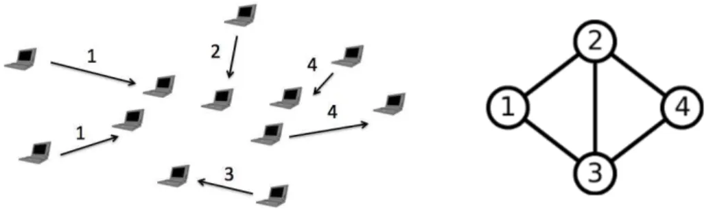
The network consists of a random, dynamic set of wireless links in ad-hoc mode (there is no access point at this stage). These links must share some finite number J of non-interfering radio channels. Each link consists of a transmitter-receiver pair; the transmitter is able to use at most one radio channel at a time. We group links into a finite number of K classes, as illustrated by Figure 1. All links within the same class have the same radio conditions, the same interference constraints and the same CSMA parameters. We denote by xk the number of class-k links and
by x the corresponding vector, which we refer to as the network state. Two links within the same class cannot be simultaneously active on the same channel. An active class-k link on channel j
transmits data at the physical rate ϕk bit/s, independently of j. We say that class k is active on
channel j if there is an active class-k link on channel j.
Figure 1: An ad-hoc wireless network with 4 classes of links and its interference graph. Each channel j is associated with some conflict graph Gj= (Vj, Ej), where Vj ⊂ {1, . . . , K} is
the set of classes that are able to transmit on channel j and Ejis the set of edges, each representing
a conflict. Specifically, two classes k, l ∈ Vj can be simultaneously active on channel j if and only
if they do not conflict with each other, that is if (k, l) $∈ Ej. The J conflict graphs are typically
the same but could differ due to different radio propagation environments on the J channels, or to different transmission capabilities of the K classes.
3.2
Feasible schedules
We refer to a schedule as any vector y ∈ {0, 1}K×J, where y
kj = 1 if class k is active on channel
j. We denote by yk the number of active class-k links:
yk= J
!
j=1
ykj.
The schedule is feasible if for all j = 1, . . . , J, the active classes on channel j belong to Vj and do
not conflict with each other, that is ykjylj= 0 for all (k, l) ∈ Ej. Moreover, we must have:
∀k = 1, . . . , K, yk ≤ xk. (1)
We denote by Y(x) the set of feasible schedules. Note that if xk ≥ J for all k = 1, . . . , K, the
constraint (1) is no longer limiting (since the number of active class-k links is limited by the number of radio channels J) and the set of feasible schedules becomes independent of the network state. We denote by Y the corresponding set, which is the union of Y(x) over all network states x.
3.3
Capacity region
Assume that each feasible schedule y is selected with probability π(y), with "
y∈Yπ(y) = 1. The
mean throughput of class k is then given by: φk= ϕk
!
y∈Y
ykπ(y). (2)
Let φ be the corresponding throughput vector. We refer to the capacity region as the set of vectors φ generated by all probability measures π(y), y ∈ Y. Note that the capacity region depends both on the physical rates and on the interference constraints of all wireless links.
4
Packet-level dynamics
We first analyze the packet-level dynamics induced by CSMA for a static network state x. The flow-level dynamics that make x vary are introduced in section 5.
4.1
Random access
We consider the standard CSMA algorithm where each transmitter waits for a period of random duration referred to as the backoff time before each transmission attempt. At each attempt, the transmitter chooses a radio channel at random and probes it. If the radio channel is sensed idle (in the sense that no conflicting link is active), a packet is transmitted (we neglect tho channel after some random backoff time and transmits a packet over this channel if it is sensed idle. We study the random variations oe collisions); otherwise, the transmitter waits for a new backoff time before the next attempt.
Packets have random sizes of unit mean and are transmitted at the physical rate ϕk on class-k
links; the backoff times of class-k transmitters are random with mean 1/νk , where νk > 0 is the
corresponding attempt rate. We denote by αk= νk/ϕk the ratio of the mean packet transmission
time to the mean backoff time of class-k links. Channel j is chosen with probability βkj, with
"J
j=1βkj = 1 and βkj > 0 if and only if k ∈ Vj, so that all accessible channels are attempted with
positive probability.
4.2
Stationary distribution
Let Y (t) be the schedule selected by the above random access algorithm at time t. We look for the stationary distribution of Y (t), which we denote by π(x, y) to highlight the fact that it depends on the network state x. We have:
Proposition 1. If both the packet sizes and the backoff times have exponential distributions, then Y (t) is a reversible Markov process, with stationary measure:
w(x, y) = # k:xk>0 xk! (xk− yk)! αyk k J # j=1 βykj kj , y ∈ Y(x). (3)
Proof. Let ekj be the unit vector on component k, j on {0, 1}K×J. The Markov process Y (t)
jumps from state y to state y + ekj with rate (xk− yk)νkβkj (since all idle links attempt to access
the channel) and from state y + ekj to state y with rate ϕk (since all class-k links have the same
physical rate ϕk, independently of the used channel), for any state y such that y + ekj ∈ Y(x).
The proof then follows from the local balance equations:
w(x, y)(xk− yk)νkβkj = w(x, y + ekj)ϕk.
! The stationary distribution π(x, y) follows from the normalization of the stationary measure w(x, y) over all y ∈ Y(x). We deduce the mean throughput of class k in state x:
φk(x) = ϕk
!
y∈Y
ykπ(x, y). (4)
It turns out that, by the insensitivity property of the underlying loss network [5], these expressions are in fact valid for any phase-type distributions of packet sizes and backoff times; such distributions are known to form a dense subset within the set of all distributions with real, non-negative support [23], so that the results hold for virtually any distributions of packet sizes and backoff times. We refer the reader to [25] for further details on this insensitivity property.
5
Flow-level dynamics
We now introduce the flow-level dynamics under the assumption of infinitely fast packet-level dynamics; the validity of this time-scale separation assumption is discussed in section 6.
5.1
Traffic characteristics
We assume that flows using class-k links are generated according to a Poisson process of intensity λk. Each such flow has an exponential size with mean σk bits and leaves the network once the
corresponding data transfer is completed. There is a one-to-one correspondence between flows and links so that both terms are used interchangeably in the following. We denote by ρk = λkσk the
traffic intensity of class k (in bit/s) and by ρ the corresponding vector.
Under the time-scale separation assumption, the flow-level dynamics are much slower than the packet-level dynamics so that, at the time scale of a flow, everything happens as if the stationary distribution (3) of the packet-level dynamics were reached instantaneously. In particular, the mean throughput of class k is given by (4) in state x.
5.2
Stability region
Let Xk(t) be the number of class-k flows at time t. The corresponding vector X(t) describes the
evolution of the network state. This is a Markov process with transition rates λk from state x to
state x + ek and φk(x)/σk from state x to state x − ek (provided xk > 0), where ek denotes the
unit vector on component k.
We say that the network is stable if this Markov process is ergodic. Clearly, a necessary condition for stability is that the vector of traffic intensities ρ lies in the capacity region. The following key result of the paper shows that this condition is in fact sufficient, up to the critical case where ρ lies on the boundary of the capacity region. In this sense, CSMA is optimal in the considered ad-hoc mode.
Theorem 1. The network is stable for all vectors of traffic intensities ρ in the interior of the capacity region.
The proof is deferred to the appendix. It is based on the fact that the random access algorithm selects schedules in proportion to their weights (3). For large x, this is equivalent to selecting schedules in proportion to the following uniform weight, which is independent of the channel probing distribution: u(x, y) = # k:xk>0 (xkαk)yk, y ∈ Y(x). (5) Defining: u(x) = max
y∈Y(x)u(x, y),
the following result, also proved in the appendix, shows that those schedules of maximum weight are actually selected with probability close to 1:
Lemma 1. For any ǫ > 0, we have: !
y∈Y(x)
π(x, y) log(u(x, y)) ≥ (1 − ǫ) log(u(x))
for all states x but some finite number.
The result then follows from the stable behavior of maximum weight scheduling, except that the latter is defined over the set of all feasible schedules. Defining the corresponding weight by:
v(x) = max
y∈Y u(x, y),
the following result, proved in the appendix, shows that it is essentially the same as u(x): Lemma 2. We have:
sup
x∈X
v(x) u(x) < ∞.
6
Time-scale separation
Theorem 1 is based on the time-scale separation assumption: in the packet-level model of section 4, packets “see” a fixed number of flows, while in the flow-level model of section 5, flows “see” the equilibrium state of packet-level dynamics. In this section, we remove this assumption. Specif-ically, we prove that when the size of the flows grows, the model without time-scale separation converges to the model with time-scale separation, which indeed suggests that CSMA is optimal for sufficiently large flow sizes. We actually conjecture that CSMA is optimal for any flow size, which we prove at the end of the section for a specific class of networks.
6.1
Scaling
As in section 5, class−k flows are assumed to arrive according to a Poisson process of intensity λk. The number of packets per class-k flow has a geometric distribution with mean N σk, where
N is some positive integer, we refer to as the scaling parameter. In particular, each class-k flow terminates with probability 1/(σkN ) after each packet transmission. Packets are assumed to have
an exponential size with mean 1/N bits, so as to keep the class-k mean flow size constant and equal to σk bits. In particular, the corresponding traffic intensity ρk= λkσk is independent of N .
The random access algorithm is that described in section 4.1. The only difference is that the attempt rates must be scaled so as to keep the ratio of mean packet transmission time to mean backoff time constant. Thus each class-k link now attempts to access the channels at rate N νk.
6.2
Asymptotic time-scale separation
The state of the network is now described by the couple (XN(t), YN(t)), where XN(t) gives the
number of flows of each class at time t and YN(t) the schedule that is selected at time t. This
is a Markov process with transition rates λk from state (x, y) to state (x + ek, y) (class-k flow
arrival), N (xk− yk)νkβkj from state (x, y) to state (x, y + ekj) (access to channel j by a class-k
flow), N ykjϕk(1 − 1/(σkN )) from state (x, y) to state (x, y − ekj) (packet transmission of a class-k
flow over channel j, without flow completion), ykjϕk/σk from state (x, y) to state (x − ek, y − ekj)
(packet transmission of a class-k flow over channel j, with flow completion).
When N grows, the packet-level dynamics, represented by YN(t), are accelerated with respect
to the flow-level dynamics, represented by XN(t). The following result, proved in the appendix,
shows that there is indeed time-scale separation between the packet level and the flow level in the limit. We assume that XN(0) = X(0) for all N ≥ 1.
Theorem 2. When N → ∞, the stochastic process XN(t) converges in distribution to the Markov
process X(t), which describes the network state under the time-scale separation assumption.
6.3
Stability of some class of networks
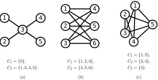
Theorems 1 and 2 suggest that CSMA is optimal for sufficiently large flow sizes. We conjecture that CSMA is actually optimal for any flow size, in the sense that the Markov process (XN(t), YN(t))
is ergodic for any scaling parameter N ≥ 1 provided the vector of traffic intensities ρ lies in the interior of the capacity region. To support this conjecture, consider the following class of networks. We assume that all links have access to the J channels. The interference graph is the same on all channels and given by some L-partite graph, i.e. there exists a partition {C1, . . . , CL}
of {1, . . . , K} such that two classes in Cl do not interfere with each other but a class in Cl does
interfere with all classes in {1, . . . , K} \ Cl. Examples of L-partite graphs are given in figure 2.
The following result, proved in the appendix, shows that CSMA is optimal independently of the scaling parameter N :
Proposition 2. Any network with a L-partite interference graph is stable for all vectors of traffic intensities ρ in the interior of the capacity region.
C1= {3}, C2= {1, 2, 4, 5}. (a) C1= {1, 2, 3}, C2= {4, 5, 6}. (b) C1= {1, 2}, C2= {3, 4}, C3= {5}. (c) Figure 2: Examples of 2-partite (a)-(b) and 3-partite (c) graphs.
7
Infrastructure-based networks
We have so far considered a network in ad-hoc mode, without infrastructure. We now consider N access points to which users must connect. In particular, each class now corresponds either to uplink traffic (from the users to an access point) or to downlink traffic (from an access point to the users). We study the flow-level dynamics of CSMA under the time-scale separation assumption. Specifically, we prove the suboptimality of standard CSMA in this context and introduce a slight modification of CSMA, we refer to as flow-aware CSMA, which makes the algorithm optimal.
7.1
Uplink vs. downlink
For all i = 1, . . . , N , we denote by Uiand Di the sets of uplink and downlink classes, respectively,
associated with access point i. In the example of figure 3, for instance, there are N = 2 access points and K = 6 classes, with U1 = {2}, D1 = {1, 3}, U2 = {5} and D2 = {4, 6}. An access
point cannot transmit and receive on the same channel. In particular, those classes sharing the same access point, either in uplink or downlink, conflict with each other. Formally, for all access points i = 1, . . . , N and all classes k, l ∈ Ui∪ Di, we have (k, l) ∈ Ej for each channel j such that
k, l ∈ Vj. We assume that an access point cannot transmit data on more than one channel at a
time but is able to receive data on the J channels simultaneously.
Figure 3: A network of 2 access points with 6 classes of links and its interference graph. The feasible schedules are those defined in section 3.2, with the additional constraint that each access point cannot transmit data on more than one channel at a time, that is:
∀i = 1, . . . , N, !
k∈Di
We denote by Y(x) the set of feasible schedules and by Y the union of Y(x) over all network states x. The corresponding capacity region is defined in section 3.3.
7.2
Standard CSMA
We first consider the standard CSMA algorithm: each transmitter waits for a period of random duration before attempting transmission on some randomly chosen channel. The key difference with the ad-hoc wireless network considered so far is that each access point runs a single instance of the CSMA algorithm for all its downlink traffic. In particular, for each access point i, the attempt rates νk are the same for all classes k ∈ Di. At each attempt, the access point i selects a
class-k flow with some probability proportional to xk and probes channel j with probability βkj.
If the probed channel is sensed idle, a packet of this flow is transmitted.
It is worth noting that the attempt rate of each access point is independent of its congestion level, in terms of the number of ongoing downlink flows at this access point. This breaks the natural stabilizing effect of CSMA we have proven in Theorem 1 in the context of ad-hoc networks, where those classes with a higher number of flows get preferential access to the radio channels. In the following, we illustrate the suboptimality of standard CSMA on two examples with downlink traffic only. Note that, in the presence of uplink traffic only, the model is in fact equivalent to the ad-hoc network considered so far.
For this purpose, we give the distribution of feasible schedules achieved by the algorithm under the time-scale separation assumption. Denoting by Y (t) the schedule at time t, we have the analogue of Proposition 1:
Proposition 3. If both the packet sizes and the backoff times have exponential distributions, then Y (t) is a reversible Markov process, with stationary measure:
w(x, y) = N # i=1 # k∈Ui:xk>0 xk! (xk− yk)! αyk k J # j=1 βykj kj × $ ! k∈Di xk % ! # k∈Di:xk>0 αyk k xk! J # j=1 βykj kj , y ∈ Y(x). (7)
Proof. As for Proposition 1, the proof follows from the local balance equations. For all i, . . . , N , we have: ∀k ∈ Ui, w(x, y)(xk− yk)νkβkj = w(x, y + ekj)ϕk, and ∀k ∈ Di, w(x, y) xk " k∈Dixk νkβkj= w(x, y + ekj)ϕk. !
The stationary distribution of the schedules π(x, y) follows from normalization. Again, it is insensitive to the packet size and backoff time distributions beyond the means. The throughput of class k is given by (4).
Example 1 The most simple example showing the suboptimality of CSMA is shown in Figure 4. It consists of N = 3 access points, a single class per access point and a single channel. Taking unit physical rates, the optimal stability region is ρ1+ ρ2< 1 and ρ2+ ρ3< 1 where 1 and 3 are
the edge classes and 2 is the center class. We have proven in [6] that the actual stability region is strictly smaller, even in the limiting case of infinite attempt rates.
Figure 4: Network of 3 access points with a single downlink class per access point and its inter-ference graph.
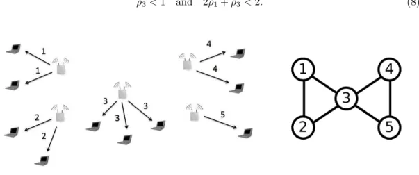
Example 2 Consider the multi-channel network of Figure 5 with N = 5 access points, a single class per access point and J = 2 channels, further referred to as the bow tie network. The conflict graph is the same for both channels. We refer to class 3 as the center class and to the other classes as the edge classes. We assume that the mean packet sizes and the mean backoff times are the same for all classes, so that αk = α for all k = 1, . . . , 5, for some α > 0. We also assume that
all classes except class 3 have the same traffic intensities. The optimal stability condition is then given by:
ρ3< 1 and 2ρ1+ ρ3< 2. (8)
Figure 5: Network of 5 access points with a single downlink class per access point and its inter-ference graph.
We consider the limiting case where α → ∞ and we assume that the two channels are chosen uniformly at random. We then deduce from (3)-(4) the following throughput vector:
φ(x) = (1, 1, 0, 1, 1) if x1, x2, x4, x5> 0, *3 4, 3 4, 1 2, 1, 0 + if x1, x2, x3, x4> 0, x5= 0, *2 3, 2 3, 2 3, 0, 0 + if x1, x2, x3> 0, x4= x5= 0, (0, 1, 1, 1, 0) if x2, x3, x4> 0, x1= x5= 0, (1, 1, 0, 0, 0) if x1, x2> 0, x3= x4= x5= 0, (1, 0, 0, 0, 0) if x1> 0, x2= 0, x3= x4= x5= 0. (9)
The other cases follow by symmetry. The center class is in conflict with all other classes for accessing the channels and is either not served when the 4 other classes are active or served at a low rate when 3 other classes are active. This also results in a suboptimal stability region: Proposition 4. The bow tie network is unstable whenever:
ρ3> 1 3ρ 4 1− 2 3ρ 3 1− 2 3ρ 2 1+ 1. (10)
This proposition is proven in the appendix. In the homogeneous case ρ1 = ρ3 for instance,
Proposition 4 implies that the network is unstable whenever ρ1> 0.63. In view of (8), the optimal
stability condition is ρ1 < 2/3, which shows that the standard CSMA algorithm is not optimal.
This suboptimality is illustrated by Fig. 6, the actual stability condition being obtained by the simulation of the underlying Markov process. In the homogeneous case for instance, the loss of efficiency is around 15%. 0 0.2 0.4 0.6 0.8 1 0 0.2 0.4 0.6 0.8 1 C e n te r lin k lo a d
Edge link load Optimal stability region
Actual stability region
Figure 6: Stability region of the bow-tie network with two channels under standard CSMA.
7.3
Flow-aware CSMA
The flow-aware CSMA algorithm consists for each access point to run one standard CSMA algo-rithm per flow. This compensates for the inherent bias of standard CSMA against downlink flows and stabilizes the network whenever possible. Indeed, the stationary measure of the schedules is now given by (3). The only difference with the ad-hoc wireless network considered in section 5 is the additional constraint (6) on the set of feasible schedules. This does not change the proof of Theorem 1, showing the optimality of flow-aware CSMA.
8
Conclusion
We have proved that, under the time-scale separation assumption, the distributed scheduling achieved by standard CSMA exploits the radio resources in an optimal way in ad-hoc wireless networks. This is not the case in the presence of access points, due to the inherent bias of CSMA against downlink traffic. A slight modification of CSMA we refer to as flow-aware CSMA is then sufficient to correct this bias and to make the algorithm optimal.
The analysis relies on a number of simplifying assumptions that we plan to relax in future work. First, we have neglected the impact of packet collisions; these could be included in the model, as done in [13] for rate-based adaptive CSMA for instance. One may then account for the adaptive backoff of the IEEE 802.11 protocol, which is key in practice to limit the number of collisions. Other issues that may be worth addressing concern the traffic model. We have neglected the impact of acknowledgements, which are known to be critical in IEEE 802.11 networks. The impact of real-time traffic should also be considered. Finally, one may think of multi-hop networks where the flows of some source-destination pairs must go through one or several relay nodes. Although we believe that flow-aware CSMA is still optimal in this more general settings, we have not yet been able to prove this result.
From a more theoretical perspective, one may relax the assumption of Poisson flow arrivals and exponential flow sizes in the stability analysis. One may for instance consider user sessions that consist of an alterning series of file transfers and idle periods. We would also like to extend Proposition 2 to any interference graph, which would prove the validity of Theorem 1 in the absence of the time-scale separation assumption.
Appendix
Proof of Lemma 1 For any class k, let:
βk= min
j:k∈Vj
βkj.
Note that βk> 0. We have for all y ∈ Y(x):
w(x, y) ≥ # k:xk>0 xk(xk− 1) . . . (xk− yk+ 1) xyk k βJ ku(x, y). If xk ≤ 2J, we have: xk(xk− 1) . . . (xk− yk+ 1) xyk k ≥ 1 xyk k ≥ 1 (2J)J.
Otherwise, we have using the fact that yk ≤ J for all k = 1, . . . , K:
xk(xk− 1) . . . (xk− yk+ 1) xyk k ≥, xk− yk+ 1 xk -yk ≥ 1 2J.
Combining these results, we obtain the existence of some constant m > 0 such that: ∀y ∈ Y(x), w(x, y) ≥ mu(x, y).
Now let:
Z(x) =.y ∈ Y(x) : log(u(x, y)) ≥ (1 − ǫ
2) log(u(x)) / . We have: ! y∈Z(x) π(x, y) log(u(x, y)) ≥ (1 − ǫ 2) log(u(x)) ! y∈Z(x) π(x, y).
Using the fact that w(x, y) ≤ u(x, y) for all y ∈ Y(x), we get:
! y∈Y(x)\Z(x) π(x, y) = " y∈Y(x)\Z(x)w(x, y) " y∈Y(x)w(x, y) , ≤ 1 m " y∈Y(x)\Z(x)u(x, y) " y∈Y(x)u(x, y) , ≤ 1 m M u(x)1−! 2
maxy∈Y(x)u(x, y)
,
= 1 m
M u(x)!2,
where M denotes the total number of schedules (that is, the cardinal of Y). Since u(x) tends to +∞ when |x| ≡"
kxk tends to +∞, this quantity is less than ǫ/2 for all states x but some finite
number. In those states, we have:
!
y∈Z(x)
π(x, y) ≥ 1 − ǫ 2.
We deduce that in all states x but some finite number: ! y∈Y(x) π(x, y) log(u(x, y)) ≥ (1 − ǫ 2) 2log(u(x)), ≥ (1 − ǫ) log(u(x)). ! Proof of Lemma 2 Let:
v(x, y) = #
k:xk≥J
(xkαk)yk.
There are some positive constants m, M such that:
∀x ∈ NK, ∀y ∈ Y, m ≤ u(x, y) v(x, y) ≤ M. The proof then follows from the fact that:
v(x) = max
y∈Y u(x, y) ≤ M maxy∈Y v(x, y) = M maxy∈Y(x)v(x, y) ≤
M
m y∈Y(x)max u(x, y) =
M mu(x).
! Proof of Theorem 1 If the vector of traffic intensities lies in the interior of the capacity region, there exist some ǫ > 0 and some probability measure π on Y such that:
∀k = 1, . . . , K, ρk = ϕk(1 − 2ǫ)
!
y∈Y
π(y)yk. (11)
Note that we can choose π(y) > 0 for all y ∈ Y. Define the Lyapunov function:
F (x) = !
k:xk>0
xkσk
ϕk
log(xkαk).
The corresponding drift is given by:
∆F (x) =! k λk(F (x + ek) − F (x)) + ! k:xk>0 φk(x) σk (F (x − ek) − F (x)), = ! k:xk=0 ρk ϕk log(αk) + ! k:xk>0 ρk ϕk ((xk+ 1) log((xk+ 1)αk) − xklog(xkαk)) + ! k:xk>0 φk(x) ϕk ((xk− 1) log((xk− 1)αk) − xklog(xkαk)) .
In particular, we have ∆F (x) = G(x) + H(x) with:
G(x) = ! k:xk>0 ρk− φk(x) ϕk log(xkαk), H(x) = ! k:xk>0 ρk ϕk (xk+ 1) log(1 + 1 xk ) + ! k:xk>0 φk(x) ϕk (xk− 1) log(1 − 1 xk ) + ! k:xk=0 ρk ϕk log(αk),
where we use the convention 0 log(0) ≡ 0. Since φk(x) ≤ Jϕk, the function H(x) is bounded.
Regarding G(x), it follows from (5) and (11) that: G(x) =! y∈Y ((1 − 2ε)π(y) − π(x, y)) ! k:xk>0 yklog(xkαk), =! y∈Y
((1 − 2ε)π(y) − π(x, y)) log(u(x, y)).
By Lemma 1, we have for all states x but some finite number:
G(x) ≤ −ǫ!
y∈Y
π(y) log(u(x, y)) + (1 − ǫ)
!
y∈Y
π(y) log(u(x, y)) − log(u(x)) ,
≤ −ǫ!
y∈Y
π(y) log(u(x, y)) + (1 − ǫ) log, v(x) u(x)
-.
Since π(y) > 0 for all y ∈ Y, the first term tends to −∞ when |x| ≡ "
kxk tends to +∞.
By Lemma 2, the second term is bounded. We deduce the existence of some δ > 0 such that ∆F (x) ≤ −δ for all states x but some finite number. The proof then follows from Foster’s
criterion. !
Proof of Theorem 2 In the following, we consider (XN(t))
N≥1 as a sequence of stochastic
processes in the space DNK([0, ∞[) of c`ad-l`ag functions with values in NK with the Skorohod
topology.
First, we have to prove the tightness of the sequence (XN(t)). It is enough to remark that, for
all N ≥ 1, XN
k (t) is stochastically dominated by a Poisson process of intensity λkand stochastically
dominates an M/M/1 queue with arrival rate λk and service rate ϕk/σk. Thus, the conditions of
the Arzel`a-Ascoli theorem are fulfilled and the sequence (XN(t)) is tight (see [4, Th 12.3]).
We now consider a bounded function f on NK. Denote by ΩN the infinitesimal generator of
the Markov process (XN(t), YN(t)). For x ∈ NK and y ∈ Y, we have
ΩN(f )(x, y) = K ! k=1 λk(f (x + ek) − f (x)) − K ! k=1 ϕk/σk J ! j=1 ykj(f (x − ek) − f (x)).
According to the Martingale characterization of Markov jump processes (see [22]), the process:
MN f (t) = f (X N(t)) − f (XN(0)) −4 t 0 ΩN(f )(XN(s), YN(s)) ds
is a locale martingale and, since the process XN(t) is not exploding on [0, t] (it is stochastically
dominated by a Poisson process), it is a martingale. For each N ≥ 1, define the random measure:
ΓN([0, t] × B) =4 t
0 {Y (s)∈B}
ds, for B ⊂ Y
ΓN is a random variable with value in the set L(Y) of the random measures on [0, ∞[×Y such
that if µ ∈ L(Y) then µ([0, t] × Y) = t for all t ≥ 0. Since Y is finite, the set L(Y) is compact and then the sequence (ΓN)
N≥1 is relatively compact.
Assume that the sequence (XN(t), ΓN)
N≥1 tends to some limit (X(t), Γ). Since:
4 t 0 ΩN(f )(XN(s), YN(s)) ds = 4 t 0 ! y∈Y ΩN(f )(XN(s), y)ΓN(ds × dy)
and f is bounded, this random variable tends in distribution to: 4 t 0 ! y∈Y Ω(f )(X(s), y)Γ(ds × dy).
It remains to characterize Γ. According to Lemma 1.3 of [15], there exists a set of random probability measures ϑ(t, .) on Y such that:
Γ([0, t] × B) = 4 t
0
ϑ(s, B) ds, for B ⊂ Y. For any function g on Y, we define the martingale:
¯ MN g (t) = 1 N , g(YN(t)) − g(YN(0)) − 4 t 0 ΩN(g)(XN(s), YN(s)) ds -.
For x ∈ NK and y ∈ Y, we have:
ΩN(g)(x, y) = K ! k=1 J ! j=1 N (xk− yk)νkβkj(g(y + ekj) − g(y)) + , N ykjϕk , 1 − 1 σkN -+ϕk σk -(g(y − ekj) − g(y)).
The increasing process of this martingale is: 5 ¯ MgN(t)6 = 1 N2 4 t 0 ΩN(g)(XN(s), YN(s)) ds, ≤ 2t
Nmaxy∈Y |g(y)|
, max
k ϕk+ maxk νkmaxk,j βkj
-.
It tends to 0 on all compact sets so that the martingale tends in distribution to 0. Since Y is finite, g is bounded and (g(YN(t)) − g(YN(0)))/N also tends to 0. Finally, we get that:
1 N
4 t
0
ΩN(g)(XN(s), YN(s)) ds
converges in distribution to 0. This implies: 4 t 0 ! y∈Y $K ! k=1 J ! j=1 (Xk(s) − yk)νkβkj(g(y + ekj) − g(y)) + ykjϕk(g(y − ekj) − g(y)) % ϑ(s, y) ds = 0
and for almost every s in [0, t], we have:
! y∈Y $ K ! k=1 J ! j=1 (Xk(s) − yk)νkβkj(g(y + ekj) − g(y)) + ykjϕk(g(y − ekj) − g(y)) % ϑ(s, y) = 0
The probability distribution ϑ(s, .) is then the stationary distribution given by (3). It follows that:
4 t
converges in distribution to:
4 t
0
Ω(f )(X(s)) ds
where Ω is the infinitesimal generator of the Markov process described in section 5. For x ∈ NK,
we have Ω(f )(x) = K ! k=1 λk(f (x + ek) − f (x)) + φk(x)/σk(f (x − ek) − f (x)) ,
where φk(x) is the mean throughput of class k in state x, given by (4).
By dominate convergence, MN
f (t) tends in distribution to:
Mf(t) = f (X(t)) − f (X(0)) −
4 t
0
Ω(f )(X(s)) ds,
and Mf(t) is a martingale. Using the characterization of the Markov jump processes, we get that
the process X(t) is a Markov process with infinitesimal generator Ω.
This concludes the proof. !
Proof of Proposition 2 For this proof, we will need the notion of fluid limits. A fluid limit is a limiting point ¯XN(t) of the laws of the processes {XN(nt)/n, n ≥ 1} in the set of probability
measures on the space DRK
+([0, ∞)) of cad-lag functions with value in R
K
+ with Skorohod topology
(see [4]). It is not difficult to show that the set of processes {XN(nt)/n, n ≥ 1} is tight in the set
of probability distributions on the space DRK
+([0, ∞)) endowed with the metric associated to the
uniform norm on compact sets. Therefore, there exists at least one fluid limit and any fluid limit is continuous. Since the process YN(nt) has its values in a finite space for all n ≥ 1, it can be
proved as in [8, 21] that, if there exists a deterministic time T > 0 such that ¯XN(t) = 0 for all
t ≥ T , then the Markov process (XN(t), YN(t)) is ergodic.
The proof is then very similar to that given in [9] for random capture algorithms. We consider a fluid limit ¯XN(t) and define:
WN(t) = L ! i=1 max k∈Cl , ¯ XN k (t) σk ϕk -.
When some class in Cltakes channel j, all other classes in Clcan take this channel while all classes
in {1, . . . , K} \ Clcannot. This implies:
WN(t) ≤ max $ 0, 1 + $ L ! l=1 max k∈Cl ρk ϕk − J % t % .
In the case of L-partite networks, the capacity region is given by the set of vectors φ such that:
L ! l=1 max k∈Cl φk ϕk ≤ J.
Since ρ lies inside the capacity region, we have WN(t) = 0 for all t ≥ T , with
T = 1 J −"L
i=1maxk∈Clρk
,
which implies the ergodicity of the Markov process (XN(t), YN(t)).
Proof of Proposition 4 Define the throughput vector ˜φ such that ˜φ3(x) = φ3(x) and ˜φk(x) =
{xk>0} for all k $= 3. It can be easily verified that ˜φk(x) ≥ ˜φk(y) for all states x, y such that
x ≤ y and all k such that xk > 0. Now consider the coupling of the stochastic processes X(t) and
˜
X(t) describing the evolution of the queues for the throughputs φ and ˜φ, respectively, starting from the same initial state X(0) = ˜X(0). It follows from the above monotonicity property that
˜
X(t) ≤ X(t) a.s. at any time t ≥ 0. In particular, the transience or the null recurrence of ˜X(t) implies that of X(t).
For the throughput vector ˜φ(t), queues 1,2,4,5 are independent M/M/1 queues with load ρ1.
If ρ1≥ 1, the Markov process ˜X(t) is null recurrent or transient. Note that (10) then reduces to
ρ3≥ 0.
Assume now that ρ1< 1. To prove the transience of ˜X(t), we use fluid limits. Since ρ1< 1 and
for ˜φ(t), queues 1,2,4,5 are independent M/M/1 queues with load ρ1, there exists some finite time
after which, for any initial conditions, the corresponding components of the fluid limit are null. We then just have to consider the fluid limits with the initial condition ¯X3(0) = 1 and ¯Xk(0) = 0
for all k $= 3. In this case, Proposition 9.14 of [21, p.241] applies and the fluid limit satisfies: ¯ X3(t) = 1 + , λ3− ¯ φ3 σ3 -t,
as long as this function is positive, where ¯φ3 is the throughput of link 3 averaged over the states
of other links. Since each other link is active with probability ρ1, it follows from (9) that:
¯ φ3= 1 3ρ 4 1− 2 3ρ 3 1− 2 3ρ 2 1+ 1.
In particular, ¯X3(t) increases linearly to infinity whenever inequality (10) is satisfied and, according
to [17], the Markov process ˜X(t) is transient. !
References
[1] C. Barakat, P. Thiran, G. Iannaccone, C. Diot, and P. Owezarski. Modeling internet backbone traffic at the flow level. IEEE Transactions on Signal processing, 51:2003, 2003.
[2] S. Ben Fredj, T. Bonald, A. Prouti`ere, G. R´egni´e, and J. W. Roberts. Statistical bandwidth sharing: a study of congestion at flow level. In Proceedings of ACM SIGCOMM, pages 111– 122, 2001.
[3] A. W. Berger and Y. Kogan. Dimensioning bandwidth for elastic traffic in high-speed data networks. IEEE/ACM Trans. Netw., 8(5):643–654, 2000.
[4] P. Billingsley. Convergence of Probability Measures (second edition). Wiley Series in Proba-bility and Statistics. Wiley-Interscience, 1999.
[5] T. Bonald. Insensitive traffic models for communication networks. Discrete Event Dynamic Systems, 17(3):405–421, 2007.
[6] T. Bonald and M. Feuillet. On the stability of flow-aware CSMA. Perform. Eval., 67:1219– 1229, November 2010.
[7] T. Bonald and M. Feuillet. On flow-aware CSMA in multi-channel wireless networks. In CISS, 2011.
[8] J. G. Dai. On positive Harris recurrence of multiclass queueing networks: a unified approach via fluid limit models. Annals of Applied Probabilities, 5:49–77, 1995.
[10] M. Heusse, F. Rousseau, G. Berger-Sabbatel, and A. Duda. Performance anomaly of 802.11b. In INFOCOM, volume 2, pages 836–843, 2003.
[11] L. Jiang, D. Shah, J. Shin, and J. Walrand. Distributed random access algorithm: Scheduling and congestion control. IEEE Transactions on Information Theory, 56(12):6182 – 6207, 2011. [12] L. Jiang and J. Walrand. A distributed CSMA algorithm for throughput and utility maxi-mization in wireless networks. In the 46th Annual Allerton Conference on Communication, Control, and Computing, 2008.
[13] Libin Jiang and Jean Walrand. Approaching throughput-optimality in a distributed CSMA algorithm: collisions and stability. In MobiHoc S3’09, pages 5–8. ACM, 2009.
[14] S. W. Kim, B.-S. Kim, , and Y. Fang. Downlink and uplink resource allocation in IEEE 802.11 wireless LANs. IEEE Trans. Veh. Technol., 54:320327, Jan. 2005.
[15] T.G. Kurtz. Averaging for martingale problems and stochastic approximation. In Applied Stochastic Analysis, US-French Workshop, volume 177 of Lecture notes in Control and Infor-mation sciences, pages 186–209. Springer Verlag, 1992.
[16] L. Massouli´e and J. W. Roberts. Bandwidth sharing and admission control for elastic traffic. Telecommunication Systems, 15:185–201, 2000.
[17] S. Meyn. Transience of multiclass queueing networks via fluid limit models. Annals of Applied Probability, 5:946–957, 1995.
[18] J. Ni, B. Tan, and R. Srikant. Q-CSMA: Queue-length based CSMA/CA algorithms for achieving maximum throughput and low delay in wireless networks. In IEEE INFOCOM, 2010.
[19] A. Prouti`ere, Y. Yi, T. Lan, and M. Chiang. Resource allocation over network dynamics without timescale separation. In IEEE INFOCOM, 2010.
[20] S. Rajagopalan, D. Shah, and J. Shin. Network adiabatic theorem: an efficient randomized protocol for contention resolution. In SIGMETRICS’09, pages 133–144. ACM, 2009. [21] P. Robert. Stochastic Networks and Queues. Stochastic Modeling and Applied Probability
Series. Springer-Verlag, New York, 2003.
[22] L. C. G. Rogers and D. Williams. Diffusions, Markov processes & martingales vol. 2: Itˆo Calculus. Cambridge University Press, 2000 (1987).
[23] R. Serfozo. Introduction to Stochastic Networks. Springer-Verlag New York, 1999.
[24] L. Tassiulas and A. Ephremides. Stability properties of constrained queueing systems and scheduling policies for maximum throughput in multihop radio networks. IEEE Transactions on Automatic Control, 37:1936–1948, 1992.
[25] P. M. van de Ven, S. C. Borst, J. S. H. van Leeuwaarden, and A. Prouti`ere. Insensitivity and stability of random-access networks. Perform. Eval., 67:1230–1242, November 2010.