Elections and Economic Policy in Developing Countries

DIAL • 4, rue d’Enghien • 75010 Paris • Téléphone (33) 01 53 24 14 50 • Fax (33) 01 53 24 14 51 E-mail : dial@dial.prd.fr • Site : www.dial.prd.fr

DOCUMENT DE TRAVAIL DT/2008-11

Elections and Economic Policy in

Developing Countries

Lisa CHAUVET

Paul COLLIER

ELECTIONS AND ECONOMIC POLICY IN DEVELOPING COUNTRIES1 Lisa Chauvet

IRD-DIAL, Paris

chauvet@dial.prd.fr

Paul Collier

CSAE, Department of Economics, University of Oxford

paul.collier@economics.ox.ac.uk

Document de travail DIAL Décembre 2008 ABSTRACT

This paper explores the impact of elections on economic policies and governance in developing countries. We distinguish between a structural effect, which increases accountability, and a cyclical effect which may be disruptive. Since the effects are offsetting, neither can be analyzed in isolation. We implement an econometric analysis on more than 80 developing countries using positive changes in the Country Policy and Institutional Assessment of the World Bank and the International Country Risk Guide as signaling improvements in economic policy and governance. We find that both structural and cyclical effects matter. The cyclical effect suggests that mid-term is the best moment for policy change. We investigate the structural effect by comparing different frequencies of elections. Except at the extremes, a higher frequency of elections improves both policy and governance net of any cyclical effect. The important exception to this benign net effect is if the electoral process is badly conducted. Badly conducted elections have no structural efficacy for policy improvement. A reasonable interpretation of our results is that honest elections increase accountability and thereby discipline governments to improve economic policy and governance, but that if candidates can win by fraud this chain is broken.

Keywords: Elections, economic policy, developing countries

RESUME

Cet article analyse l’influence des élections sur les politiques économiques et la gouvernance dans les pays en développement. Nous distinguons un effet structurel des élections – via la responsabilité politique – d’un effet cyclique potentiellement perturbateur. Puisque ces deux effets se compensent, ils ne peuvent être considérés séparément. Nous menons une analyse économétrique sur un échantillon de 80 pays en développement pour identifier l’impact des élections sur l’amélioration des politiques économiques. Nous utilisons les changements positifs du Country Policy and Institutional Assessment de la Banque mondiale et de l’International Country Risk Guide pour saisir les améliorations des politiques économiques et de la gouvernance. Nous trouvons que l’effet structurel et l’effet cyclique des élections sont tous deux importants. L’effet cyclique des élections suggère que les améliorations de politiques économiques sont plus probables à mi-mandat. Nous utilisons la fréquence des élections pour saisir leur effet structurel. Il semble que des élections fréquentes améliorent la qualité des politiques économiques et de la gouvernance, une fois pris en compte leur effet cyclique. Une exception importante à cet effet structurel positif concerne les élections dont le processus est mal mené : elles n’ont dans ce cas pas d’effet structurel positif. Il semble donc que des élections honnêtes augmentent la responsabilité politique des gouvernements et les incitent ainsi à améliorer les politiques économiques et la gouvernance ; mais si le candidat peut gagner par fraude, cette chaine est rompue.

Mots clés : Elections, politique économique, pays en développement

1. INTRODUCTION

This paper investigates whether elections in developing countries have improved economic policies and economic governance. Both casual empiricism and casual theorizing suggest that they have done so. As contested elections have become more common since the 1990s, the policy ratings from the World Bank and the International Country Risk Guide have both improved markedly. These improvements accord with the fundamental notion that elections discipline governments into good performance.

Yet this view from on high often collides with the actual experience of individual elections. The Kenyan election of December 2007 triggered a catastrophic implosion of the society, polarizing it on ethnic lines. To date, the legacy of that election is a policy paralysis: for example, the number of government ministers has been doubled with a resulting loss of policy coherence. In Zimbabwe the prospect of contested elections in 2002 and 2008 clearly failed to discipline President Mugabe into adopting good economic policies: he chose hyperinflation, using the revenues to finance patronage. The most celebrated economic reform episode in Africa is Nigeria 2003-6, when a group of technocrats led by Ngozi Nkonjo-Iweala as Minister of Finance turned the economy around. This episode was ushered in by the replacement of a military dictator, General Abacha, with an elected president, Obasanjo, suggesting that elections indeed improved government performance. However, reform only began in Obasanjo’s second and final term, when he no longer faced the discipline of an election. He told Nkonjo-Iweala that the window for reform was only three years, not the full four years of his term: as he said, ‘the last year will be politics’2_{. Indeed,} that Nigeria failed to harness the first oil boom was primarily the responsibility of a democratic government, elected in 1978. That government adopted very poor economic policies, including borrowing heavily in order to finance public consumption; it was also famously corrupt. Despite its disastrous performance it was re-elected in 1983. As these examples suggest, in the conditions typical of many developing countries, elections may be two-edged swords.

The effect of elections on policy in low-income countries is of considerable importance. Since aid was first used conditionally to promote ‘Structural Adjustment’ in the 1980s the international community has recognized that policy improvement is fundamental to development. During the 1990s the approach to

how good policies should be promoted shifted from conditionality, which was increasingly seen as both

ineffective and unacceptable, to the promotion of democracy. Electorates rather than donors would coerce governments into good performance. At the core of the promotion of democracy was the promotion of elections: for example, in 2006 donors provided $500m to finance elections in the Democratic Republic of the Congo. Yet the premise that elections are effective in such conditions has yet to be evaluated. At a more pragmatic level, since elections periodize political decision taking, they might also periodize policy reform: some times might be ripe for good policy. For example, it would be useful both to political leaders and to donors to know whether the year just prior to an election is indeed unsuited to policy reform as President Obasanjo evidently thought.

There is a large general literature on the relationship between democracy and economic performance but it does not provide much guidance as to these questions. The conclusion from the literature is that any such relationship is weak (Drazen, 2000; Feng, 2003; Przeworski et al., 2000). However, these studies do not focus specifically on the characteristics prevalent in developing countries many of which democratized during the 1990s. Several recent studies find that democracy has distinctive effects in the context of such characteristics. Alesina and La Ferrara (2005) and Collier (2001) focus on the consequences of ethnic diversity for growth. They find that diverse societies benefit significantly more from democracy than homogenous societies. Collier and Rohner (2008) focus on the relationship between democracy and the risk of large-scale political violence. They find that whereas in developed economies democracy increases security, below an income threshold of around $2,700 per capita it significantly increases the risk of political violence. Finally, Collier and Hoeffler (2008) focus on the relationship between democracy and

the economic performance of resource-rich countries. They find that whereas below a threshold of resource wealth democracy is significantly beneficial, above the threshold it significantly worsens performance. These results suggest that no simple model of how democracy affects economic policy may be globally applicable. Models designed to describe how elections affect political incentives in OECD societies may prove seriously misleading if applied to contexts such as Afghanistan and the Democratic Republic of the Congo. Our purpose in this paper is to investigate empirically the various effects of elections. As we discuss in Section 2, since there are potentially several distinct and offsetting effects, an appropriate empirical strategy needs to distinguish between them: simple composite empirical measures are likely to be misleading.

In many developing countries governments are failing to provide their citizens with the rudiments of social provision and economic opportunities now considered both normal and feasible. A reasonable inference is that in such states the ruling politicians are either ill-motivated or incompetent. We focus directly on policies rather than on economic outcomes. The typical developing country is subject to large shocks that introduce much noise into the mapping from policy choices to outcomes and we are concerned with the variables that are more directly under the control of politicians. The direct observation of policies is difficult, but in this respect the researcher is at an advantage over the electorate. We rely upon two international data sets which rate economic policies and governance, neither of which has been available to citizens of rated countries. Hence, while citizens must largely rely upon observable economic performance, we are able to observe policies directly, albeit with the limitations implied by these international rating systems. In Section 2 we discuss the theory which informs our empirical analysis. We show that while democracy may have both structural and cyclical effects on policy, a priori there are offsetting effects so that the net effect is ambiguous: the issue must therefore be resolved empirically. In Section 3 we discuss our empirical strategy: no one approach is ideal and so we test the robustness of each against the reasonable alternatives. In Section 4 we present our core results, subjecting them to a range of robustness tests in Section 5. Section 6 extends the analysis to those developing countries at the extremes of poverty and poor policies, and investigates possible interactions between elections and other political variables. Section 7 draws out the implications for policy, both in terms of international support for the process of policy reform, and for the better functioning of the new low-income democracies.

2. A THEORETICAL OVERVIEW

Elections can affect economic policy both through their effect on the incentives facing politicians and through selection. By making politicians accountable to citizens they increase the incentive to adopt socially beneficial economic policies. Selection is both a direct consequence of electoral choice and, more fundamentally, because if politicians are accountable the profession becomes more attractive for people who aspire to further the public good and less attractive for people who are ill-motivated (Besley, 2006). Hence, through both incentives and selection elections may enhance political motivation to adopt good policies. Further, an elected government may face lower costs of doing so. By conferring legitimacy elections might make it easier to face down vested interests that oppose reform.

However, in addition to the structural change of accountability, elections introduce friction. Elections are periodic events the timing of which may affect the incentives facing politicians. In particular, elections as events may disrupt policy. If elections affect policies both structurally and cyclically the empirical relationship between elections and policies may appear confused because of opposing effects. Elections may improve the average level of policies, yet worsen them in the short run. In this paper we try to disentangle the two effects.

government to improve its record by transferring resources from expenditures that only generate observable benefits after the election to those that generate observable benefits prior to the election. There is indeed some evidence in support of the short-term bias of democratic governments: they invest less than autocracies (Tavares and Wacziarg, 2001). Reform, by its nature, is a form of investment: short term political costs are incurred for longer term benefits. An implication is that as an election approaches the ratio of pre-election to post-election effects of policy reform falls and so the incentive to reform diminishes. Hence, the pace of reform might slow, or even become negative, as the election approaches. For example, in run-up to the Zambian election of 1991 President Kaunda increased the money supply by 400 percent, and in the run-up to the Zimbabwean election of 2008 President Mugabe confiscated foreign currency bank accounts and distributed the proceeds.

Elections are fought not just on the past record of the government but on promises: they are occasions when politicians make future policy commitments. In many developing countries the electorate lacks both the education and information properly to evaluate these commitments: the media are both highly partisan and lack the capacity for specialist analysis of economic policy, and in any case many voters are illiterate. Elections thus expose the society to the risk of political promises based on economic populism. For example, in South Africa in 2008 the electoral contest between Jacob Zuma and Thabo Mbeki for the leadership of the ruling ANC clearly pitched economic populism versus economic prudence: populism won by 9:1. A legacy of an election may therefore be a period in which policy reform is hamstrung by the need to implement some of these commitments.

Each of these short term effects of elections would give rise to a cycle, potentially in either the level of policy or the pace of reform. The shortening horizon would predict a gradual deterioration as the next election approached, while the legacy of populist commitments would predict gradual policy improvement. Empirically, there are four possibilities. Neither of the effects might be significant in which case there would be no electoral policy cycle. The shortening horizons effect might predominate, in which case the policy cycle would be a saw-tooth of post-election deterioration. The populist legacy effect might predominate, in which case the saw-tooth would have the opposite slope, with gradual post-election improvement. Finally, the potency of each effect might recede with the time to the pertinent election, forward-looking for shortening horizons, backward-looking for populist legacies. Thus, the shortening horizons effect might matter most in the period immediately prior to an election, as our examples illustrate, while the populist legacy effect might matter most in the period immediately after an election. In this case, rather than a saw-tooth, there would be a genuine cycle in which the level or pace of improvement of policy was at its peak around the mid-point between elections.

The relative importance of the two effects also determines how elections should be dated in empirical analysis. If the only significant effect is that of shortening horizons then the theory implies that the empirical measure should be forward-looking: the time to the next election. In this case, if data are organized as annual observations, an election in January has virtually no effect in the year of the election and elections in the first half of the year are better re-assigned to the previous year. Conversely, if the only significant effect is populist legacy, elections in the second half of the year are better re-assigned to the next year. Only if the two effects are similarly potent is the election best left in the year in which it occurred.

The evidence on whether political cycles are important is mixed. In developed countries, where democracies are more mature and information is good, the consensus is that there is no cycle. However, there is some evidence that cycles are significant in developing countries. To date, work has focused on budget deficits. Shi and Svensson (2006) find that political budget cycles are significantly more pronounced in developing than in developed countries. Similarly, Brender and Drazen (2005) show that in their sample of developed and developing economies political budget cycles are confined to the “new democracies”. Block (2002) finds that in developing countries the fiscal deficit increases in election years and is followed by post-election retrenchments.

2.2. Structural effects

Democracy is widely seen as the best system of government despite such cyclical effects. The case for democracy rests on its structural effects: increasing the accountability and legitimacy of government. The accountability effect is straightforward: faced with an election, a government may need to attract votes by adopting policies which are good for citizens, or at least good for the median voter. The legitimacy effect is not usually modelled but may also be important. It is that a government which has acquired power through winning an election has a mandate to implement its commitments and the wide recognition of this mandate reduces the ability of those opposed to these policies to block them.

Although elections hold government to account and confer legitimacy, they only do so periodically. The periodicity of elections is likely to affect the intensity of these effects as well as introducing the possibility of a cycle. A plausible hypothesis is that the greater the frequency of elections the more closely is the government held to account and the greater its legitimacy in enacting its policies. Variations in the frequency of elections thus provide an empirical measure of these structural effects.

While the ‘accountability and legitimacy’ model may be applicable, it is by no means inevitable. We now consider how it might be undermined, ultimately to the point at which elections have adverse structural effects on policy.

Voter Ignorance

Information about economic policy is costly and because of the free-rider problem individual voters have very little incentive to acquire it. As a result voters may not be able to monitor government performance. Besley (2006) rigorously analyzes this problem. Observable economic outcomes may be dependent upon many influences outside the control of the politician, a condition likely in the shock-prone and media-scarce conditions of many developing countries. As the ability of voters to monitor the politician deteriorates, at some point the electoral advantage from good policies becomes too small to offset the seeking advantages which a dishonest politician would value. Crucially, once this point is reached, rent-seekers are attracted to politics, honest people are consequently discouraged, and the pool of candidates deteriorates: voters end up merely choosing among rent-seekers.

Identity Voting

Voters may hold strong ethnic allegiances which predetermine their support, making votes unresponsive to performance (Bossuroy, 2007; Fridy, 2007). This in turn weakens the incentive for governments to depart from patronage politics to provide the national public good of policy reform. For example, consider the elections of December 2007 in Kenya, which has long been regarded as one of the more successful and advanced African economies. The presidential election pitted an incumbent Kikuyu against a Luo challenger. Even among Luo voters President Kibaki had a remarkably high approval rating: those giving him a favourable rating outnumbered those disapproving by 44%:14% (Dercon et al., 2008). Yet 98% of Luo intended to vote for the Luo candidate. Evidently, the need to win an election provided President Kibaki little incentive to adopt policies other than those that favoured the Kikuyu. Similarly, in a remarkable field experiment in Benin in which candidates varied their electoral message randomly across localities, Wantchekon (2003) found that promises of ethnic patronage were more effective than promises of national public goods in attracting votes.

Many developing countries, especially in Africa, are highly ethnically diverse and these sub-national identities trump the relatively recent introduction of national identities (Collier, 2009). As with poor voter information, above some threshold of identity voting, the difference between good and bad policies has too little effect on voting to deter ‘unprincipled’ politicians from seeking office and so the pool of

Illicit tactics

Governments may win elections through illicit strategies such as ballot fraud, bribery and intimidation. Recent analysis of the Nigerian election by Collier and Vicente (2008) has shown that all three features were not just widespread but were used strategically. Through a randomized experiment that succeeded in reducing violence in selected locations, they are also able to show that where a party adopted the strategy of violence it was effective, reducing the turnout of those who support other parties. Similarly, in a randomized experiment in Sao Tome, Vicente (2007) was able to show that bribery was effective.

These illicit strategies may well be more than convenient supplements to the desired strategy of adopting good economic policies. If politicians are ill-motivated and wish to maintain dysfunctional policies which are personally advantageous, they may adopt the illicit strategies in order to free themselves from the need for good policies.

Whether governments are able to resort to illicit tactics depends upon dimensions of democracy other than elections. Whereas elections describe the technology by which a government acquires power, checks and balances determine how government uses power. The new democracies tend to have lop-sided democracy because elections, being discrete events, can be introduced much more readily than checks and balances, which are continuous processes. Further, the private incentive for political parties to contest elections is considerable, whereas checks and balances are public goods and so likely to be under-provided by private action. The under-provision of checks and balances is compounded because governments have an incentive not to substitute for the lack of private provision. The implication is that many of the new low-income democracies may lack the social and constitutional pre-conditions for elections to provide an effective discipline on government performance. The most damaging scenario would be if in order to adopt the illicit strategies the government undermines the rule of law: in this case elections would induce policy deterioration. From the perspective of an ill-motivated incumbent the switch from autocracy to electoral competition may be viewed as technical regress in the retention of power. The privately optimal response may be to adopt more costly means of power retention.

Where these illicit strategies are rife an election may fail to establish the accountability of government for its performance. It may also reduce the perceived legitimacy of government. For example, once President Kibaki was perceived to have won the Kenyan election through ballot fraud, opposition to his regime was far stronger than that against the former Kenyan autocrats, Kenyatta and Moi. Combined with the undermining of checks and balances as incumbents resort to more costly strategies of power retention, elections might therefore retard reform. A recent result by Kudamatsu (2007) provides some support for this hypothesis that the consequences of elections depend upon how they are conducted. Using changes in infant mortality as a measure of the performance of African governments, he finds that only in those rare cases in which the incumbent government has lost the election does performance improve. Since the illicit tactics greatly favour incumbents, those elections in which the incumbent loses are likely to have been relatively free of such tactics.

2.3. Implications

The above discussion has three implications for an empirical strategy of the effect of elections on policy. First, political cycles are complicated: neither the dating of observations nor the functional form of any relationship can be determined a priori. Second, the structural effect of democracy in the conditions prevailing in many developing countries is a priori ambiguous: the triumph of accountability cannot simply be assumed. Third, if elections have both cyclical and structural effects, neither can be investigated in isolation.

As noted, in most low-income countries contested elections are recent and follow a phase of autocracy in which economic policies were highly dysfunctional. Of course, the apparent association between democracy and policy improvement may be coincidental. An alternative simple interpretation is that elites have learnt from past failure. Even if in the long run democracy leads to a better level of policy, the recent

observed phase may be a gradual adjustment out of disequilibrium: the observable relationship may be between democracy and the rate of policy improvement towards an equilibrium level. Hence, we will investigate both the relationship in levels (and its transformation into the relationship between changes in democracy and changes in policy), and the adjustment relationship between the level of democracy and the change in policy conditional upon the attained level of policy.

3. EMPIRICAL STRATEGY AND PRESENTATION OF THE DATA

3.1. Estimation Method

The dependent variable in our analysis is economic policy and governance rather than economic performance. This has the important advantage of being under the direct control of the government, but it poses a distinct set of difficulties. Economic policies and governance are multidimensional and so must be aggregated. Some of these dimensions are not readily mapped onto a cardinal scale. Our core measure is the Country Policy and Institutional Assessment (CPIA) of the World Bank. A precise definition of the CPIA is presented in Appendix 1. It is an annual rating system for twenty different aspects of economic policy and institutions that covers around 130 countries since 1977. This has several important advantages and some severe disadvantages. It is available for a long period, 1977-2004, and is intended to be comparable across countries and, with minor qualifications, over time. It is intended to assess the overall economic efficacy of government choices regarding policies and institutions. The CPIA also has strong disadvantages. Although clear criteria are set out for the ratings, it is subjective. The ratings are given annually by economists who are staff of the World Bank specialized on the country. More senior economics staff then adjust these ratings so as to be comparable both within and across regions. A common objection to the CPIA is that it inadvertently incorporates growth outcomes: staff working on a rapidly growing economy will tend to assess policies and institutions more favourably than objectively similar policies and institutions in a slow-growing economy. A second common criticism is that the ratings reflect World Bank opinions about policy which are at times contentious. This is likely to be more serious in some contexts than others. In the range of very poor economic policies common during the 1980s in much of Africa the direction of change in World Bank ratings is likely to be fairly uncontroversial. An example is Uganda during the 1990s. There is good objective evidence of major policy improvement during this period. In the first years of the decade the Ministry of Finance lost control of the economy and inflation reached 230%. This persuaded President Museveni to replace his economic team with a group of technocrats who had previously been critics of policy. As this group gradually gained the confidence of the president they were able to implement a widening agenda of economic policy reforms. Most notably, public spending was restrained through a ‘cash budget’; the administered exchange rate was replaced first by an auction and then by an inter-bank market; the state bank was privatized; and the state monopoly on transporting coffee exports was lifted. These improvements were recognized in the international private sector: the country’s rating by Institutional Investor, based on a poll of informed observers, rose from around 6/100 to over 20/100. The CPIA fully reflected these improvements, rising from a low level of 2.5 early in the decade to 4.0. The ICRG, which we will use as a robustness check, also improves from 30/100 to 60/100. All these reforms were entirely in line with standard economic analysis and so could not reasonably be seen as contentious within the profession, although they were of course contentious politically. The CPIA is likely to be more contentious within the economics profession where reforms involve a complex transition such as that which occurred in Eastern Europe. Since there were at the time open professional disputes about the pace and sequencing of reform the CPIA must be seen as merely reflecting one institutional position.

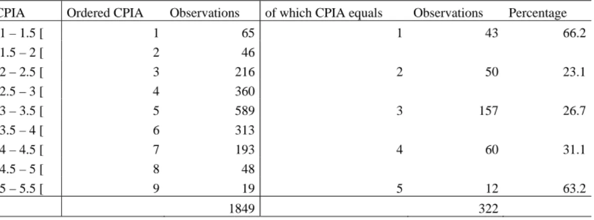
The CPIA is ordinal in nature. Each of its twenty components is rated on a scale from 1 to 6. Because it is an average of twenty components the CPIA can take all the values within this range, as illustrated by Table 1. Our core use of this ordinal variable is to create a dummy variable which takes the value of unity

ordered probit. Both of these approaches involve a loss of information. This is the price to be paid for respecting the ordinal nature of the variable: there is little sense in which an improvement from 2 to 3 is equivalent to an improvement from 3 to 4. However, the maximum potential information is to be achieved from ignoring these concerns and treating the CPIA as though it were cardinal. We therefore also investigate these variants, both in levels and in differences.

Table 1. Country Policy and Institutional Assessment, 1978-2004, 82 countries

CPIA Ordered CPIA Observations of which CPIA equals Observations Percentage

[1 – 1.5 [ 1 65 1 43 66.2 [1.5 – 2 [ 2 46 [2 – 2.5 [ 3 216 2 50 23.1 [2.5 – 3 [ 4 360 [3 – 3.5 [ 5 589 3 157 26.7 [3.5 – 4 [ 6 313 [4 – 4.5 [ 7 193 4 60 31.1 [4.5 – 5 [ 8 48 [5 – 5.5 [ 9 19 5 12 63.2 1849 322

In our cardinal treatment of the CPIA we first estimate a model of the following form:

, , 1 ', ', ,

i t i t i t i t i t i t

CPIA =CPIA ₋ +X

β

θ ϕ τ ε

where i (i = 1…N) denote countries and t (t = 1…T) denote years. Xi,t and Electioni,t are respectively a set

of control and election variables. ϕi and τt are respectively country fixed effects and years dummies.

The first way to estimate equation (1) is to use a Within estimator, which is asymptotically biased on finite

T (Nickell, 1981; Sevestre and Trognon, 1985). However, our sample is large (more than 1,000

observations) and the average T is 23 years (the maximum being 27 years), suggesting that the bias plaguing the Within estimator is close to zero (Judson and Owen, 1999). The second way of estimating equation (1) is to transform the model in first-difference. OLS estimations of the first-difference transformation of equation (1) may still be biased because of the correlation between the lagged endogenous variable and the error term. An alternative is to use the application of the Generalized Method of Moments proposed by Arellano and Bond (1991) and to instrument ∆CPIAi,t-1 by its lagged values in

level starting from t-2.

One of our ordinal strategies is to estimate an ordered probit model of the following form:

, 1 , , ,

*_{i t t} '_{i t} '_{i t i t i t}

CPIA =CPIA₋ +X

β

θ ϕ τ ε

where 1 , 2 2 , 3 , J , J+1 1 if < 2 if < * ... J if < i t i t i t i t CPIA CPIA CPIA CPIA µ µ µ µ µ µ ≤ ⎧ ⎪ _≤ ⎪ = ⎨ ⎪ ⎪ _≤ ⎩ .

The other ordinal strategy is to explain positive changes in the CPIA by means of a logit model of the following form:

, , ', ', ,

i t i t i t i t i t i t

Change =CPIA +X

β

θ ϕ τ ε

where _, , , 1 if 0 0 if 0 i t i t i t CPIA Change CPIA ∆ > ⎧⎪ = ⎨ _{∆ ≤} ⎪⎩ .

Because equation (3) links the changes in the CPIA to level variables it may omit some important control variables. Changes in the CPIA may be more related to changes in Xi,t than to the level of Xi,t. Equation

(3) can therefore be augmented in the following way:

, , ', ', ', ,

i t i t i t i t i t i t i t

Change =CPIA +X

β

γ

θ ϕ τ ε

Of the three empirical strategies, we use the third one as our core analysis and test its robustness using the two other strategies. The choice of one strategy over the other crucially depends on how ordinal the CPIA is considered to be. The advantage of the third strategy is to respect the ordinal nature of the CPIA without making any strong econometric assumptions as to the ordinality / cardinality of the CPIA.

Finally, the choice of the CPIA as our core dependent variable is crucial to our analysis, and as noted above is not without raising substantial conceptual and econometric issues. We therefore test the robustness of our baseline model using the ICRG (International Country Risk Guide). The ICRG is a rating of countries according to their economic and political environment, which reflects the feeling of private investors. The ICRG is an alternative measure of policy and institutions which gives more weigh than the CPIA to the quality of institutions (corruption, rule of law, quality of bureaucracy, etc.). As such, it is both an interesting robustness check and a good complement to our analysis using the CPIA. 3.2. Variables and Data

Policy and institutions depend on a set of control variables, Xi,t, and on a set of variables relating to

politics, Electioni,t. Xi,t include conventional development indicators: the level of income and its square,

population and education. It also includes more structural characteristics such as the share of the natural resource rents in GDP, and whether the country is at war. These variables and their sources are presented in detail in Appendix 2.

Electioni,t is a set of variables relating to the timing of elections. Data on elections are from the Database

on Political Institutions (DPI) of the World Bank. To test the robustness of our results, we also use the database on elections used by Brender and Drazen (2005) and provided by Allan Drazen. Since our analysis is based on annual observations elections that occur early in the year may be more appropriately assigned to the previous year. We discuss this issue more fully in Section 4.

Knowing election years we construct four variables to precisely capture the characteristics of the electoral timing and test the cyclical and structural effects of elections raised in section 2. The first one, FREQUENCY of election, is the number of years between the current election and the previous election. We lag this variable because of its potential endogeneity with respect to the chances of reform. By lagging, we mean that if an election occurs in year t, FREQUENCY is equal to the number of years between election in year t and the previous election. This number is reported for each year of the mandate starting in year t3.

To construct FREQUENCY, the country obviously needs to have held at least two elections. FREQUENCY is therefore equal to 0 if the country never had an election as well as during the mandate following the first elections. To control for this characteristic of FREQUENCY, we construct two dummy variables: NEVER, which is equal to 1 for the period during which the country never had an election – knowing that we have information on elections since 1975 –, and FIRST which is equal to one during the first mandate.

The fourth variable captures the political cycle. CYCLE is constructed as the number of years that separate year t from the nearest election, whether this is the previous election or the next election. So if an

3 _{We also reconstruct FREQUENCY of elections using Drazen’s database. This further allows us to tackle the endogeneity issue of the timing of} elections by distinguishing between predetermined and endogenous elections (see Section 5 on robustness checks).

election occurs in years t and t+4, CYCLE is equal to 0 in both years t and t+4; it is equal to 1 in years

t+1 and t+3 ; and it is equal to 2 in year t+2.

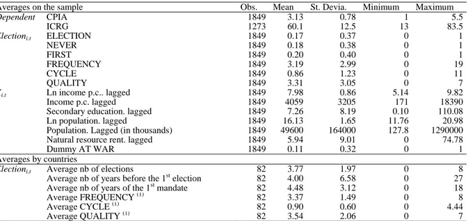
Table 2 provides some summary statistics on the dependent variables, on Xi,t and on the various variables

included in Electioni,t.

Table 2. Descriptive statistics, 1978-2004, 82 countries.

Averages on the sample Obs. Mean St. Devia. Minimum Maximum

Dependent CPIA 1849 3.13 0.78 1 5.5

ICRG 1273 60.1 12.5 13 83.5

Electioni.t ELECTION 1849 0.17 0.37 0 1

NEVER 1849 0.18 0.38 0 1

FIRST 1849 0.20 0.40 0 1

FREQUENCY 1849 3.19 2.99 0 19

CYCLE 1849 0.86 1.23 0 11

QUALITY 1849 3.31 3.05 0 7

Xi.t Ln income p.c.. lagged 1849 7.98 0.86 5.14 9.82

Income p.c. lagged 1849 4059 3205 171 18390 Secondary education. lagged 1849 7.26 8.19 0.10 110.08

Ln population. lagged 1849 16.13 1.65 11.76 20.98 Population. Lagged (in thousands) 1849 49600 164000 127.8 1290000

Natural resource rent. lagged 1849 5.94 9.01 0 74.78

Dummy AT WAR 1849 0.11 0.32 0 1

Averages by countries

Electioni.t Average nb of elections 82 3.77 1.97 0 8

Average nb of years before the 1st election 82 4.00 6.58 0 27 Average nb of years of the 1st mandate 82 4.48 3.12 0 18

Average FREQUENCY (1) _{82 3.37 1.49 0 8}

Average CYCLE (1) 82 0.90 0.60 0 4.44 Average QUALITY (1) 82 3.54 2.06 0 7 (1): calculated on the period following the first mandate. Our sample of 1849 observations contains 82 developing countries on a

period from 1978 to 2004. When we use the ICRG, this sample is reduced to 1273 observation on 70 countries on a period from 1985 to 2005.

4. ESTIMATION OF THE BASELINE MODEL

We now turn to our results. We investigate whether elections create pressures for better policies and governance on a sample of 82 developing countries on annual data from 1978 to 2004. A priori no single statistical approach dominates and so we present results using four different ones. Similarly, there are two distinct data sets on policy and governance, two data sets on elections, and potentially three different options for assigning elections to calendar years. Since the number of possible permutations of these options is considerable we proceed by presenting first a ‘core’ regression and then progressively introducing alternatives. While not all permutations are presented, all have been investigated and we note in the text those which are significantly different. Complete results are available from the authors.

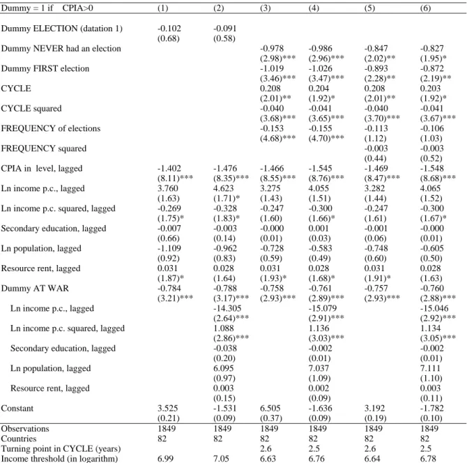
In Table 3 we explore the factors that lead to a year-on-year improvement in the CPIA. We estimate Equations (3) and (4). Since the CPIA is not a cardinal variable, we analyze its change by creating a dummy variable which takes the value of unity if it has improved relative to the previous year and estimate the probability of improvement through a logit regression. Subsequently we investigate a cardinal treatment of the CPIA.

Table 3. Logit estimations of the baseline model, 1978-2004, 82 countries.

Dummy = 1 if CPIA>0 (1) (2) (3) (4) (5) (6) Dummy ELECTION (datation 1) -0.102 -0.091

(0.68) (0.58)

Dummy NEVER had an election -0.978 -0.986 -0.847 -0.827

(2.98)*** (2.96)*** (2.02)** (1.95)*

Dummy FIRST election -1.019 -1.026 -0.893 -0.872

(3.46)*** (3.47)*** (2.28)** (2.19)** CYCLE 0.208 0.204 0.208 0.203 (2.01)** (1.92)* (2.01)** (1.92)* CYCLE squared -0.040 -0.041 -0.040 -0.041 (3.68)*** (3.65)*** (3.70)*** (3.67)*** FREQUENCY of elections -0.153 -0.155 -0.113 -0.106 (4.68)*** (4.70)*** (1.12) (1.03) FREQUENCY squared -0.003 -0.003 (0.44) (0.52)

CPIA in level, lagged -1.402 -1.476 -1.466 -1.545 -1.469 -1.548 (8.11)*** (8.35)*** (8.55)*** (8.76)*** (8.47)*** (8.68)*** Ln income p.c., lagged 3.760 4.623 3.275 4.055 3.282 4.065

(1.63) (1.71)* (1.43) (1.51) (1.44) (1.52) Ln income p.c. squared, lagged -0.269 -0.328 -0.247 -0.300 -0.247 -0.300 (1.75)* (1.83)* (1.60) (1.66)* (1.61) (1.67)* Secondary education, lagged -0.007 -0.003 -0.000 0.001 -0.001 -0.000

(0.66) (0.14) (0.01) (0.03) (0.06) (0.01) Ln population, lagged -1.109 -0.962 -0.728 -0.583 -0.748 -0.605

(0.92) (0.83) (0.59) (0.49) (0.60) (0.50) Resource rent, lagged 0.031 0.028 0.031 0.028 0.031 0.028 (1.87)* (1.64) (1.93)* (1.68)* (1.91)* (1.63) Dummy AT WAR -0.784 -0.788 -0.758 -0.761 -0.757 -0.760 (3.21)*** (3.17)*** (2.93)*** (2.89)*** (2.93)*** (2.88)***

Ln income p.c., lagged -14.305 -15.079 -15.046

(2.64)*** (2.91)*** (2.92)***

Ln income p.c. squared, lagged 1.088 1.136 1.134

(2.86)*** (3.03)*** (3.05)***

Secondary education, lagged -0.038 -0.002 -0.002

(0.20) (0.01) (0.01)

Ln population, lagged 6.095 7.037 7.111

(0.97) (1.09) (1.10)

Resource rent, lagged 0.003 0.002 0.003

(0.15) (0.09) (0.11)

Constant 3.525 -1.531 6.505 -1.636 3.192 -1.782 (0.21) (0.09) (0.37) (0.09) (0.19) (0.10) Observations 1849 1849 1849 1849 1849 1849

Countries 82 82 82 82 82 82

Turning point in CYCLE (years) 2.6 2.5 2.6 2.5

Income threshold (in logarithm) 6.99 7.05 6.63 6.76 6.64 6.78 Robust z statistics in parentheses. Standard errors are adjusted for intra-country correlation. * significant at 10%; ** significant at 5%; *** significant at 1%.

DEPENDENT VARIABLE: Dummy = 1 when CPIA is strictly positive. ESTIMATION METHOD: Logit with country fixed effects and year dummies.

DATING OF ELECTIONS: The electoral dummy equals one in an election year and zero otherwise, no matter when during the year the election occurred. NEVER, FIRST, CYCLE and FREQUENCY are constructed according to this dating of elections.

The first two columns provide baseline logit regressions with fixed effects and year dummies. Elections are introduced in the simplest possible form, namely a dummy variable which takes the value of unity if there is an election during the year. As with the other regressions in this table the election is assigned to the calendar year in which it occurs. The other explanatory variables are the CPIA, income and its square, secondary education, the size of the population, and the value of natural resource rents, all these variables being lagged. A dummy variable takes the value of unity if the country is at war. The regression in column (1) only the levels of these explanatory variables are included, whereas in (2) the changes in these variables are included along with their levels.

In both regressions the dummy variable for elections is completely insignificant. Elections, the key institutional technology of democracy, appear to wash over the society without affecting economic policy. However, as we will show, this result is spurious and misleading. It may compound offsetting cyclical and structural effects, or it may reflect endogeneity. The better is the CPIA the harder it is to improve it further, the result being highly significant in both regressions. Per capita income has non-linear effects that are borderline significant: reform is most likely at around $1150 per capita. Out of the 82 countries in our sample, only 17 have a per capita income lower than this threshold, all but Nepal in Africa. Low income thus appears to be a stimulus to change. Somewhat surprisingly, natural resource rents have positive effects that are borderline significant. This may appear to run counter to the resource curse literature. However, that literature is concerned with the long term effects and the short term effects may be benign. Unsurprisingly, civil wars have a significantly negative impact on the probability that policy and institutions will improve. Annual time dummies (not reported) suggest that policies are getting better over time. While this may reflect nothing more than grade inflation on the part of World Bank staff, it is reasonable to expect that in countries which mostly only became independent during the 1960s governments would go through a gradual learning process.

The regressions of columns 3 and 4 introduce the variables that are consistent with the discussion of theory in Section 2. Four new variables between them characterize elections. As discussed in Section 3, one is a dummy variable characterizing countries which up to the year being considered have never had an election during the period 1978-2004. A second is a dummy variable for those observations in which there has been only one prior election in the country. The third variable – CYCLE – is the time in the electoral cycle as measured by the number of years that separate the year in question from the nearest election, whether this is the previous election or the next election. Note that this conflates two potentially distinct distances: forward-looking and backward-looking. Thus, in this regression we treat the shortening horizon effect and the populist legacy effect as symmetrical. In subsequent analysis we test whether this conflation is warranted on the data. Both CYCLE and its square are included. As discussed in Section 2, the effect of the time from the nearest election is unlikely to be monotonic. While in the vicinity of the election greater distance from it might improve policy, if the nearest election is very distant then the accountability of government to the electorate may be weakened. The final new variable – FREQUENCY – captures the frequency of elections. It is measured by the length of time between the most recent previous election and the one prior to that. Hence, the higher is the value of the variable the less frequent are elections.

The control variables are the same as in the first two regressions. The regression of column (3) includes only the levels of these variables whereas that of column (4) also includes their changes. As previously, all these variables are lagged. The introduction of the new variables for elections does not significantly change the coefficients or significant levels of these control variables and so we focus on the election variables themselves.

In contrast to the naïve approach of columns (1) and (2), all the elections variables are now significant. The inclusion of the changes in the control variables in addition to their levels makes virtually no difference to either coefficients or significance levels, nearly all of which are at one percent. What do the coefficients imply?

The dummy for those countries which never held an election prior to the year under observation has a large negative coefficient. This is consistent with the hypothesis that elections introduce accountability, although the interpretation need not be causal. An alternative interpretation is that the absence of elections is a symptom of a more fundamental problem that prevents improvements in economic policy and governance rather than being its explanation. However, in addition to the control variables, recall that this regression includes fixed effects so that for all countries which did not have an election over the entire period 1978-2004 any effects of the absence of elections are subsumed in the fixed effect. Essentially, the variable NEVER is picking up the difference between periods prior to the first election and those

and negative, and statistically indistinguishable from that on the dummy for countries that never held elections. The most reasonable interpretation is that a single election is insufficient to change the behaviour of a government.

The remaining three variables, CYCLE, its square, and FREQUENCY, exclude the first election. We start with FREQUENCY which is the structural relationship. Recall that the variable measures the number of years between the two previous elections. Hence, an increase in the variable is a reduction in the frequency of elections. The negative coefficient therefore implies that the more frequent are elections the more likely is the CPIA to improve. This is consistent with the accountability and legitimacy theory of democracy. As with the two dummy variables for countries which have never held elections or have only held one, the frequency of elections may itself proxy some characteristics not included in our control variables, but the deep and unchanging characteristics are all subsumed by means of fixed effects.

Taken together with the negative and highly significant coefficients on the dummy variables, the negative and highly significant coefficient on FREQUENCY suggests that sustained elections really do have a structural effect on economic policy and governance, over the observed period increasing the chance of policy improvement and presumably in the long run improving the level of policy. Despite the reasons to fear that in developing countries governments might be able to win elections without regard to policy, democracy appears to work.

We now turn to CYCLE and its square. Both are significant, and whereas if the squared term is excluded CYCLE itself loses significance. CYCLE is positive and its square is negative: what does this mean? Recall that CYCLE measures the time until the nearest election, either viewed back to the previous one or forward to the next. An important issue is going to be whether this conflation of effects is warranted on the data, but for the moment we will focus on what it implies if it is warranted. The positive coefficient on CYCLE implies that the further away is an election the better are the chances of policy reform. This indicates a tension between elections as important structural instruments of democracy and as periodic events which interrupt the normal business of government. Because both effects matter, any measure which conflates them is liable to be misleading. The negative coefficient on the square of CYCLE indicates that as the distance from an election increases at some point the benefits of further distance are exhausted and go into reverse. Since FREQUENCY is included, the periodicity of elections is already controlled for. However, it implies that if the periodicity is infrequent then the mid-term is not a good time for policy reform. This becomes clearest if elections are very infrequent, such as once-a-decade. In such a case it is indeed plausible that at the mid-term the government would be less conscious of accountability to citizens.

The socially optimal periodicity of elections implied by these results depends upon the three variables in combination. This is explored further in Section 7. However, here we pose a seemingly simple question: if elections increase accountability can elections be too frequent? As the periodicity is increased there are opposing effects. The direct effect of an increased value of FREQUENCY is adverse. However, a longer periodicity also changes the average composition of the years within each period: proportionately less time is very close to an election. Up to a point, this effect is benign. Hence, for the social optimum the net effect must be calculated and this is taken up in Section 7.

The inclusion of the square of CYCLE but not the square of FREQUENCY may appear arbitrary. We first provide a degree of reassurance by adding the square of FREQUENCY in columns (5) and (6): the square is insignificant. There is indeed a good reason other than this result for the core regression to take the form of (3) and (4). Given that the structural and cyclical effects of elections are qualitatively offsetting, the minimum specification that can hope to capture optimality must include at least one squared term (or adopt some other function form which allows non-linearity). If, as appears to be the case, as periodicity is increased beyond a point the chances of reform in the mid-term period deteriorate, this can be captured better by including the square of CYCLE than the square of FREQUENCY. However, to include the square of both terms would build in redundancy.

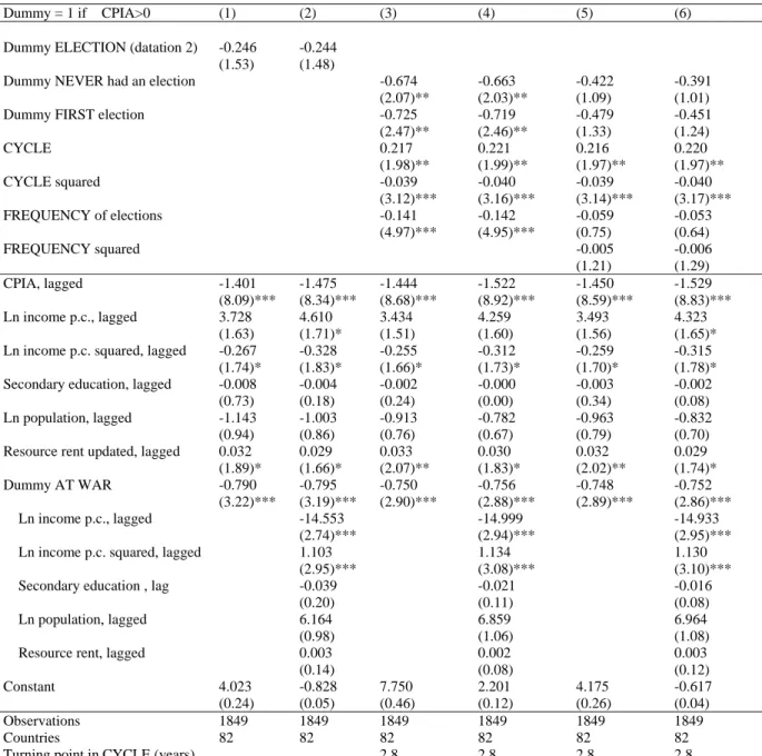
A fundamental aspect of the variable CYCLE is that it combines the backward and forward-looking effects of elections. In Tables 4 and 5 we investigate whether this is warranted. The conventional political economy analysis of elections is forward-looking: as the election approaches the government is less inclined to invest in policy reform because a higher proportion of the benefits will accrue after the election. If this is the only effect of elections on policy then an implication is that if analysis is based on annual observations those elections that occur in the first half of the year should be reassigned to the previous year. For example, almost all of the effects of an election held in January will be on policy decisions in the previous year. We now investigate whether such reassignment is superior to the strategy adopted in Table 3. In Table 4 we introduce dummy variables according to whether the election is in the first or second half of the year and interact them with the election variables. The key new variables are the interactions with CYCLE and its square. Evidently, since the cyclical effects are now spread over four variables instead of two, each pair with only around half as many observations, we might expect some loss of significance. However, the loss of significance is considerably more severe for the elections occurring in the first half of the year than in the second. This result suggests that the forward-looking effect of elections may be the only one of importance in which case the dating of elections should be changed accordingly. In Table 5 we therefore re-run the regressions of Table 3 but with the revised dating and compare it with Table 3. There is little to choose between the two sets of regressions. On the criterion of the p-values of the two cyclical variables judged on the two core regressions of columns (3) and (4) the original dating slightly outperforms: three of the four p-values are higher. On the criterion of the other election variables the preference for the original dating is a little stronger: in particular, the p-values on the two election dummy variables drop considerably with when elections in the first half of the year are re-assigned to the previous year. Fortunately, the actual coefficients on the election variables are virtually unaltered. We therefore retain the calendar dating of elections, thereby implicitly giving legacy effects similar weight to anticipation effects. Quite possibly the anticipation effects are stronger than the legacy effects but not the entire story.

Table 4. Baseline model, splitting the timing of elections, 1978-2004, 82 countries.

Dummy = 1 if CPIA>0 (1) (2) (3) (4) (5) (6) Dummy NEVER had an election -1.159 -1.169 -0.970 -0.949

(3.44)*** (3.43)*** (2.21)** (2.13)**

Variables in interaction with a dummy FIRST HALF of the year Dummy ELECTION 0.044 0.068

(0.21) (0.32)

Dummy FIRST election -0.868 -0.871 -0.691 -0.665

(2.85)*** (2.87)*** (1.64) (1.56) CYCLE -0.008 -0.036 0.021 -0.008 (0.03) (0.16) (0.09) (0.03) CYCLE squared 0.073 0.075 0.067 0.069 (0.95) (1.01) (0.89) (0.95) FREQUENCY of elections -0.149 -0.150 -0.114 -0.105 (4.16)*** (4.13)*** (1.12) (1.00) FREQUENCY squared -0.001 -0.002 (0.25) (0.34)

Variables in interaction with a dummy SECOND HALF of the year Dummy ELECTION -0.250 -0.252

(1.09) (1.06)

Dummy FIRST election -1.506 -1.522 -1.315 -1.297 (4.05)*** (4.03)*** (2.79)*** (2.67)*** CYCLE 0.143 0.154 0.128 0.139 (1.01) (1.06) (0.87) (0.92) CYCLE squared -0.038 -0.041 -0.037 -0.039 (2.69)*** (2.83)*** (2.52)** (2.66)*** FREQUENCY of elections -0.206 -0.211 -0.120 -0.113 (4.25)*** (4.33)*** (0.83) (0.77) FREQUENCY squared -0.008 -0.009 (0.70) (0.76)

CPIA in level, lagged -1.402 -1.477 -1.489 -1.564 -1.491 -1.566

(8.09)*** (8.33)*** (8.66)*** (8.88)*** (8.63)*** (8.84)*** Ln income p.c., lagged 3.774 4.650 3.002 3.862 2.962 3.800

(1.65)* (1.73)* (1.31) (1.44) (1.31) (1.43) Ln income p.c. squared, lagged -0.270 -0.331 -0.228 -0.287 -0.226 -0.284

(1.77)* (1.84)* (1.48) (1.58) (1.48) (1.58) Secondary education, lagged -0.006 -0.003 0.000 0.004 -0.001 0.002 (0.63) (0.13) (0.05) (0.17) (0.06) (0.10) Ln population, lagged -1.126 -0.985 -0.764 -0.627 -0.836 -0.702 (0.93) (0.84) (0.61) (0.52) (0.65) (0.57) Resource rent, lagged 0.032 0.028 0.035 0.032 0.034 0.032

(1.87)* (1.65)* (2.22)** (2.01)** (2.19)** (1.95)* Dummy AT WAR -0.792 -0.798 -0.772 -0.779 -0.775 -0.779

(3.22)*** (3.19)*** (2.89)*** (2.90)*** (2.90)*** (2.90)*** Ln income p.c., lagged -14.576 -14.972 -14.569

(2.74)*** (2.87)*** (2.84)***

Ln income p.c. squared, lagged 1.107 1.124 1.100

(2.96)*** (2.99)*** (2.97)***

Secondary education, lagged -0.037 -0.031 -0.027

(0.19) (0.16) (0.14)

Ln population, lagged 6.098 7.164 7.453

(0.97) (1.06) (1.08)

Resource rent, lagged 0.003 0.002 0.003

(0.14) (0.07) (0.12)

Observations (countries) 1849 (82) 1849 (82) 1849 (82) 1849 (82) 1849 (82) 1849 (82) Robust z statistics in parentheses. Standard errors are adjusted for intra-country correlation. * significant at 10%; ** significant at 5%; *** significant at 1%. DEPENDENT VARIABLE: Dummy = 1 when CPIA is strictly positive. ESTIMATION METHOD: Logit with country fixed effects and year dummies, constant included but not shown. DATING OF ELECTIONS: The electoral dummy equals one in an election year and zero otherwise, no matter when during the year the election occurred. NEVER, FIRST, CYCLE and FREQUENCY are constructed according to this dating of elections. The dummies FIRST and SECOND half of the year are equal to one if the elections were held, respectively, before and after June. This dummy is equal to one during the whole duration of the mandate.

Table 5. Baseline model, alternative dating of elections, 1978-2004, 82 countries.

Dummy = 1 if CPIA>0 (1) (2) (3) (4) (5) (6) Dummy ELECTION (datation 2) -0.246 -0.244

(1.53) (1.48)

Dummy NEVER had an election -0.674 -0.663 -0.422 -0.391 (2.07)** (2.03)** (1.09) (1.01) Dummy FIRST election -0.725 -0.719 -0.479 -0.451

(2.47)** (2.46)** (1.33) (1.24) CYCLE 0.217 0.221 0.216 0.220 (1.98)** (1.99)** (1.97)** (1.97)** CYCLE squared -0.039 -0.040 -0.039 -0.040 (3.12)*** (3.16)*** (3.14)*** (3.17)*** FREQUENCY of elections -0.141 -0.142 -0.059 -0.053 (4.97)*** (4.95)*** (0.75) (0.64) FREQUENCY squared -0.005 -0.006 (1.21) (1.29) CPIA, lagged -1.401 -1.475 -1.444 -1.522 -1.450 -1.529 (8.09)*** (8.34)*** (8.68)*** (8.92)*** (8.59)*** (8.83)*** Ln income p.c., lagged 3.728 4.610 3.434 4.259 3.493 4.323 (1.63) (1.71)* (1.51) (1.60) (1.56) (1.65)* Ln income p.c. squared, lagged -0.267 -0.328 -0.255 -0.312 -0.259 -0.315

(1.74)* (1.83)* (1.66)* (1.73)* (1.70)* (1.78)* Secondary education, lagged -0.008 -0.004 -0.002 -0.000 -0.003 -0.002

(0.73) (0.18) (0.24) (0.00) (0.34) (0.08) Ln population, lagged -1.143 -1.003 -0.913 -0.782 -0.963 -0.832

(0.94) (0.86) (0.76) (0.67) (0.79) (0.70) Resource rent updated, lagged 0.032 0.029 0.033 0.030 0.032 0.029

(1.89)* (1.66)* (2.07)** (1.83)* (2.02)** (1.74)* Dummy AT WAR -0.790 -0.795 -0.750 -0.756 -0.748 -0.752 (3.22)*** (3.19)*** (2.90)*** (2.88)*** (2.89)*** (2.86)***

Ln income p.c., lagged -14.553 -14.999 -14.933

(2.74)*** (2.94)*** (2.95)*** Ln income p.c. squared, lagged 1.103 1.134 1.130

(2.95)*** (3.08)*** (3.10)*** Secondary education , lag -0.039 -0.021 -0.016

(0.20) (0.11) (0.08) Ln population, lagged 6.164 6.859 6.964

(0.98) (1.06) (1.08) Resource rent, lagged 0.003 0.002 0.003

(0.14) (0.08) (0.12)

Constant 4.023 -0.828 7.750 2.201 4.175 -0.617 (0.24) (0.05) (0.46) (0.12) (0.26) (0.04) Observations 1849 1849 1849 1849 1849 1849

Countries 82 82 82 82 82 82

Turning point in CYCLE (years) 2.8 2.8 2.8 2.8

Robust z statistics in parentheses. Standard errors are adjusted for intra-country correlation. * significant at 10%; ** significant at 5%; *** significant at 1%.

DEPENDENT VARIABLE: Dummy = 1 when ∆ CPIA is strictly positive. ESTIMATION METHOD: Logit with country fixed effects and year dummies.

SECOND DATING: The electoral dummy equals one in an election year if the election occurs after June and in the year before the election year it the election occurs before June. It is equal to zero otherwise. NEVER, FIRST, CYCLE and FREQUENCY are constructed according to this dating of elections.

information by treating the CPIA as ordinal. Our second set of robustness checks therefore explores alternative estimation methods using equations (1) and (2). A third set of robustness checks provides estimations of our baseline model using Allan Drazen’s database of elections. Using this dataset also allows to explore the potential endogeneity issue of our elections variables by distinguishing between constitutionally predetermined elections and endogenous elections. Finally, our fourth set of robustness checks focuses more specifically on the CYCLE variable and proposes alternative ways of measuring political cycles.

5.1. Estimations using the ICRG

Our first variant on these core results is to switch from the CPIA as a measure of policy improvement to the ICRG rating. Recall that the ICRG is a commercial rating and so is subject to the discipline of the market. However, it covers fewer countries that the World Bank rating and only a period starting in 1985.4 Further, as the recent travails of the credit rating agencies indicate, the discipline of the market may in practice produce worse quality than that of an impartial public bureaucracy.

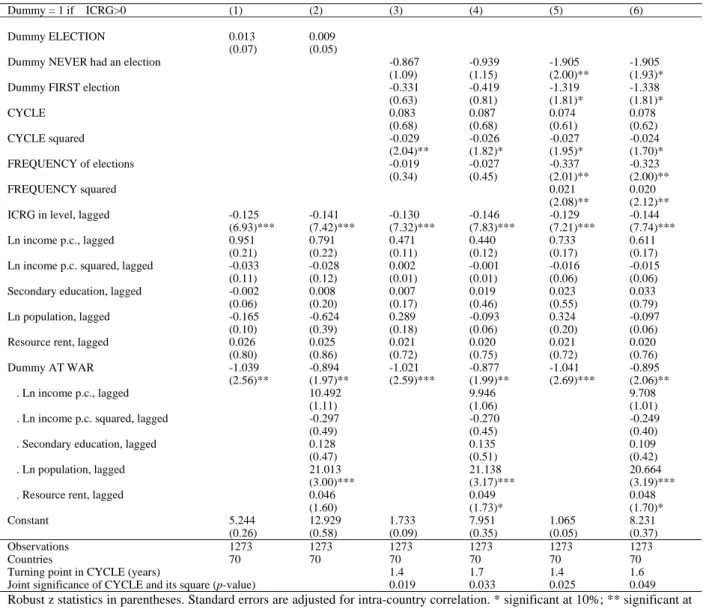
Table 6 reproduces the regressions of Table 3 with the dependent variable being a dummy which is equal to one when changes in the ICRG are positive. Among the control variables, it agrees with the World Bank data in finding that there has been an improvement in policy year-by-year that is unrelated to the other explanatory variables (the time dummies are not shown in the Table). Hence, our former result is unlikely to be fully explained by grade inflation among World Bank staff. The result is important because it severs the secular improvement in policy from the spread of democracy.

As to our election variables, it finds the same cyclical and structural effects as using the CPIA data. Although CYCLE is not individually significant its square is and so the two variables should be assessed in terms of their joint significance. The last row of Table 6 reports that CYCLE and its square are jointly significant at 5%.

The ICRG gives more weight to institutions – rule of law, corruption, quality of bureaucracy, etc. – than the CPIA which is primarily focused on economic policy and structural economic reforms. A minor difference between Tables 3 and 6 is that FREQUENCY only becomes significantly negative once its square is introduced. Although the squared term is positive, within the relevant range of the data it almost never predominates. The turning point is in excess of 8 years which is found only in Liberia, Sierra Leone and Togo. The results are thus consistent with those of Table 3.

Finally, NEVER and FIRST have the same negative coefficient as in Table 3, but are less robustly significant.

4

Three countries are in the ICRG database but not in the CPIA one: Barhain, Iran and Iraq. We ran the estimations with and without these countries and it did not change our results. Moreover, the ICRG is available for more recent years than the CPIA. Therefore Table 6 covers 2005, while Table 3 stopped in 2004.

Table 6. Robustness checks using ICRG, 1985-2005, 70 countries.

Dummy = 1 if ICRG>0 (1) (2) (3) (4) (5) (6)

Dummy ELECTION 0.013 0.009

(0.07) (0.05)

Dummy NEVER had an election -0.867 -0.939 -1.905 -1.905

(1.09) (1.15) (2.00)** (1.93)*

Dummy FIRST election -0.331 -0.419 -1.319 -1.338

(0.63) (0.81) (1.81)* (1.81)* CYCLE 0.083 0.087 0.074 0.078 (0.68) (0.68) (0.61) (0.62) CYCLE squared -0.029 -0.026 -0.027 -0.024 (2.04)** (1.82)* (1.95)* (1.70)* FREQUENCY of elections -0.019 -0.027 -0.337 -0.323 (0.34) (0.45) (2.01)** (2.00)** FREQUENCY squared 0.021 0.020 (2.08)** (2.12)**

ICRG in level, lagged -0.125 -0.141 -0.130 -0.146 -0.129 -0.144

(6.93)*** (7.42)*** (7.32)*** (7.83)*** (7.21)*** (7.74)*** Ln income p.c., lagged 0.951 0.791 0.471 0.440 0.733 0.611

(0.21) (0.22) (0.11) (0.12) (0.17) (0.17) Ln income p.c. squared, lagged -0.033 -0.028 0.002 -0.001 -0.016 -0.015

(0.11) (0.12) (0.01) (0.01) (0.06) (0.06) Secondary education, lagged -0.002 0.008 0.007 0.019 0.023 0.033 (0.06) (0.20) (0.17) (0.46) (0.55) (0.79) Ln population, lagged -0.165 -0.624 0.289 -0.093 0.324 -0.097

(0.10) (0.39) (0.18) (0.06) (0.20) (0.06) Resource rent, lagged 0.026 0.025 0.021 0.020 0.021 0.020 (0.80) (0.86) (0.72) (0.75) (0.72) (0.76) Dummy AT WAR -1.039 -0.894 -1.021 -0.877 -1.041 -0.895

(2.56)** (1.97)** (2.59)*** (1.99)** (2.69)*** (2.06)**

. Ln income p.c., lagged 10.492 9.946 9.708

(1.11) (1.06) (1.01)

. Ln income p.c. squared, lagged -0.297 -0.270 -0.249

(0.49) (0.45) (0.40)

. Secondary education, lagged 0.128 0.135 0.109

(0.47) (0.51) (0.42)

. Ln population, lagged 21.013 21.138 20.664

(3.00)*** (3.17)*** (3.19)***

. Resource rent, lagged 0.046 0.049 0.048

(1.60) (1.73)* (1.70)*

Constant 5.244 12.929 1.733 7.951 1.065 8.231

(0.26) (0.58) (0.09) (0.35) (0.05) (0.37)

Observations 1273 1273 1273 1273 1273 1273

Countries 70 70 70 70 70 70

Turning point in CYCLE (years) 1.4 1.7 1.4 1.6

Joint significance of CYCLE and its square (p-value) 0.019 0.033 0.025 0.049 Robust z statistics in parentheses. Standard errors are adjusted for intra-country correlation. * significant at 10%; ** significant at 5%; *** significant at 1%.

DEPENDENT VARIABLE: Dummy = 1 when ∆ ICRG is strictly positive. ESTIMATION METHOD: Logit with country fixed effects and year dummies.

DATING OF ELECTIONS: The electoral dummy equals one in an election year and zero otherwise, no matter when during the year the election occurred. NEVER, FIRST, CYCLE and FREQUENCY are constructed according to this dating of elections.

5.2. Robustness of the estimation method: estimation of equations (1) and (2)

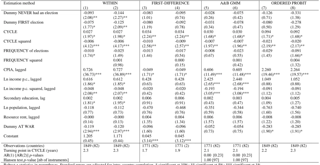
We next turn to robustness checks of the estimation method. More specifically, Table 7 presents the estimations of Equation (1) – assuming continuous CPIA – using three different estimation methods: within estimator, OLS on first-difference, and Arellano and Bond (1991) GMM estimator. It also presents the estimations of Equation (2) – assuming ordered CPIA – using an ordered probit model.

These results are presented in Table 7. The most striking result is the robustness of the CYCLE effect. In Table 7, the turning point is relatively stable, between 1.7 and 2.3, and close to that of Table 3. The coefficients on FREQUENCY, NEVER and FIRST are all always negative, as in Table 3, but they are

Table 7. Robustness checks of the estimation method, 1978-2004, 82 countries.

Estimation method WITHIN FIRST-DIFFERENCE A&B GMM ORDERED PROBIT

(1) (2) (3) (4) (5) (6) (7) (8)

Dummy NEVER had an election -0.093 -0.144 -0.083 -0.095 -0.028 -0.075 -0.126 -0.331

(2.08)** (2.27)** (1.01) (0.74) (0.26) (0.42) (0.71) (1.38)

Dummy FIRST election -0.075 -0.125 -0.080 -0.092 -0.031 -0.078 -0.080 -0.278

(1.77)* (2.09)** (1.19) (0.78) (0.34) (0.47) (0.50) (1.29) CYCLE 0.027 0.027 0.034 0.034 0.030 0.030 0.094 0.092 (1.97)* (1.98)* (2.24)** (2.24)** (1.68)* (1.68)* (1.71)* (1.68)* CYCLE squared -0.006 -0.006 -0.010 -0.009 -0.007 -0.007 -0.021 -0.020 (4.12)*** (4.17)*** (2.58)** (2.57)** (1.97)** (1.96)** (2.19)** (2.17)** FREQUENCY of elections -0.010 -0.025 -0.013 -0.017 -0.008 -0.023 -0.029 -0.091 (1.74)* (1.49) (1.44) (0.54) (0.67) (0.55) (1.45) (1.66)* FREQUENCY squared 0.001 0.000 0.001 0.004 (0.98) (0.15) (0.42) (1.32) CPIA, lagged 0.726 0.727 -0.049 -0.049 0.606 0.605 2.260 2.264 (36.73)*** (36.89)*** (1.71)* (1.71)* (11.49)*** (11.48)*** (19.46)*** (19.57)*** Ln income p.c., lagged 0.616 0.612 0.428 0.428 2.425 2.440 1.049 1.052 (1.86)* (1.85)* (0.63) (0.63) (2.65)*** (2.68)*** (0.88) (0.88)

Ln income p.c. squared, lagged -0.048 -0.048 -0.020 -0.020 -0.193 -0.194 -0.091 -0.091

(2.08)** (2.07)** (0.42) (0.42) (3.05)*** (3.08)*** (1.12) (1.12)

Secondary education, lag 0.002 0.002 0.006 0.006 0.002 0.003 0.004 0.005

(1.81)* (1.95)* (0.91) (0.91) (0.43) (0.47) (1.09) (1.27)

Ln population, lagged -0.118 -0.112 -0.470 -0.468 -0.351 -0.344 -0.763 -0.740

(0.77) (0.73) (0.76) (0.76) (0.59) (0.58) (1.60) (1.56)

Resource rent, lagged -0.000 -0.000 0.004 0.004 0.006 0.006 -0.008 -0.008

(0.14) (0.13) (1.35) (1.34) (1.57) (1.57) (1.22) (1.20) Dummy AT WAR -0.119 -0.120 -0.096 -0.096 -0.052 -0.054 -0.283 -0.285 (2.94)*** (2.97)*** (1.60) (1.60) (0.73) (0.75) (1.90)* (1.91)* Constant 1.205 1.171 0.045 0.045 (0.45) (0.44) (3.14)*** (3.12)*** Observations (countries) 1849 (82) 1849 (82) 1771 (82) 1771 (2) 1771 (82) 1771 (82) 1849 (82) 1849 (82)

Turning point in CYCLE (years) 2.3 2.3 1.7 1.9 2.1 2.1 2.2 2.3

AR(1) [AR(2)] p-values 0.00 [0.23] 0.00 [0.23]

Hansen test p-value [nb of instruments] 1.00 [97] 1.00 [97]

Robust z statistics in parentheses. Standard errors are adjusted for intra-country correlation. * significant at 10%; ** significant at 5%; *** significant at 1%. Columns (1) and (2): Within estimations of equation (1); dependent variable is continuous CPIA; estimations include year dummies.

Columns (3) and (4): Estimations in first-difference of equation (1); dependent variable is continuous CPIA; estimations include year dummies.

Columns (5) and (6): Arellano and Bond GMM estimation of equation (1) transformed in first-difference; dependent variable is continuous CPIA; estimations include year dummies; two-step estimator, using levels of CPIA from t-2 to t-4 as instruments for CPIAi,t-1.

Columns (7) and (8): Estimation of ordered probit; the CPIA is ordered from 1 to 9 every 0.5 increment in the CPIA: estimations include year and country dummies.

Dating of elections: The electoral dummy equals one in an election year and zero otherwise, no matter when during the year the election occurred. NEVER, FIRST, CYCLE and FREQUENCY are constructed according to this dating of elections.