HAL Id: tel-00441654
https://pastel.archives-ouvertes.fr/tel-00441654
Submitted on 16 Dec 2009
HAL is a multi-disciplinary open access archive for the deposit and dissemination of sci-entific research documents, whether they are pub-lished or not. The documents may come from teaching and research institutions in France or abroad, or from public or private research centers.
L’archive ouverte pluridisciplinaire HAL, est destinée au dépôt et à la diffusion de documents scientifiques de niveau recherche, publiés ou non, émanant des établissements d’enseignement et de recherche français ou étrangers, des laboratoires publics ou privés.
metastable helium: fermion antibunching and a study of
boson pair correlations in the collision of two
condensates
Valentina Krachmalnicoff
To cite this version:
Valentina Krachmalnicoff. Two experiments on quantum correlations in gases of metastable helium: fermion antibunching and a study of boson pair correlations in the collision of two condensates. Atomic Physics [physics.atom-ph]. Université Paris Sud - Paris XI, 2009. English. �tel-00441654�
LABORATOIRE CHARLES FABRY DE L’INSTITUT D’OPTIQUE
UNIVERSITE PARIS XI
U.F.R. SCIENTIFIQUE D’ORSAY
THESE
présentée pour obtenir
le GRADE DE DOCTEUR EN SCIENCES
DE L’UNIVERSITE PARIS XI
par
Valentina KRACHMALNICOFF
Sujet:
DEUX EXPERIENCES DE CORRELATIONS QUANTIQUES
SUR DES GAZ DE HELIUM METASTABLE :
DEGROUPEMENT DE FERMIONS ET ETUDE DE PAIRES DE BOSONS
CORRELES PAR COLLISION DE CONDENSATS
Soutenue le 22 Juin 2009 devant le jury composé de :
Mr. C. WESTBROOK Directeur de thèse
Mr. J. DALIBARD Rapporteur
Mme H. PERRIN Rapporteur
Mr. P. GRANGIER Examinateur
Mr. M. INGUSCIO Examinateur
Mr. A. ASPECT Membre invité
Remerciements
Ces travaux de th`ese se sont d´eroul´es au Laboratoire Charles Fabry de l’Institut d’Optique. Je remercie son directeur Pierre Chavel de m’y avoir accueilli et d’avoir suivi avec int´erˆet mon travail de recherche tout au long de mon doctorat.
Je remercie de tout coeur le directeur du groupe d’Otique Atomique Alain Aspect, mon directeur de th`ese Chris Westbrook et le responsable de l’´equipe H´elium Denis Boiron pour m’avoir donn´e la possibilit´e de vivre cette exp´erience tr`es enrichissante, non seulement du point de vue scientifique mais aussi du pont de vue humain. J’ai eu la chance de pouvoir appr´ecier `a plusieurs reprises les qualit´es p´edagogiques d’Alain, lors des r´eunions de groupe, quand il se soucie que les “plus jeunes” du groupe comprennent les discussions, et lors de la redaction d’articles, quand il a plusieurs fois contribu´e `a clarifier des id´ees qui ´etaient encore embrouill´ees dans ma tˆete. Je le remercie aussi pour le soutien et les pr´ecieux conseils qu’il a su me donner lors du choix de mon post-doc.
D`es ma premi`ere visite `a l’Institut d’Optique, j’ai ´et´e frapp´ee par l’enthousiasme de Chris et par sa curiosit´e, qui ne s’arrˆete devant rien. Les nombreuses discussions sur les manips en cours et sur les manips futures, l`a o`u on peut voyager avec la cr´eativit´e et la fantaisie, sans pour cela oublier la physique, d´emontrent sa fraˆıcheur d’esprit dont j’esp`ere m’inspirer dans la suite. Je remercie aussi Chris pour m’avoir transmis son optimisme lors des moments difficiles : quand les caprices de la manip semblaient insur-montables ou quand rien ne semblait marcher selon le plan rationnel qu’on s’attendrait, tr`es na¨ıvement, devoir guider une exp´erience de physique.
Je remercie Denis pour la rigueur, la constance et la patience qu’il a d´emontr´e tous les jours et en toute occasion. J’ai toujours ´et´e pleine d’admiration pour sa capacit´e `
a r´epondre `a toutes les questions des th´esards (sans jamais se scandaliser ni pour leur na¨ıvet´e ni par le fait que la question lui avait d´ej`a ´et´e pos´ee auparavant!) et pour la grande clart´e de ses explications. De plus sa pr´esence quotidienne en salle de manip, sa capacit´e `a rester calme et `a rire aussi des situations qui semblent d´esesp´er´ees, ont ´et´e d’une grande aide pendant toute ma th`ese. Je le remercie aussi de tout coeur pour ses nombreuses relectures du manuscrit.
H´el`ene Perrin et Jean Dalibard ont eu la gentillesse d’accepter de rapporter cette th`ese. Je les remercie pour le vif int´erˆet qu’ils ont montr´e envers mon travail ainsi que pour leurs remarques int´eressantes sur le manuscrit, qui ont constitu´e un moment important de r´eflexion. Je remercie ´egalement Philippe Grangier pour l’enthousiasme
avec lequel il a accept´e d’ˆetre pr´esident du jury. Massimo Inguscio a fait partie du jury en tant que examinateur. Je souhaite le remercier non seulement pour avoir fait l’impossible pour concilier la date de ma soutenance de th`ese avec son emploi du temps, mais surtout pour avoir toujours suivi avec int´erˆet et affection mes travaux. Je ne peux pas oublier quand, avec un grand sourire, il m’a dit qu’Alain Aspect cherchait des doctorants, d´eclenchant ainsi mon aventure sur les mesures des corr´elations dans des condensats d’H´elium m´etastable.
Quand j’ai rejoint l’´equipe H´elium, j’ai ´et´e accueillie par les deux th´esards qui ´etaient sur la manip `a ce moment l`a, Martijn Schellekens et Aur´elien Perrin. Avec une grande patience ils m’ont tout appris sur la manip. Avec un enthousiasme in´ebranlable Martijn m’a d´evoil´e tous les secrets du d´etecteur et de l’analyse des donn´ees, en initiant au langage de root et C++ une italienne qui connaissait tr`es peu de programmation. Je crois que je n’aurais pas pu avoir un meilleur coll`egue pour la pr´eparation et la r´ealisation de l’exp´erience des corr´elation sur les fermions qui s’est d´eroul´ee `a Ams-terdam. S’acharner jour et nuit pour voir un tout petit creux dans une fonction de corr´elation n’aurait pas ´et´e possible sans l’optimisme de Martijn, auquel sans doute la r´ealisation de cette exp´erience doit beaucoup. Je souhaite remercier aussi l’´equipe H´elium d’Amsterdam, son chef Wim Vassen et les deux th´esards qui ´etaient sur la ma-nip au moment de la collaboration, Tom Jeltes et John McNamara. Merci pour nous avoir accueilli dans leur ´equipe et pour l’enthousiasme avec lequel ils ont particip´e `a cette collaboration, pour les nuits pass´ees `a chercher le “bon” nuage froid et `a dormir sur un petit matelas gonflable `a cot´e de la salle de manip.
Merci `a Aur´elien pour m’avoir aid´e `a comprendre la manip des paires corr´el´es, et pour avoir su attaquer avec profondeur et rigueur toutes les points obscurs de cette exp´erience. C’est aussi grˆace `a ¸ca que nous avons ´et´e pouss´e `a vouloir ´etudier en pro-fondeur les ph´enom`enes physiques qui r`eglent la g´en´eration des paires corr´el´ees. Ainsi les id´ees pr´esent´ees dans le dernier chapitre de cette th`ese lui doivent beaucoup. Encore merci `a Aur´elien pour avoir ouvert le chemin de la collaboration avec les th´eoriciens, Karen Kheruntsyan, Piotr Deuar, Pawel Zin et Marek Trippenbach, que je remercie
pour la contribution qu’ils apportent en continu `a la compr´ehension de la physique des
collisions et des corr´elations. Merci aussi `a Klaus Mølmer pour les nombreuses
discus-sions sur l’exp´erience des collidiscus-sions et pour la fraˆıcheur de ses explications.
Merci `a Hong Chang, Vanessa Leung, Jean-Christophe Jaskula, Guthrie Partridge
et Marie Bonneau, les autres th´esards et post-docs avec qui j’ai eu le plaisir de tra-vailler. Avec Hong j’ai partag´e une partie de l’aventure d’Amsterdam, les longues nuit´ees pass´ees `a aligner le laser pour d´efocaliser le nuage d’atomes et (je ne pour-rais jamais l’oublier!) la derni`ere nuit de prise des mesures, lorsque nous avons pris des donn´ees jusqu’`a 3h00 du matin et d´emont´e tout le mat´eriel pour le charger sur le
camion qui partait pour Orsay `a 7h30... Avec Jean-Christophe et Vanessa j’ai partag´e
les joies et les douleurs du d´em´enagement de la manip d’Orsay `a Palaiseau et de sa
reconstruction. Je les remercie pour leur aide dans ce moment difficile. Je veux re-mercier particuli`erement Jean-Christophe pour les nombreuses et fructueuses discus-sions que nous avons eu lors de l’analyse des donn´ees des collidiscus-sions. L’´equipe H´elium,
III
maintenant form´ee par Jean-Christophe, Guthrie et Marie a d´ej`a d´emontr´e qu’elle est
exceptionnelle et je souhaite de tout coeur `a ce trio d’obtenir de nombreux r´esultats,
bien m´erit´es!
La bonne ambiance qui r`egne dans le groupe d’Optique Atomique a constitu´e un fort point d’appui pour moi pendant ces ann´ees de th`ese. Pour cela je veux remercier de tout coeur tous les th´esards, post-docs et permanents que j’ai rencontr´e : Martijn, Aur´elien, Jean-Baptiste, David C., Andr`es, Carlos, Rob (Joana et le Square de Port Royal), Isabelle (et les r´egates du CNRS), Martin, Jean-Christophe, Alain, Julien, Simon, Thomas B., Thomas V., Andrea, Guthrie, Jean-Fran¸cois et Juliette (et les s´eances de psychanalyse), Vanessa, Hong, David D., Karim (vive les mari´es!), Vincent, Patrick, Antoine, Ga¨el (et Emmanuelle), Marie, S´ebastien, Karen, Jean-Philippe, Ben, Pierre, Laurent, William, Thorsten, Jos´e, Hari, Luca, Nathalie, Philippe, Zhanchun, Guillaume, R´emi, Jocelyn (et Matt), Ronald... Ils ont ´et´e de tr`es bons coll`egues de travail et ils sont et resteront de tr`es bons amis. Et merci aussi `a nos ´electroniciens, Fr´ed´eric Moron et Andr´e Villing, qui sont toujours `a l’´ecoute des besoins (tr`es souvent urgents) de nos manips. Pendant ma th`ese j’ai eu plus souvent l’occasion de travailler
avec Fr´ed´eric et je tiens `a le remercier pour la patience avec laquelle il a toujours
r´epondu `a mes questions, pour la clart´e de ses explications et pour ce qu’il m’a appris (et je ne cache pas que j’aurais voulu en apprendre encore plus!).
Un remerciement sp´ecial `a Francesca Arcara et Eleni Diamanti pour leur bonne
humeur et pour les “chiacchierate”, `a Antoine Browaeys pour ses precieux conseils, `a
Marco Barbieri pour son cours acc´el´er´e d’Optique Quantique et `a Yvan Sortais pour
sa sympathie. Merci `a Paolo Maioli pour sa gentillesse et pour l’aide lors du choix de
mon post-doc.
Pendant ma th`ese j’ai eu aussi la chance de pouvoir enseigner. Je remercie `a ce
propos Lionel Jacubowiez (et sa bonne humeur!) pour m’avoir permis d’enseigner les
TPs de polarisation et Thierry Avignon, C´edric Lejeune, J´erˆome Beugnon, Delphine
Sacchet, Fran¸cois Marquier pour avoir ´et´e d’une grande aide pour la pr´eparation des cours et pour clarifier les points plus difficiles.
Je remercie chaleureusement l’ensemble des personnes qui travaillent `a l’Institut
d’Optique, les administratifs, les gens des services techniques, service info, et des ate-liers pour leur disponibilit´e.
Je tiens `a dire un grand merci `a ma famille qui m’a toujours soutenu, `a partir
du moment o`u j’ai choisi de faire une th`ese `a l’´etranger et ensuite, tout au long du d´eroulement de mon doctorat, dans les moments heureux et dans les moments difficiles.
Merci aussi `a tous mes amis, Beatrice, Alessandro, Cristina, Irene, Agathe, Arnaud,
Ania, Sara, Sylvain, Lydie, Esther, Marie, `a la famille Tort, `a tous les fr`eres de la
Paroisse de Notre Dame de Bonne Nouvelle `a Paris et de la Parrocchia di San Bartolo
in Tuto `a Scandicci, `a Don Raffaello, Padre Carlo, P`ere Julio, P`ere Mikel et P`ere
Antoine pour l’in´ebranlable soutien qu’ils m’ont apport´e pendant toutes ces ann´ees. Et pour finir je veux remercier de tout coeur mon mari Luigi pour sa patience et ses conseils qui m’ont accompagn´e et soutenu tout au long de cette th`ese, mˆeme quand nous ´etions `a plus de 1000 km de distance. Je le remercie aussi pour son aide pr´ecieuse
pendant la r´edaction de ce manuscrit : pour les fois o`u il m’a aid´e `a transcrire une id´ee qui ´etait claire dans ma tˆete mais qui n’arrivait pas `a ˆetre claire sur le papier, pour toutes les fautes d’anglais qu’il a corrig´e et pour avoir ´et´e toujours `a mon cot´e et prˆet `
a m’aider, `a n’importe quelle heure du jour et de la nuit. Et je dis merci aussi `a la
petite Anna, pour avoir su supporter, inconsciemment, le stress de ma derni`ere ann´ee de th`ese. C’est `a elle et `a Luigi que je d´edie de tout mon coeur ce manuscrit.
Contents
Introduction 5
I The Hanbury Brown Twiss effect for fermions 9
1 The Hanbury Brown Twiss effect 11
1.1 Brief history of the Hanbury Brown Twiss effect . . . 11
1.2 To bunch or not to bunch? . . . 15
1.3 Experiments with fermions . . . 17
1.3.1 Experiments with charged fermions . . . 18
1.3.2 Experiments with neutral fermions . . . 20
1.4 Theory for a ballistically expanding fermionic cloud . . . 25
1.4.1 Correlation function for a trapped cloud . . . 25
1.4.2 Density and correlation function for a harmonic trap . . . 27
1.4.3 Density and correlation function for a degenerate sample . . . . 28
1.4.4 Correlation function after the time-of-flight . . . 31
1.4.5 Effect of the resolution and the detectivity of the detector . . . . 34
1.5 Conclusion . . . 36
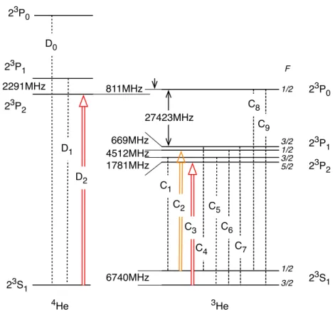
2 Amsterdam Experimental Setup 39 2.1 Helium atomic structure . . . 39
2.2 A Bose-Fermi mixture of metastable atoms . . . 40
2.3 Experimental sequence . . . 42
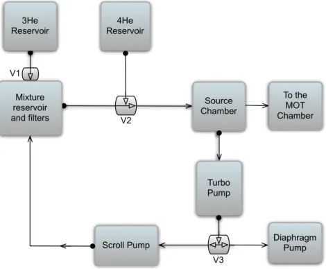
2.3.1 Source and recycling system . . . 43
2.3.2 Laser cooling transitions and laser system . . . 45
2.3.3 Atomic beam collimation . . . 47
2.3.4 The Zeeman slower . . . 48
2.3.5 The two species magneto-optical trap . . . 48
2.3.6 The Magnetic Trap . . . 50
2.3.7 Detection . . . 54
2.4 Conclusion . . . 56
3 Amsterdam-Palaiseau Experimental Results 57 3.1 Acquired Data . . . 58 3.1.1 Data analysis . . . 60 3.2 Experimental results . . . 65 3.2.1 Bosons-Fermions comparison . . . 65 3.2.2 Other temperatures . . . 68 3.2.3 Comments . . . 70 3.3 Defocusing experiment . . . 71 3.3.1 Experimental setup . . . 72 3.3.2 Experimental results . . . 73 3.3.3 Theory . . . 74 3.3.4 Dipolar force . . . 75
3.3.5 Calculation of the demagnification factor . . . 77
3.3.6 Results . . . 77
3.4 Conclusion . . . 78
II Correlated Atom Pairs 81 4 First Generation Experiment 83 4.1 Correlated pairs of photons . . . 84
4.1.1 Burnham and Weinberg (1970) . . . 84
4.1.2 Theory of the non-degenerate parametric amplifier . . . 85
4.1.3 Experiments with correlated photon pairs . . . 88
4.2 Correlated pairs of atoms . . . 90
4.3 Analogy with the parametric amplifier . . . 92
4.4 A more refined theory . . . 94
4.4.1 Analytical approach . . . 94
4.4.2 Numerical approach . . . 96
4.5 Experimental setup . . . 97
4.5.1 Production of two colliding condensates . . . 97
4.6 Experimental results . . . 100
4.6.1 Observation of the collision sphere . . . 100
4.6.2 Sphere thickness . . . 102
4.6.3 Back to back correlation . . . 104
4.6.4 Collinear correlation . . . 106
4.6.5 Mode occupancy . . . 109
4.6.6 Influence of the gain of the detector . . . 109
4.7 Comparison with theory . . . 110
4.7.1 Analytical calculation . . . 110
4.7.2 Positive-P calculation . . . 113
CONTENTS 3
5 Second Generation Experiment 119
5.1 Motivations for an upgraded experiment . . . 119
5.1.1 Sphere thickness and density . . . 119
5.1.2 Relative number squeezing . . . 120
5.2 New collision geometry . . . 123
5.2.1 Number of scattered atoms . . . 124
5.3 Experimental setup . . . 128
5.3.1 Theory of the Bragg transitions . . . 131
5.3.2 Spontaneous emission . . . 136
5.4 Preliminary results . . . 140
5.5 Conclusion . . . 142
Conclusion and outlooks 145 A The detector 149 A.1 The micro-channel plate . . . 149
A.2 The delay-line anode . . . 151
A.2.1 Working principle . . . 151
A.2.2 Electronic chain . . . 153
A.2.3 Determination of the position of the atoms in 3D . . . 154
A.3 Detector characteristics . . . 155
A.3.1 Pulse-height distribution . . . 155
A.3.2 Flux saturation . . . 156
A.3.3 Background noise . . . 158
A.3.4 Detection homogeneity . . . 159
A.3.5 Detection efficiency . . . 159
A.3.6 Detector resolution . . . 163
A.4 Influence of the resolution on the correlation function . . . 164
B Publications 167
Introduction
Optical interferometry was at the heart of the scientific revolution which lead to the new era of the twentieth century. Probably the most renowed example is the Michelson interferometer that was used to show that there is no detectable motion relative to “ether”, a key point in support of special relativity [1], [2]. In the same way Young’s interference experiments played a central role in the early discussion of the dual nature of light. At the end of the nineteenth century Young’s double slit interferometer could be completely described according to the classical theory of electromagnetism based on Maxwell’s equations and the wave nature of light seemed to be affirmed [3]. However, the situation changed radically in 1901 when M. Planck explained the ultraviolet catas-trophe problem by assuming that black-body radiation is emitted in discrete energy packets called quanta [4]. The first serious attempt to demonstrate the quantum nature of light was performed by G. I. Taylor in 1909. He set up a Young’s slit experiment and he reduced the intensity of the incident light beam to such an extent that there would be one photon incident on the slits at a time [5]. However, he didn’t see any difference between the interference pattern registered at low and high intensity. In fact the classical explanation based in the interference of electric field amplitudes and the quantum explanation based on the interference of probability amplitudes both explain this phenomenon. In order to see a difference between classical and quantum theory one should consider higher order interference experiments, such as intensity interference.
The pioneering experiment in intensity interferometry was performed by R. Hanbury Brown and R. Q. Twiss in 1956 [6]. This experiment studied the correlations between photons arriving at two different detectors. Hanbury Brown and Twiss showed an en-hancement of the probability for two photons, coming from a thermal light source, to arrive together on the two detectors, a phenomenon called photon bunching. Their experiment provoked a storm of controversy in the contemporary scientific community and the quantum explanation of the bunching effect was accepted only after the pub-lication of a fundamental paper by E. M. Purcell [7]. Although their results may be derived from both classical and quantum theory, the Hanbury Brown Twiss experiment marked the birth of the modern quantum optics, since the quantum theory makes addi-tional unique predictions. This was pointed out by R. Glauber in 1963 [8]. His work on quantum formulation of optical coherence theory was awarded in 2005 with the Nobel Prize [9]. One such prediction is photon antibunching, that was first observed by Kim-ble et al. [10] on photons spontaneously emitted by single atoms. At the same time,
the advent of laser sources gave access to other interesting quantum states of light, such as entangled states. The extraordinary character of entanglement, that has no classical counterpart, was at the center of debates since the early years of the quantum era [11], [12], [13], [14]. Realization of entangled states paved the way to new developments in quantum information and, in particular in quantum teleportation. These topics are nowadays still an open frontier of quantum physics. Other quantum effects such as amplitude and frequency squeezing were observed in four wave mixing and paramet-ric down conversion occurring in non-linear crystals and offered new possibilities for precision measurements and interferometry [15].
In parallel with the explosion of quantum optics, the recent progress in the manip-ulation of atomic states [16], [17], [18], [19] has led to several proposal for generating atomic states with properties similar to the ones of the nonclassical states of light. Photons and atoms are complementary under several points of view and experiments that are possible with atoms could not be possible with photons and vice-versa. For example, photons are well suited for transmission over long distances, but are difficult to store at a fixed location, while the reverse is true for atoms. In order to take advan-tage of the good properties of each system, there are several proposition of quantum atom optics experiments, involving single atoms, atomic ensembles or atom-photon pairs. Furthermore, a point of great interest for the development of quantum atom optics relies on a sharp distinction between photons and atoms: atoms can obey both quantum statistics, i.e. there are bosonic and fermionic atoms. This opens interesting perspectives for the realization of tests of fundamental principles of quantum mechanics with fermions and for a comparison of quantum effects for bosons and fermions, as in the case of the experiment described in the first part of this thesis.
Historically, the first candidates for quantum atom optics have been trapped ions. Since the early 1990s it has been possible to cool and trap single ions for a very long time (several days) and to perform quantum logic operations on them [20], [21]. An enormous amount of progress in this field has been made in the past twenty years and trapped ions are at the moment a leading candidate for quantum information and computing [22]. On the other hand, the achievement of Bose-Einstein condensation [23], [24], [25], made available to quantum atom optics the material analogue of laser. This analogy has been firmly established experimentally with the demonstration of spatial and temporal coherence of Bose-Einstein condensates [26], [27], which therefore deserve the name of matter waves. Not surprisingly as condensates became readily available in laboratories across the world, quantum atom optics saw the same kind of explosion as quantum optics after the developement of laser. The realization of atom lasers [28], atom mirrors and beam splitters [29] and atom interferometers [30], constitute a good example of the analogy between light and matter waves. Furthermore, the achievement of degenerate Fermi gases of neutral atoms [31], [32], [33] is particularly important for the reasons pointed out above.
Another significant step in the analogy between quantum optics and quantum atom optics has been made with the observation of four-wave mixing of matter waves [34], [35], [36]. In addition the generation of correlated atom pairs in the dissociation of cold
7 molecules [37] and in the collision of Bose-Einstein condensates [38] was demonstrated. The latter of these experiments has been performed in our group and is described in the second part of this thesis.
The simplest atomic system that has a bosonic and a fermionic isotope is Helium. Due to the fact that the ground state of Helium has no magnetic moment and that the only transition available for optical cooling is in the UV part of the spectrum, Bose-Einstein condensation is hard to achieve in the ground state. However, the triplet metastable state, that has a life time of the order of 7000 s, can be magnetically trapped and has atomic transitions suitable for laser cooling. Metastable Helium has been Bose-Einstein condensed for the first time in the Atom Optics group of the Labora-toire Charles Fabry de l’Institut d’Optique [39]. The metastable Helium experiment is supervised by C. Westbrook, D. Boiron and A. Aspect. It constitutes an original setup for the study of atom optics especially for its detector. In fact the large internal energy of the metastable state makes possible to perform single atom detection, resolved in space and time. This detector allows us to reproduce quantum optics experiments that involve single photon counting.
When I joined the He* team in october 2005 to start my PhD thesis, the detector had been installed one year earlier and the Hanbury Brown Twiss effect on a cold cloud of bosons above and below the condensation threshold had been observed [40]. Almost at the same time the group of W. Vassen at the Laser Centre of the Vrije Universiteit succeeded in the production of degenerate Fermi gas of metastable Helium [41]. There-fore in July 2006 we brought the detector to Amsterdam for two months and, after having inserted it in the existent experimental apparatus, we measured the Hanbury Brown Twiss effect on a cold cloud of fermions [42]. Furthermore we could compare the correlation functions for clouds of bosons and fermions at the same temperature, created in the same experimental apparatus, highlighting the different statistics obeyed by the two systems. The preparation of the collaboration was committed to Martijn Schellekens, another PhD student, and me. We spent the ten months before leaving for Amsterdam in studying in detail the characteristics of the detector.
At the same time Aur´elien Perrin as PhD student and Hong Chang as a post-doc performed an experiment aimed at the creation of correlated pairs of atoms by the collision of two Bose-Einstein condensates. The correlation between pairs of atoms was demonstrated and the correlation function was studied in detail in three dimensions, thanks to the use of our detector [38]. This experiment constitutes the atomic analogue of the generation of correlated photon pairs in parametric down conversion or four-wave mixing [43].
In order to perform a more detailed study on correlated pairs we decided to repeat the experiment in an improved version. Unfortunately, the moving from Orsay to Palaiseau in June 2007 imposed a break in our scientific activity. For the dismounting and the reconstruction of the setup in the new building I was helped by Jean-Christophe Jaskula and Vanessa Leung that recently have joined our team as a PhD student and a post-doc respectively. After producing a Bose-Einstein condensate in February 2008, the experimental setup was again fully functional. In 2008, another post-doc, Guthrie
Partridge, and a PhD student, Marie Bonneau, joined our group. Together we finally succeeded in fixing the experimental problems and we started data acquisition. The data analysis is cumbersome and has to be done with great care. Some preliminary results are available at this moment and are reported at the end of this thesis.
Outline of this thesis
This thesis is devoted to the description of the two experiments performed during my PhD, the observation of fermionic antibunching and the creation of correlated atom pairs by condensate collision.
This thesis is divided in two parts. The first part is devoted to the fermionic Hanbury Brown Twiss effect and is divided in three chapters. In the first chapter an historical overview of the Hanbury Brown Twiss effect is given, together with an explanation of the Hanbury Brown Twiss effect in terms of quantum theory. A more refined theory is derived in order to describe the correlation function for a gas of fermions above and below degeneracy in an harmonic trap. In the second chapter we describe the experimental setup used during the collaboration with the group of W. Vassen. A comparison with our experimental setup is drawn and a special attention is payed to the upgrades that would be necessary on our experiment in order to cool the fermionic Helium isotope. In the third chapter we show the experimental results obtained during the collaboration.
The second part of this thesis is devoted to the correlated pairs experiment. It is divided in two chapters. In the first one we describe the quantum optics analogue of our experiment and some fundamental experiments in quantum optics and quantum atom optics that are useful to set the context of our measurements. We then describe the experimental setup and the obtained results. In the second chapter we explain in detail the motivation for the upgraded version of the experiment and we thoroughly compare the two experiments. The new experimental setup is then described and some preliminary results are showed.
Part I
The Hanbury Brown Twiss effect
for fermions
Chapter 1
The Hanbury Brown Twiss effect
This chapter is devoted to the Hanbury Brown Twiss effect. We will first give an historical overview, highlighting the reasons why the experiment carried out by the two astronomers in the 1950’s, was seminal in the development of the modern quantum optics. In the second part of the chapter we will show the substantial difference in the Hanbury Brown Twiss effect for bosons and fermions. Since the Hanbury Brown Twiss effect for bosons has been studied in several other thesis of the group ([44], [45]), we will concentrate on the experiments done on fermionic samples, as electrons in semiconductors, electrons in vacuum, neutrons and neutral atoms. In the third part we will present the theory that describes the experiment done in a collaboration between our group and the group of W.Vassen in Amsterdam, where we observed the Hanbury Brown Twiss effect on a cold cloud of 3He (fermionic Helium isotope) and of 4He (bosonic Helium isotope) [42]. We will concentrate on the theoretical formula of the 2-body correlation function for a fermionic sample of ultracold atoms released from a harmonic trap, indicating in particular the influence of the finite detector resolution on the correlation length and on the antibunching height. The experimental apparatus and the experimental results will be described in details in chapters 2 and 3.
1.1
Brief history of the Hanbury Brown Twiss effect
The radar technology developed during the Second World War opened the field of radio astronomy and led very quickly to the discovery of bright radio sources in the sky. Since their size was unknown, astronomers raised the problem of how to measure it. Since then, the angular size of a star was measured with Michelson interferometer, that is based on a Young’s double slit like interferometer. The Michelson stellar interferometer is sketched in figure 1.1.
In Michelson interferometry one compares the amplitudes of the light landing at two separated points. The distance between the two points is equal to the distance between the two slits drawn in figure 1.1. If the separation is not too large, the two signals can be superposed using a lens. The produced diffraction pattern varies as a function of the separation of the slits. At a given point P on the screen the amplitude
Star
Atmosphere
Young's double slit Screen P Lens x y t a d
Figure 1.1: Michelson stellar interferometer. The outer mirrors send the light through a Young’s double slit interferometer. The distance between the slits and the screen is a and the distance between the two slits is called d. The diffraction pattern is detected on the screen below the double slit.
of the light will be given by the sum of the amplitudes transmitted by the two slits, A1(t) and A2(t + τ ). The time τ represents the time difference for the light to reach P from each slit. The intensity observed on the screen at the point P will then be given by
IP = !|A1+ A2|2"t= I1+ I2+ 2Re(Γ12(τ )) (1.1) Γ12(τ ) = !A1(t)∗A2(t + τ )"t
The latter term takes account of the observed interference pattern. In case of an extended source the interference pattern varies over a typical distance, called coherence length of the source, of the order of λ/θ, where θ is the angular size of the source. A more detailed treatment of the Michelson interferometer can be found in [3] and [46].
It is clear that, in order to perform a measurement with an amplitude interfer-ometer it is crucial to precisely measure the phase difference between A1 and A2. If atmospheric perturbations or mechanical instabilities in the telescope make the path difference change during the acquisition time, interference fringes can be blurred out. In addition, the resolution in amplitude interferometry at a given wavelength is given by the distance over which one is able to compare the amplitudes and their phases. Therefore, if the star has a small angular size, it can be necessary to separate the mir-rors (i.e. the two slits) by very large distances. In this case it might be impossible to recombine the signals on the same point of the screen and the use of coherent inde-pendent oscillators might be necessary. Since this technology was not available in the early 1950’s, R. Hanbury Brown and R. Twiss decided to perform the measurement in an alternative way, by doing intensity interferometry [47]. A schematic view of the intensity interferometer is drawn in figure 1.2.
Brief history of the Hanbury Brown Twiss effect 13
S
1S
2I
1I
2d
D
1D
2Figure 1.2: Scheme of the intensity interferometer. The light coming from a star is detected on two detectors separated by a distance d. The correlation between the detected intensities I1 and I2 is then
measured.
The radiation emitted by the star is collected on two independent detectors. The intensities measured at the two detectors are: I1 = A∗1A1 and I2 = A∗2A2. Then one measures the correlations between the two detected intensities as a function of the dis-tance between the detectors, i.e., the quantity !I1I2" where ! " indicates the average over random phases. Since the correlated signal varies as a function of the detector separation d on a distance of the order of the correlation length, an intensity interfero-metric measurement gives the angular size θ of the star. A more detailed explanation of the Hanbury Brown Twiss effect in terms of classical electromagnetic waves can be found in [48]. A familiar example of the Hanbury Brown Twiss observation is the speckle pattern. When a non-pointlike incoherent light source illuminates a screen, a large number of patches appears on the screen and the image is not homogeneous as one would naively expect. This random intensity pattern is produced by the inter-ference between the optical waves. The characteristic size of the speckle grain on the plane of the screen is of the order of the spatial coherence of the beam and it is called correlation length. The characteristic time over which this pattern changes is called coherence time. We will come back on this three-dimensional aspect of the correlation in the following sections.
The radio sources that the Hanbury Brown Twiss interferometer was intended to measure, turned out to be resolvable within few kilometers, therefore the measurement could have been performed with an amplitude interferometer as well. R. Hanbury Brown was so disappointed that he described intensity interferometry as “a steam roller to crack a nut” [49]. However, the importance of the intensity interferometer was not only related to astronomical measurements. In fact, while it was accepted and demonstrated theoretically and experimentally that intensity interferometry worked for radio waves, it was not clear that the effect should also work for light. The fact that
light was made by photons was still debated at that time and Hanbury Brown and Twiss decided to test their intensity interferometer in a table-top experiment in which they measured the intensity correlation of the light emitted by a mercury lamp [6]. The experimental setup and the obtained results are reported in figure 1.3.
2.0 1.5 N o rma lise d co rre la ti o n g (2 )(d ) Detector Separation d/mm 0 5 10 Theory
Figure 1.3: On the left: Experimental setup used by Hanbury Brown Twiss for the table-top experiment that proves the particle nature of light. The figure has been taken from [6]. On the right: Experimental results. The intensity correlation for coincident detectors results to be twice bigger than the value obtained when the detectors are far apart. In this case we find the value that we would have obtained for statistically independent particles. This figure has been taken from [50] and has been adapted from the data obtained in [6].
The light of the mercury lamp was split into two beams on a half silvered mirror and the intensity of each beam was measured on a photomultiplier. One of the photodetector could be spatially moved, so that the angular separation of the two detectors as seen from the source could be changed. Therefore it was possible to measure the intensity correlation as a function of the detector separation like in the stellar interferometer. From the point of view of a stream of photons, measuring intensity correlation amounts to measure the joint detection probability of two independently emitted photons on two independent detectors. The measurement showed that the detection probability, when the detectors are close together, is twice larger than the value obtained when they are far apart. When the detectors are far apart one finds the value that one would have obtained for statistically independent particles. The “photon bunching” was therefore demonstrated and quantum optics was born. In a second table-top experiment Hanbury Brown, Twiss and Little [50] measured the time correlation between photons emitted from the same source. The experimental setup was similar to the one of fig. 1.3, but a time-delay could be inserted before one detector in order to measure the correlation as a function of time. The obtained results showed again a photon bunching. The scientific community was sceptical about their results and several experiments were done to disprove them. At the end Hanbury Brown and Twiss won the day, helped by an important paper of E. M. Purcell [7], that explained the effect in terms of quantum mechanics. In addition to a mathematical explanation, Purcell gave a strong example to prove that the observed effect was a pure quantum mechanical effect:
“Were we to carry out a similar experiment with a beam of electrons, we should, of
enhance-To bunch or not to bunch? 15
ment; the accidentally overlapping wave trains are precisely the configurations excluded by the Pauli principle. Nor would we be entitled in that case to treat the wave function as classical field.”[7]
If for photons, that are bosons, bunching can be explained with a semi-classical theory, it is impossible to explain antibunching for fermions without the aid of quantum mechanics. Fermions are, in this sense, ”more quantum” than bosons. In the next section we will explain the Hanbury Brown Twiss effect for bosons and fermions with a simple calculation of quantum mechanics.
1.2
To bunch or not to bunch?
As we said in the previous section, in order to understand the Hanbury Brown and Twiss effect we have to answer the questions:
“How large is the joint detection probability of two particles on two detectors?” and:
“Does it depend on the statistics of the considered particle?”
To find the answer one has to calculate the two-body correlation function g(2)(d), where d, as in the previous section, is the distance between the two detectors.
Consider two particles emitted by two source points S1 and S2 and two detectors D1 and D2 (see figure 1.4). If we record a click on D1 and one on D2, we could have
S
1S
2D
1D
2S
1S
2D
1D
2Figure 1.4: Two particles emitted by the two source points S1and S2 are detected at D1 and D2. The
two particles can follow two paths that are sketched in this figure. The interference between the two paths leads to the Hanbury Brown Twiss effect.
detected a particle emitted from S1 on D1 and a particle from S2 on D2 (configuration sketched in figure 1.4 left), or a particle emitted from S1 on D2 and vice versa (see figure 1.4 right). The source state vector, for two identical particles, can be written as:
|ψ(S1, S2)" = √1
2(|S1S2" ±| S2S1") (1.2) If the two particles are identical bosons the state vector has to be symmetric for particle exchange (+ sign in the equation above), if they are identical fermions it has to be antisymmetric (− sign). When the two particles are detected, the source state vector,
after temporal evolution, is projected on the two detector state |D1D2". The joint detection probability is then given by:
P (D1, D2) = |!D1D2|ψ(S1, S2)"|2 = 1 2(|!D1D2|S1S2"| 2+ |!D 1D2|S2S1"|2± ± 2 Re !D1D2|S1S2"!D1D2|S2S1") (1.3) where the + sign holds for bosons and the - sign holds for fermions.
If the two particles are statistically independent, then: PIndep(D1, D2) =
1
2(|!D1D2|S1S2"|
2+ |!D
1D2|S2S1"|2) (1.4) irrespective of the distance between the two detectors. On the other hand, for a sample of identical particles, the correlation function (i.e. P (D1, D2)) will depend on the detector separation and its value, for a small distance between the detectors, will depend on the nature of the particle. For null detector separation, we will have !D1D2|S2S1" = !D1D2|S1S2" and the joint detection probability will be:
PBose(D1≡ D2) = (|!D1D2|S1S2"|2+ |!D1D2|S2S1"|2) = 2 × PIndep (1.5) if the two particles are identical bosons, and
PF ermi(D1≡ D2) = 0 (1.6)
if the two particles are identical fermions. As we pointed out in the previous section, bosons arrive bunched on the detector and the probability of finding two bosons is twice the probability for independent particles. On the other hand, fermions tend to “antibunch”, because for the Pauli exclusion principle they cannot occupy the same quantum state.
In the case of an extended source, as we increase the detector separation, the corre-lation function will tend in both cases to the value obtained for independent particles with a shape that is given by the interference term in equation 1.3. The typical dis-tance over which the correlation function goes to the independent particles value is called correlation length. In section 1.4.1 we will derive the formula of the correlation function of a cold fermionic cloud released from a harmonic trap. Figure 1.5 sketches the shape of the correlation function for a sample of identical bosons, fermions and independent particles.
In the treatment above we assumed an ideal detector, i.e., with arbitrarily good resolution. The effect of the finite detector resolution and efficiency will be treated at the end of the chapter (section 1.4.5). For the moment we just note that, if the correlation length is too small to be resolved, the correlation function will be broader and the contrast will be smaller than 1. In other words, the finite resolution makes the measured correlation length larger, but doesn’t change the number of correlated pairs, i.e. the bunching (antibunching) area.
Experiments with fermions 17
Lc
0
1
2
g
(2)bosons
fermions
Figure 1.5: Correlation function for a sample of statistical independent particles (dashed line), a sample of identical non-interacting bosons and identical fermions. The correlation function has been normalized with respect to the value obtained for statistical independent particles.
1.3
Experiments with fermions
The Hanbury Brown Twiss effect for fermions has been observed with electrons, neu-trons and neutral atoms. The peculiarity of the last system is that the same atomic species can have bosonic and fermionic isotopes and a direct comparison of the two correlation functions can be made. It is the case of the experiment done in the col-laboration between our group and the Amsterdam group with 3He and 4He [42]. We will treat the theory underlying the measurement at the end of this chapter, while the experimental apparatus and experimental results will be described in chapter 2 and 3 respectively.
In this section we will describe the other experiments where the Hanbury Brown Twiss effect was measured on a sample of fermions. An overview of the experiments done with bosons can be found in [44].
Before starting this brief review, we want to clarify the three dimensional character of the two-body correlation function that we noted in section 1.1. We can identify two kinds of experiments, the ones where the detectors receive a continuous flux of particles and the ones where the entire sample is probed with a snap shot image. If the Hanbury Brown Twiss measurement is done over a continuous flux of particles, one has access to g(2)(∆x, ∆y, ∆t), i.e., to the measurement of the spatial correlation length on the plane xy, orthogonal to the particle propagation direction, and to the time correlation length along the direction of propagation. This is the case of the speckle measurement that we described in section 1.1, as well as of the Hanbury Brown Twiss table-top experiment and, in the following overview, of the experiments done with electrons [51],[52],[53] and neutrons [54]. On the other hand, if the experiment is carried out on a pulsed beam of particles and the detection time is small with respect to the dynamics of the system
(the detection is a snap shot), then the three directions of space are equivalent and one will have access to g(2)(∆x, ∆y, ∆z). This is the case of the experiments done with cold atoms [55], [42], where either absorption imaging or a micro-channel plate is used to perform the detection. In the case of the micro-channel plate detection, what we said is valid only under the condition that the cloud doesn’t expand while passing through the plate, as we will see in section 1.4.4.
1.3.1 Experiments with charged fermions
Electrons in mesoscopic conductors
The first experiments that observed the antibunching were carried out with electrons in mesoscopic conductors [51], [52], [56], more than 40 years after the first observation on photons. In fact, the statistical effects measured in the correlation function depend on the occupation of the available states. Reaching the degeneracy regime, i.e. unit occupation of all the states below the Fermi energy, was possible in 1999 for electrons in mesoscopic conductors at very low temperature. In this year, Henny et al. [52] and Oliver et al. [51] performed two very similar experiments. The scheme of the experimental setup is shown in figure 1.6.
V I r 3 I beam splitter B 2 1 t=1/2 p I t IN T R f a-). a- r-m r-es g) ly y, o Bosons Fermions correlations anti-correlations IN R T
Figure 1.6: On the left, simplified scheme of the setup used by Henny et al. and Oliver et al. to measure the Hanbury Brown Twiss effect on a beam of electrons in a mesoscopic conductor. The figure has been taken from [57]. On the right, an illustration of the different statistics describing bosons and fermions and the expected correlations (anticorrelations) at the output of the beam splitter.
The current injected in the mesoscopic conductor from contact 1 travels in the conductor until reaching a 50% beam splitter. The transmitted beam is then collected on the contact 2 and the reflected beam is collected on contact 3 and the correlation between the transmitted and reflected current is measured. The variable transmission of the barrier between contacts 1 and 3 allows to vary the coherence of the electron currents. To understand this let’s imagine a system of electrons where all the states are occupied by one fermion (i.e. at zero temperature). The system will be fully anticorrelated. Varying the transmission through the first barrier, amounts to empty some of the states, with a distribution that is random in time. Therefore, if the sample
Experiments with fermions 19 was degenerate for a 100% transmission efficiency (i.e. all the states with a temperature smaller than the Fermi temperature were occupied), it is no longer the case when the efficiency is reduced. In other words one can artificially increase the temperature of the sample thereby decreasing its time correlation length.
Both groups were able to demonstrate that, varying the transmission of the first barrier, it is possible to pass from a regime where the currents measured at contacts 2 and 3 are fully anticorrelated to a regime where the statistic of the beam incident on the beam splitter is Poissonian and the anticorrelation vanishes.
Beam of free electrons
A few years later (2002) the Hanbury Brown Twiss effect was observed on a beam of electrons in vacuum by Kiesel and collaborators [53], [58]. Due to the difficulty to achieve the degeneracy, observing anticorrelations in vacuum was more difficult than in mesoscopic conductors. In order to perform the experiment, Kiesel et al. used a very bright source, where the states occupation was close to one electron per interval of coherence time. Their experiment mimics the stellar interferometer (see figure 1.7, left): an electron field emitter illuminates two detectors and coincidences in the arrival time of the electrons at the two detectors are measured.
Figure 1.7: On the left, simplified scheme of the setup used by Kiesel et al. to measure the Hanbury Brown Twiss effect on a beam of electrons in vacuum. The figure has been adapted from [53]. On the right, time coincidences for incoherent illumination (dashed lines) compared to coherent illumination (full line). A reduction of the number of coincidences is shown.
Before arriving on the detectors, the electron beam passes through a lens. Changing the magnification amounts to vary the effective lateral distance between the detectors and their illumination changes from incoherent to coherent. The authors repeated the correlation measurement for different magnification factors, showing a reduction of the number of coincidences for a coherent illumination with respect to an incoherent
illumination (see figure 1.7, right). As expected from theory, the antibunching height was only of 10−3, but it was enough to demonstrate the existence of anticorrelation.
1.3.2 Experiments with neutral fermions
Since electrons are affected by Coulomb repulsion, one can argue that anticorrelations observed in charged system are due to electrostatic repulsion. Actually the Coulomb force is small and cannot explain the observed antibunching, but scientists found inter-esting to repeat the Hanbury Brown Twiss experiment with samples of non-interacting fermions, such as neutrons or cold atoms. In the following sections we will describe those experiments.
Beam of free neutrons
In the “News and Views” [58] associated to the paper of Kiesel et al., J. C. H. Spence affirms that reaching the degeneracy in a beam of neutrons would have been even more difficult than for electrons, “making the observation of neutron anti-bunching a
hope-less endeavour”. Neverthehope-less, the observation of neutron antibunching by means of
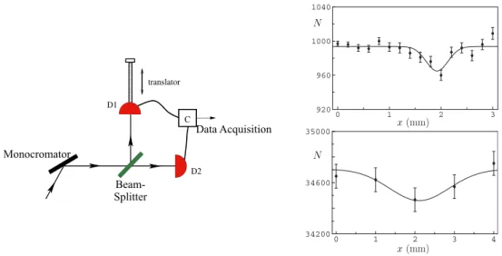
coincidence measurements on a neutron beam was realized in 2006, thanks to technol-ogy development, that made precise instrumentation and a precise knowledge of the statistical properties of the source available. In an experiment carried out in Greno-ble, Iannuzzi et al. [54] measured the Hanbury Brown Twiss effect on such a beam, observing the antibunching and measuring the correlation time of the source. The experimental setup is sketched in figure 1.8 on the left.
A monocromatic beam of thermal neutrons is split in two by a beam splitter. The intensity of each beam is then measured on two detectors and the intensity correlation is measured as a function of the relative distance of the detectors from the source. In order to vary the detector separation, one of the detectors can be moved, parallel to the beam propagation. This amounts to introduce a delay between the detection of the two beams and therefore it gives access to g(2)(0, 0, ∆t). Care was taken in the choice of the beam splitter and the detectors in order to reduce any additional spread of the signal. The authors repeated the experiment with two kinds of detector, a gas detector and a scintillator. The major difference between the two resides in the time resolution, that is worse for the gas detector than for the scintillator, and in the translation step, that is bigger for the gas detector than for the scintillator. The first quantity has to be compared to the coherence time and will determine the antibunching height. The number of coincidences as a function of the detector separation is reported in figure 1.8 on the right. The top panel reports the measurements obtained with the scintillators and the bottom panel with the gas detector. With an accurate fit the authors can determine the correlation time and the antibunching height, that are consistent with theory.
Experiments with fermions!!!!!!! 21 x(mm) x(mm) N N 0 1 2 3 920 960 1000 1040 0 1 2 3 4 34200 34600 35000 D1 D2 translator C to DAE M S Monocromator Beam-Splitter Data Acquisition
Figure 1.8: On the left, scheme of the setup used by Iannuzzi et al. to measure the Hanbury Brown Twiss effect on a thermal beam of neutrons. The figure has been adapted from [54]. On the right, number of coincidences N as a function of the detector separation. In the top panel the measurements done with the scintillator detector are reported, in the bottom panel the measurements done with the gas detector. The detector separation can be converted in time difference with the formula t = (x−x0)/v
where x0 is the dip center (that depends on detector calibration) and v is the neutron speed (about
630 m/s).
Cold atoms in an optical lattice
The group of I. Bloch performed in Mainz in 2006 a measurement of the Hanbury Brown Twiss effect in a degenerate Fermi gas of 40K released from an optical lattice [55]. This experiment is the fermionic counterpart of an experiment done by the same group one year earlier on the Mott insulator phase of a rubidium Bose gas [59]. In the fermionic experiment, the atoms are first cooled below the Fermi temperature and then loaded in a three-dimensional optical lattice. The lattice is suddenly switched off and, after a time-of-flight of 10 ms, the atoms are imaged on a CCD camera via standard absorption imaging along the vertical axis. The position of the atoms after the time-of-flight corresponds to their momentum distribution in the trap.
In the lattice, the atoms occupy Bloch states in the lowest energy band. Each Bloch state is characterised by a crystal momentum ¯hq, where q is the crystal wave vector, defined in the first Brillouin zone of the reciprocal lattice. Due to the periodicity of the Brillouin zone, each Bloch state is a superposition of states with momentum ¯hq + 2n¯hk, with n an integer number and k the wave vector of the laser used to create the lattice. When a particle with quasi-momentum ¯hq is released from the lattice, it has equal probability to be detected at any of the positions xn= (¯hq + 2n¯hk)t/m, where t is the duration of the time-of-flight and m is the mass of the particle. Conversely, if a particle has been detected at the position xn, it has to come from a state of the crystal with quasi-momentum ¯hq. Now, since we are dealing with identical fermions, the occupation
of a single Bloch state by two particles is not allowed by the Pauli principle. Therefore it will be impossible to detect a particle in the position xnand a particle in the position xn′. Since the positions xn are equally spaced by l = 2¯hkt/m, the spatial correlation
will vanish for any distance |xn− xn′| integer multiple of l.
Figure 1.9: On the left: a. Single shot absorption image of the fermionic cloud released from an optical lattice. The inset shows the occupation of the Brillouin zones, demonstrating that only the lowest is occupied. b. Horizontal cut of image a. No spatial structure is present. On the right: c. Correlation measured on 158 shots like that of figure a. A rectangular periodic array of black dots is visible, the dots are circled by a solid black line. The horizontal profile through the centre of the correlation shows that the the dots correspond to dips, spaced by l. The figure has been taken from [55].
In figure 1.9 we show the experimental results. On the left the image recorded after the time-of-flight is reported. No periodic structure is present (as shown by the one-dimensional cut through the image centre, figure 1.9 bottom left). On the right is shown the correlation function obtained from the analysis of 158 images. A rectangular periodic array of peaks is visible. A horizontal profile through the centre of the image (bottom right) shows that the amplitude of the peaks is negative and that they are spaced by a multiple of l, as expected as a signature of the Hanbury Brown Twiss effect.
It is interesting to make a few comments on the imaging technique that has been used in this experiment. In general absorption imaging allows one to measure the column density of the atomic cloud, but it is not a single particle detection. The measurement of second order correlations is then tricky and, in 2004, Altman et al. [60] proposed for the first time to use this technique to measure spatial correlations in fermionic superfluids and clouds released from an optical lattice. They proposed to measure atom shot noise in the time-of-flight images. This is possible only if atomic shot noise dominates over the shot noise of the absorbed beam and on the technical noise. This requirements are hard to achieve with current CCD cameras.
In this perspective the enormous advantage of using metastable helium atoms is that one can easily perform single atom detection in three dimensions. Measuring
Experiments with fermions 23 second order correlation functions is much easier with a single atom detector, than with absorption imaging. With this kind of detector our group measured, in 2005, the correlation function of a thermal cloud of bosons and of a Bose-Einstein condensate [40]. In 2006 we were able to measure the same quantity for a cloud of bosons and fermions [42]. As we already pointed out this will be the subject of chapters 2 and 3. Here we only briefly outline it in order to complete our review of the measurements of the HBT effect on fermions.
Amsterdam-Palaiseau experiment
An artistic view of the setup is reported in figure 1.10. A cold cloud of metastable3He (fermions) or4He (bosons) atoms can be prepared with standard cooling techniques in a magnetic, cigar shaped, trap (see chapter 2). When the desired temperature is reached the trap is suddenly switched off and the atoms fall, under the effect of gravity, on the detector, situated 63 cm below the trap centre. The trap frequencies are ωx/2π = 54 Hz and ωyz/2π = 506 Hz for 3He and ωx/2π = 47 Hz and ωyz/2π = 440 Hz for 4He. We acquired data with samples of 3He and 4He at a temperature of 0.5 µK in order to be able to make a comparison between the correlation function of bosons and fermions at the same temperature. We also acquired3He cold clouds at 1 µK and 1.5 µK to follow the change of the fermionic correlations as a function of the temperature.
Figure 1.10: Sketch of the experimental setup used in the Amsterdam-Palaiseau experiment. A meta-stable helium cloud is released at the switch-off of the magnetic trap. The atoms fall under the effect of gravity on a 3D single atom detector situated 63 cm below the trap.
The detector is a micro-channel plate with a delay-line anode (see appendix A for technical details), capable to record the position of the single atoms on the xy plane and their arrival time on the detector (i.e. the vertical position). The time-of-flight is very long (about 360 ms) and the position of the atoms measured on the detector reflects the momentum of the atoms in the trap. After the detection we can measure the two-body
correlation function of the atomic cloud by just measuring the probability of finding an atom at a certain distance from another one (all the details of the data analysis will be given in chapter 3). In the next section we will derive the theoretical formulation of the second order correlation function that we will compare with the obtained experimental results presented in chapter 3. The major result obtained in this collaboration is the
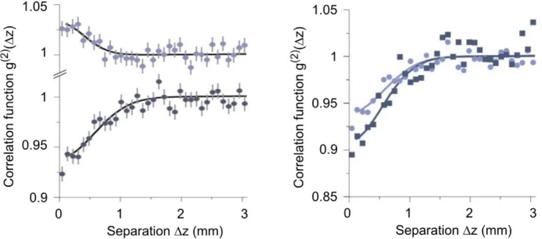
1 1.05 0.95 0.9 1 C o rre la ti o n f u n ct io n g (2 )(! z) 0 1 2 Separation !z (mm) 3 1 1.05 0.9 0.85 0.95 C o rre la ti o n f u n ct io n g (2 )(! z) 0 1 2 Separation !z (mm) 3
Figure 1.11: On the left: Two-body correlation function along the z direction for a cloud of4He (upper
graph) and a cloud of 3He (lower graph) at 0.5 µK. The different quantum behavior of bosons and fermions is clearly visible. The error bars correspond to the square root of the number of entries in each bin. On the right: Correlation function along the z axis measured on a fermionic cold cloud at 0.5 µK. The light blue curve is the same as the one shown on the left side of the figure. The dark blue is the correlation obtained when the effective size of the source is made smaller by the application of a blue detuned laser during the time-of-flight. The contrast of the correlation function is increased.
measurement of the two-body correlation function in three dimensions in space for a sample of fermions and a sample of bosons at the same temperature and in the same experimental apparatus. Our detector allows us to perform quantitative measurements of the correlation lengths. The two-body correlation function along the z (vertical) axis is shown in figure 1.11 (left). As expected we observe a bunching for bosons (upper graph) and an antibunching for fermions (lower graph). The correlation lengths resulted to be inversely proportional to the angular size of the source as seen from the detector. The comparison between correlation measured for bosons and fermions showed that the correlation lengths are different due to the different mass of the two isotopes. The contrast of the correlation function is limited by the detector resolution. We also measured the correlation length for fermions as a function of the temperature of the sample. The measured values are in good agreement with the theory developed in section 1.4.
In a second experiment we artificially changed the size of the source by shining a blue-detuned laser on the atomic cold cloud during the time-of-flight. The effective source is then smaller than the trapped source and the correlation length at the detector is larger. This way one can hope to increase the correlation length to a value larger
Theory for a ballistically expanding fermionic cloud 25 than the detector resolution and to see the correlation function going down to zero. The performances of our atomic lens were not that good but we could observe an increase in the contrast of the correlation function of a factor 1.4. In figure 1.11 (right) we report the measured correlation function along the z axis with (in blue) and without (in light blue) the application of the atomic lens. The difference is clearly visible. In section 3.3 we will discuss this experiment in detail.
1.4
Theory for a ballistically expanding fermionic cloud
In this section we will derive the theoretical expression of the two-body correlation function for a cloud of ultracold non-interacting fermions released from a harmonic trap.
In section 1.4.1 we will derive the expression of the correlation function for a non-interacting gas of fermions at thermal equilibrium in a trapping potential. Among the data acquired during our collaboration the 3He clouds at 0.5 µK were degenerate (T /TF ≈ 0.66), therefore we will derive the expression of the correlation function for a degenerate trapped cloud and we will compare it with the result found for a non-degenerate cloud.
In section 1.4.4 we will derive the expression of the correlation function after a ballistic expansion.
At the end of the chapter we will discuss the effect of the finite detector resolution and the finite detectivity on the correlation function (sec. 1.4.5).
1.4.1 Correlation function for a trapped cloud
Consider a cold cloud of identical (spin polarized) fermions confined in a trapping potential. The sample is at thermal equilibrium at the temperature T. The trapping potential is characterised by the parameters ǫj and φj, the energy and the wave function of the level j. In second field quantisation, the field operators are defined as:
ˆ Ψ†(r) =! j φ∗j(r)ˆa†j, Ψ(r) =ˆ ! j φj(r)ˆaj (1.7)
The operator ˆa†j (ˆaj) annihilates (creates) a particle in the state j and the field operator ˆΨ†( ˆΨ) annihilates (creates) a particle at the position r. Since we are dealing with fermions, the system follows the Fermi-Dirac distribution and !ˆa†jˆak" = δjk(1 + exp{β(ǫk−µ)})−1, where β = (kBT )−1, with kBthe Boltzmann constant. The quantity µ is the chemical potential and its value ensures that"
j!ˆa†jˆak" = N, the total number of particles in the system. In addition the field operators defined above will obey to the following commutation rules:
{ ˆΨ(r), ˆΨ†(r′)} = δ(r − r′) { ˆΨ(r), ˆΨ(r′)} = 0
If one neglects the shot noise term, the second order correlation function is given by:
G(2)(r, r′) = ! ˆΨ†(r) ˆΨ(r) ˆΨ†(r′) ˆΨ(r′)". (1.8) We shall define two other quantities that will be useful in the calculation of 1.8, the first order correlation function G(1)(r, r′) and the density of the sample ρ(r):
G(1)(r, r′) = ! ˆΨ†(r) ˆΨ(r′)" (1.9) ρ(r) = ! ˆΨ†(r) ˆΨ(r)" = G(1)(r, r) (1.10) If we go back to the beginning of this chapter, we see that equation 1.9 is the quantum formulation of equation 1.2 (the product of two amplitudes), while G(2) is the quantity measured in intensity interferometry (the product of two intensities). If we inject 1.7 in 1.8 we obtain:
G(2)(r, r′) = ! j,k,l,n
φ∗j(r)φk(r)φ∗l(r′)φn(r′)!ˆa†jˆakˆa†laˆn" (1.11)
The Wick’s theorem [61] allows to write:
!ˆa†jˆakaˆ†laˆn" = !ˆa†jaˆj"!ˆa†kˆak"(δjlδkn− δjnδkl) + !ˆa†jˆaj"δklδjn (1.12) that, injected into 1.11, using the definitions 1.9 and 1.10, leads to:
G(2)(r, r′) = ρ(r)ρ(r′) − |G(1)(r, r′)|2+ ρ(r)δ(r − r′). (1.13) The last term is called shot-noise term and will be neglected in the following because it is proportional to the number of atoms N while the other terms are proportional to N2. We can now calculate the normalized correlation function:
g(2)(r, r′) = G
(2)(r, r′) ρ(r)ρ(r′) = 1 −
|G(1)(r, r′)|2
ρ(r)ρ(r′) (1.14)
We can make some remarks about the expression of g(2) that we just found. For a bosonic sample far from the critical temperature the expression of g(2) is the same as for fermions, but with a + sign instead of a - sign in front of the last term. It is this sign that gives rise to bunching for bosons and antibunching for fermions. In fact, for r = r′, |G(1)(r, r)|2 = ρ(r)ρ(r) and then g(2)(r, r) = 2 for bosons and g(2)(r, r) = 0 for fermions. Moreover, if the cloud has a finite correlation length, G(1)(r, r′) → 0 when |r − r′| →∞ and g(2) tends to 1, the value obtained for two independent particles.
If the temperature is closed or below the transition temperature (the Fermi temper-ature for fermions, the critical tempertemper-ature for bosons), the equation 1.14 is still valid for fermions but not for bosons. In fact the population of the ground state is macro-scopic for bosons close to the condensation threshold and the second order correlation function becomes [62]: g(2)BEC(r, r′) = 1 +|G (1)(r, r′)|2 ρ(r)ρ(r′) − ρ0(r)ρ0(r′) ρ(r)ρ(r′) (1.15)
Theory for a ballistically expanding fermionic cloud 27 where ρ0(r) is the ground state density. Since for a Bose-Einstein condensate at T = 0 only the ground state is occupied, then |G(1)(r, r′)|2 = ρ(r)ρ(r′) = ρ0(r)ρ0(r′) and therefore g(2)BEC(r, r′) = 1.
For a degenerate gas of fermions this doesn’t occur and equation 1.14 is still valid. In the following section we will derive the expression of g(2)(r, r′) for a sample of fermions trapped in a harmonic trap, as in case of the Amsterdam-Palaiseau experiment, and we will study the behaviour of the correlation function close to the Fermi temperature.
1.4.2 Density and correlation function for a harmonic trap
Calling ωα the trap oscillation frequencies along the α direction, we can write the hamiltonian of the system as:
ˆ H = pˆ 2 2m+ 1 2m( ! α ω2αr2α) (1.16)
The eigenfunctions of the system, for the level j with energy ǫj will be given by: φj(r) = # α=x,y,z Ajαexp{−r 2 α/2σα2}Hjα(rα/σα) (1.17)
where σα =$¯h/mωα is the harmonic oscillator ground state size, Hjα is the
Her-mite polynomial of order jα and Ajα = [
√πσ
α2jα(jα)!]−1/2 is the normalization factor. According to [62] we can write the density and the first order correlation function in the trap, for an ideal gas of fermions, as follows:
ρtrap(r) = 1 π3/2 ∞ ! l=1 (−1)l+1elβ ˜µ# α 1 σα √ 1 − e−2lτα e− tanh(lτα/2)(r2α/σ 2 α) (1.18) G(1)trap(r, r′) = 1 π3/2 ∞ ! l=1 (−1)l+1elβ ˜µ# α 1 σα √ 1 − e−2lτα × exp % − tanh &τ αl 2 ' &r α+ r′α 2σα '2 − coth &τ αl 2 ' &r α− rα′ 2σα '2( (1.19) with τα = β¯hωα= ¯hωα/kBT and ˜µ = µ −12"α¯hωα where µ is the chemical potential. The size of the trapped cloud is sα = σα/√τα =
$
kBT /mωα2. Note that formulas 1.18 and 1.19 are valid only if ˜µ < 0. As the temperature decreases the number of terms that contributes to the sum increases. For a temperature well above the Fermi temperature, ˜µ → −∞ and one finds the Maxwell-Boltzmann distribution. In this case the density and the first order correlation function are:
ρtrap(r) = N λ3 # α ταe−(τα/2)(r 2 α/σ 2 α) (1.20) G(1)trap(r, r′) = N λ3 # α ταe−(τα/2)((rα+r ′ α)/2σα)2 e−π((rα−rα′)/λ) 2 (1.21)