Nonparametric Instrumental Regression
1
S. Darolles, Y. Fan, J.P. Florens, E. Renault
December 20, 2010
1We first want to thank our coauthors on papers strongly related with this one: M. Car-rasco, C. Gourieroux, J. Johannes, J. Heckman, C. Meghir, S. Van Bellegem, A. Vanhems and E. Vytlacil. We also acknowledge helpful comments from the editor, the four referees and D. Bosq, X. Chen, L. Hansen, P. Lavergne, J.M. Loubes, W. Newey and J.M. Rolin. We thank the participants to conferences and seminars in Chicago, Harvard-MIT, London, Louvain-la-Neuve, Montreal, Paris, Princeton, Santiago, Seattle, Stanford, Stony Brook and Toulouse. We also thank R. Lestringand who performed the numerical illustration given in Section 5.
Abstract
The focus of the paper is the nonparametric estimation of an instrumental regression function ϕ defined by conditional moment restrictions stemming from a structural econometric model: E [Y − ϕ (Z) | W ] = 0, and involving endogenous variables Y and Z and instruments W . The function ϕ is the solution of an ill-posed inverse problem and we propose an estimation procedure based on Tikhonov regularization. The paper analyses identification and overidentification of this model and presents asymptotic properties of the estimated nonparametric instrumental regression func-tion.
Keywords: Instrumental variables, Integral equation, Ill-posed problem, Tikhonov regularization, Kernel smoothing.
1
INTRODUCTION
An economic relationship between a response variable Y and a vector Z of explana-tory variables is often represented by an equation:
Y = ϕ (Z) + U, (1.1)
where the function ϕ should define the relationship of interest while U is an error term1. The relationship (1.1) does not characterize the function ϕ if the residual
term is not constrained. This difficulty is solved if it is assumed that E[U | Z] = 0, or equivalently ϕ (Z) = E[Y | Z]. However, in numerous structural econometric models, the conditional expectation function is not the parameter of interest. The structural parameter is a relation between Y and Z, where some of the Z components are endogenous. This is for example the case in various situations: simultaneous equations, error-in-variables models, treatment models with endogenous selection, ...
This paper considers an instrumental variables treatment of the endogeneity. The introduction of instruments may be done in several ways. Our framework is based on the introduction of a vector W of instruments such that ϕ is defined as the solution of:
E[U | W ] = E[Y − ϕ(Z) | W ] = 0. (1.2) Instrumental variables estimation may be also introduced using control functions (for a systematic treatment see Newey, Powell, and Vella (1999)) or local instrumen-tal variables (see e.g. Florens, Heckman, Meghir, and Vytlacil (2008)).
1We remain true to the tradition in Econometrics of additive error terms. See e.g. Florens
Equation (1.2) characterizes ϕ as the solution of a Fredholm integral equation of the first kind and this inverse problem is known to be ill-posed and needs a reg-ularization method. The connection between instrumental variables estimation and ill-posed inverse problems has been pointed out by Florens (2003) and Newey and Powell (2003). Florens (2003) proposed to address this question using a Tikhonov regularization approach, which is also used in Carrasco and Florens (2000) to treat GMM estimation with an infinite number of moment conditions. The Tikhonov ap-proach has also been adopted by Hall and Horowitz (2005). Newey and Powell (2003) have resorted a different analysis based on sieve estimation under regularization by compactness.
The literature on ill-posed inverse problems is huge, in particular in numerical analysis and image processing. The deconvolution problem is one of the main uses of inverse problems in statistics (see Carrasco and Florens (2009)). The main fea-tures of the instrumental variables estimation are coming from the necessity of the estimation of the equation itself (and not only the right hand side) and from the combination between parametric and nonparametric rates of convergence. The the-ory of inverse problems introduces in Econometrics a different albeit related class of concepts of regularity of functions. Source conditions extend standard differentia-bility assumptions used for example in kernel smoothing. Even if the present paper is self contained, we refer to Carrasco, Florens, and Renault (2007) for a general discussion on inverse problem in Econometrics.
This paper is organized as follows. In Section 2 the instrumental regression prob-lem (1.2) is precisely defined and the identification of ϕ is discussed. Section 3 dis-cusses the ill-posedness and presents regularization methods and regularity spaces. The estimator is defined in Section 4 and consistency and rate of convergence are
analyzed. Section 5 briefly considers practical questions about the implementation of our estimator and displays some simulations. Some extensions are suggested in the conclusion section. Two appendices collect proofs: Appendix A contains the proofs of the theorems and Appendix B shows that our set of assumptions may be derived from more primitive conditions on the DGP.
Throughout the rest of this paper, all the limits are taken as the sample size
N goes to infinity, unless otherwise stated. We will use fA(·), fA,B(·, ·) to denote
the density function of the random variable A and the joint density function of the random variables A, B. In addition, we will use fA|B(·|b) and fA|B,C(·|b, c) to denote
the conditional density functions of A given B = b and B = b, C = c respectively. For two numbers α, β, we let α ∧ β = min (α, β).
2
THE INSTRUMENTAL REGRESSION AND
ITS IDENTIFICATION
2.1
Definition
We denote by S = (Y, Z, W ) a random vector partitioned into Y ∈ R, Z ∈ Rp and
W ∈ Rq. The probability distribution on S is characterized by its joint cumulative
distribution function (cdf ) F . We assume that the first coordinate of S, Y is square integrable. This condition is actually a condition on F and F denotes the set of all
cdf s satisfying this integrability condition. For a given F , we consider the Hilbert
space L2
F of square integrable functions of S and we denote by L2F(Y ), L2F(Z),
L2
F(W ) the subspaces of L2F of real valued functions depending on Y , Z or W only.
F is the true distribution function from which the observations are generated and
these L2
F spaces are related to this distribution.
In this section no additional restriction is maintained on the functional spaces but more conditions are necessary, in particular for the analysis of the asymptotic properties. These restrictions will only be introduced when necessary.
DEFINITION 2.1: We call instrumental regression any function ϕ ∈ L2
F(Z)
which satisfies the condition:
Y = ϕ (Z) + U, E[U | W ] = 0. (2.1)
Equivalently ϕ corresponds to any solution of the following functional equation:
E[Y − ϕ (Z) | W ] = 0. (2.2)
If Z and W are identical, ϕ is equal to the conditional expectation of Y given Z, and then it is uniquely defined. In the general case, additional conditions are required in order to identify uniquely ϕ by (2.1) or (2.2).
EXAMPLE 2.1: We assume that S ∼ N(µ, Σ) and we restrict our attention to
linear instrumental functions ϕ, ϕ(z) = Az + b. Conditions (2.1) are satisfied if and only if AΣZW = ΣY W, where ΣZW = cov(Z, W ) and ΣY W = cov(Y, W ). If Z
and W have the same dimension and if ΣZW is non singular, then A = ΣY WΣ−1ZW
and b = µY − AµZ. We will see later that this linear solution is the unique solution of (2.2) in the normal case. If Z and W do not have the same dimension, more conditions are needed for existence and uniqueness of ϕ.
i) T : L2
F(Z) → L2F(W ) ϕ → T ϕ = E[ϕ (Z) | W ],
ii) T∗ : L2
F(W ) → L2F(Z) ψ → T∗ψ = E[ψ (W ) | Z].
These two linear operators satisfy:
hϕ (Z) , ψ (W )i = E[ϕ (Z) ψ (W )] = hT ϕ (W ) , ψ (W )i
= hϕ (Z) , T∗ψ (Z)i,
and then T∗ is the adjoint (or dual) operator of T , and reciprocally. Using these
notations, ϕ corresponds to any solution of the functional equation:
A(ϕ, F ) = T ϕ − r = 0, (2.3)
where r (W ) = E[Y | W ]. This implicit definition of the parameter of interest ϕ as a solution of an equation depending on the data generating process is the main characteristic of the structural approach in econometrics. In our case note that equation (2.3) is linear in ϕ.
If the joint cdf F is characterized by its density f (y, z, w) w.r.t. the Lebesgue measure, equation (2.3) is an integral Fredholm type I equation:
Z
ϕ (z)fZ,W(z, w) fW(w)
dz = r(w), (2.4)
where r (w) =R yfY,W(y, w)dy/fW(w).
The estimation of a function by solving an integral equation is a usual problem in nonparametric statistics. The simpler issue of nonparametric estimation of a density function is actually an ill-posed inverse problem. From the empirical counterpart
of the cumulative distribution function, we have a root−n consistent estimator of the integral of the density function on any interval of the real line. It is precisely the necessary regularization of the ill-posed characterization of the density function, which leads to nonparametric rates of convergence for density estimation (see e.g. Hardle and Linton (1994) and Vapnik (1998)).
The inverse problem (2.4) is an even more difficult issue since its inputs for sta-tistical estimation of ϕ are nonparametric estimators of the functions fZ,W, fW, and
r, which also involve nonparametric speeds of convergence. However, a contribution
of this paper will be to show that the dimension of W has no negative impact on the resulting speed of convergence of the estimator of ϕ. Roughly speaking, increasing the dimension of W increases the speed of convergence. The usual dimensionality curse in nonparametric estimation is only dependent on the dimension of Z.
2.2
Identification
The cdf F and the regression function r are directly identifiable from the random vector S. Our objective is then to study the identification of the function of interest
ϕ. The solution of equation (2.3) is unique if and only if T is one to one (or
equivalently the null space N (T ) of T is reduced to zero). This abstract condition on F can be related to a probabilistic point of view using the fact that T is a conditional expectation operator.
This concept is well-known in statistics and corresponds to the notion of a com-plete statistic2 (see Lehman and Scheffe (1950), Basu (1955)). A systematic study
is made in Florens and Mouchart (1986), and Florens, Mouchart, and Rolin (1990)
2A statistic t is complete in a probability model depending on θ if E [λ (t) | θ] = 0 ∀θ implies
Chapter 5, under the name of strong identification (in a L2 sense) of the σ-field
generated by the random vector Z by the σ-field generated by the random vector
W .
The characterization of identification in terms of “completeness of the conditional
distribution function of Z given W ” was already provided by Newey and Powell
(2003). They also discussed the particular case detailed in Example 2.2 below. Actually, the strong identification assumption can be interpreted as a nonparametric rank condition as it is shown in the following example dealing with the normal case. EXAMPLE 2.2: Following Example 2.1, let us consider a random normal vector (Z, W ). The vector Z is strongly identifiable by W if one of the three following
equivalent conditions is satisfied (see Florens, Mouchart and Rolin (1993)): i) N (ΣZZ) = N (ΣW Z);
ii) N (ΣW Z) ⊂ N (ΣZZ − ΣZWΣ−1W WΣW Z);
iii) Rank(ΣZZ) = Rank(ΣW Z).
In particular, if ΣZZ is non singular, the dimension of W must be greater than or
equal to the dimension of Z. If the joint distribution of (Y, Z, W ) is normal and if a linear instrumental regression is uniquely defined as in Example 2.1, then it is the unique instrumental regression.
The identification condition can be checked in specific models (see e.g. Blundell, Chen, and Kristensen (2007)). It is also worth interpreting it in terms of the adjoint operator T∗ of T.
PROPOSITION 2.1: The three following conditions are equivalent:
ii) T∗T is one-to-one;
iii) R(T∗) = L2
F(Z), where E is the closure of E ⊂ L2F(Z) in the Hilbert sense
and R(T∗) is the range of T∗.
We will now introduce an assumption which is only a regularity condition when
Z and W have no element in common. However, this assumption cannot be satisfied
if there are some elements in common between Z and W . For an extension, see Feve and Florens (2010).
ASSUMPTION A.1: The joint distribution of (Z, W ) is dominated by the
prod-uct of its marginal distributions, and its density is square integrable w.r.t. the prodprod-uct of margins.
Assumption A.1 amounts to assume that T and T∗are Hilbert Schmidt operators,
and is a sufficient condition of compactness of T , T∗, T T∗ and T∗T (see Lancaster
(1968), Darolles, Florens, and Renault (1998)). Therefore, there exists a singular values decomposition, i.e. a sequence of non negative real numbers λ0 = 1 ≥ λ1 ≥
λ2· · · and two sequences of functions ϕi, i ≥ 0, and ψj, j ≥ 0, such that (see Kress
Singular Values Decomposition (SVD)
i) ϕi, i ≥ 0, is an orthonormal sequence of L2F(Z) (i.e. hϕi, ϕji = δij, i, j ≥ 0, where
δij is the Kronecker symbol) and ψj, j ≥ 0, is an orthonormal sequence of L2F(W );
ii) T ϕi = λiψi, i ≥ 0; iii) T∗ψ i = λiϕi, i ≥ 0; iv) ϕ0 = 1, ψ0 = 1; v) hϕi, ψji = λiδij, i, j ≥ 0; vi) ∀g ∈ L2 F(Z), g(z) = P∞
i=0hg, ϕiiϕi(z) + ¯g (z), where ¯g ∈ N (T );
vii) ∀h ∈ L2
F(W ), h(w) =
P∞
i=0hh, ψiiψi(w) + ¯h (w), where ¯h ∈ N (T∗).
Thus: T [g (Z)] (w) = E [g (Z) | W = w] = ∞ X i=0 λi < g, ϕi > ψi(w) , and: T∗[h (W )] (z) = E [h (W ) | Z = z] = ∞ X i=0 λi < h, ψi > ϕi(z) .
The strong identification assumption of Z by W can be characterized in terms of the singular values decomposition of T . Actually, since ϕ is identifiable if and only if T∗T is one-to-one, we have:
COROLLARY 2.1: Under assumption A.1, ϕ is identifiable if and only if 0 is
not an eigenvalue of T∗T .
Note that the two operators T∗T and T T∗ have the same non null eigenvalues
λ2
T T∗ as soon as dim W > dim Z and Σ is non singular3. But if Σ
W Z is of full-column
rank, 0 is not an eigenvalue of T∗T.
The strong identification assumption corresponds to λi > 0 for any i. It means
that there is a sufficient level of nonlinear correlation between the two sets of random variables Z and W . Then, we can directly deduce the Fourier decomposition of the inverse of T∗T from the one of T∗T by inverting the λ
is.
Note that, in these Fourier decompositions, the sequence of eigenvalues, albeit all positive, decrease fast to zero due to the Hilbert-Schmidt property. It should be stressed that the compactness (and the Hilbert Schmidt) assumption are not simplifying assumptions but describe a realistic framework (we can consider for instance the normal case). These assumptions formalize the decline to zero of the spectrum of the operator and make the inverse problem ill-posed, and then more involved for statistical applications. Assuming that the spectrum is bounded from below may be relevant for other econometric applications, but is not a realistic assumption for the continuous nonparametric IV estimation.
We conclude this section by a result illustrating the role of the instruments in the decline of the λj. The following theorem shows that increasing the number of
instruments increases the singular values and then the dependence between the Z and the W .
THEOREM 2.1: Let us assume that W = (W1, W2) ∈ Rq1 × Rq2(q1 + q2 = q)
and denote by T1 the operator:
ϕ ∈ L2
F (Z) → E[ϕ | W1] ∈ L2F (W1) , 3In this case a0Σ
and T∗
1 its dual. Then T1 is still an Hilbert Schmidt operator and the eigenvalues of
T∗
1T1, λ2j,1, satisfy:
λj,1 ≤ λj,
where the eigenvalues are ranked as a non decreasing sequence and each eigenvalue is repeated according to its multiplicity order.
EXAMPLE 2.3: Consider the case (Z, W1, W2) ∈ R3 endowed with a joint normal
distribution with a zero mean and a variance
1 ρ1 ρ2 ρ1 1 0 ρ2 0 1 . The operator T ∗T is
a conditional expectation operator characterized by:
Z | u ∼ Nh¡ρ21+ ρ22¢u, 1 −¡ρ21+ ρ22¢2 i
,
and its eigenvalues λ2
j are (ρ21+ρ22)j. The eigenvectors of T∗T are the Hermite
poly-nomials of the invariant distribution of this transition, i.e. the N
µ 0,1−(ρ41+ρ42) 1−(ρ2 1+ρ22) ¶ . The eigenvalues of T∗
1T1 are λ2j,1 = ρ2j1 and the eigenvectors are the Hermite
3
EXISTENCE OF THE INSTRUMENTAL
RE-GRESSION: AN ILL-POSED INVERSE
PROB-LEM
The focus of our interest in this section is to characterize the solution of the IV equation (2.3):
T ϕ = r, (3.1) under the maintained identification assumption that T is one-to-one. The following result is known as the Picard theorem (see e.g. Kress (1999)):
PROPOSITION 3.1: r belongs to the range R(T ) if and only if the series P
i≥0
1
λi <
r, ψi > ϕi converges in L2F(Z). Then r = T ϕ with:
ϕ =X
i≥0
1
λi
< r, ψi > ϕi.
Although Proposition 3.1 ensures the existence of the solution ϕ of the inverse problem (3.1), this problem is said ill-posed because a noisy measurement of r,
r + δψi say (with δ arbitrarily small), will lead to a perturbed solution ϕ + λδiϕi
which can be infinitely far from the true solution ϕ since λi can be arbitrarily small
(λi → 0 as i → ∞). This is actually the price to pay to be nonparametric, that is
not to assume a priori that r = E[Y | W ] is in a given finite dimensional space. While in finite dimensional case, all linear operators are continuous, the inverse of the operator T , albeit well-defined by Proposition 3.1 on the range of T , is not a continuous operator. Looking for one regularized solution is a classical way to overcome this problem of non-continuity.
A variety of regularization schemes are available in the literature4 (see e.g Kress
(1999) and Carrasco, Florens, and Renault (2007) for econometric applications) but we focus in this paper on the Tikhonov regularized solution:
ϕα = (αI + T∗T )−1T∗r =X i≥0 λi α + λ2 i < r, ψi > ϕi, (3.2) or equivalently: ϕα = arg minϕ £ kr − T ϕk2+ αkϕk2¤. (3.3) By comparison with the exact solution of Proposition 3.1, the intuition of the reg-ularized solution (3.2) is quite clear. The idea is to control the decay of eigenvalues λi
(and implied explosive behavior of 1
λi) by replacing 1 λi with λi α+λ2 i. Equivalently, this result is obtained by adding a penalty term αkϕk2 to the minimization of kT ϕ − rk2
which leads to (non continuous) generalized inverse. Then α will be chosen positive and converging to zero with a speed well tuned with respect to both the observation error on r and the convergence of λi. Actually, it can be shown (see Kress (1999),
p. 285) that:
lim
α→0kϕ − ϕ
αk = 0.
Note that the regularization bias is:
ϕ − ϕα =£I − (αI + T∗T )−1T∗T¤ϕ (3.4)
= α(αI + T∗T )−1ϕ.
4More generally, there is a large literature on ill-posed inverse problems (see e.g Wahba (1973),
Nashed and Wahba (1974), Tikhonov and Arsenin (1977), Groetsch (1984), Kress (1999) and Engl, Hanke and Neubauer (2000)). For other econometric applications see Carrasco and Florens (2000), Florens (2000), Carrasco, Florens and Renault (2007) and references therein.
In order to control the speed of convergence to zero of the regularization bias ϕ−ϕα,
it is worth restricting the space of possible values of the solution ϕ. This is the reason why we introduce the spaces ΦF
β, β > 0.
DEFINITION 3.1: For any positive β, ΨF
β (resp. ΦFβ) denotes the set of functions
ψ ∈ L2
F(W ) (resp. ϕ ∈ L2F(Z)) such that:
X i≥0 hψ, ψii2 λ2βi < +∞, Ã resp. X i≥0 hϕ, ϕii2 λ2βi < +∞ ! .
It is then clear that: i) β ≤ β0 =⇒ ΨF
β ⊃ ΨFβ0 and ΦFβ ⊃ ΦFβ0;
ii) T ϕ = r admits a solution ⇒ r ∈ ΨF
1; iii) r ∈ ΨF β, β > 1 =⇒ ϕ ∈ ΦFβ−1; iv) ΦF β = R h (T∗T )β2i and5 ΨF β = R h (T T∗)β2i. The condition ϕ ∈ ΦF
β is called “source condition” (see e.g. Engl, Hanke,
and Neubauer (2000)). It involves both the properties of the solution ϕ (through its Fourier coefficients < ϕ, ϕi >) and of the conditional expectation operator T
(through its singular values λi). As an example, Hall and Horowitz (2005) assume
< ϕ, ϕi >∼ i1a and λi ∼ i1b. Then ϕ ∈ ΦFβ if β < 1b ¡
a − 1 2
¢
. However, it can be shown that choosing b is akin to choose the degree of smoothness of the joint probability density function of (Z, W ). This is the reason why we will rather maintain here a high-level assumption ϕ ∈ ΦF
β, without being tightly constrained by specific rates.
5The fractional power of an operator is trivially defined through its spectral decomposition, as
Generally speaking, it can be shown that the maximum value allowed for β depends on the degrees of smoothness of the solution ϕ (rate of decay of < ϕ, ϕi >) as well
as the degree of ill-posedness of the inverse problem (rate of decay of singular values
λi)6.
It is also worth stressing that the source condition is even more restrictive when the inverse problem is severely ill-posed because the rate of decay of the singular values λi of the conditional expectation operator is exponential. It is the case in
particular when the random vectors Z and W are jointly normally distributed (see example 2.3). In this case, the source condition requires that the Fourier coefficients
< ϕ, ϕi > (in the basis of Hermite polynomials ϕi) of the unknown function ϕ are
themselves going to zero at an exponential rate. In other words, we need to assume that the solution ϕ is extremely well approximated by a polynomial expansion. If, on the contrary, these Fourier coefficients have a rate of decay that is only like 1/ia for
some a > 0, our maintained source condition is no longer fullfilled in the Gaussian case and we will not get any more the polynomial rates of convergence documented in section 4.2. Instead, we would get rates of convergence polynomial in log n like in super smooth deconvolution problems (see e.g. Johannes, Van Bellegem, and Vanhems (2007)).
ASSUMPTION A.2: For some real β, we have ϕ ∈ ΦF β.
The main reason why the spaces ΦF
β are worthwhile to consider is the following
result (see Carrasco, Florens, and Renault (2007), p. 5679): PROPOSITION 3.2: If ϕ ∈ ΦF
β for some β > 0 and ϕα = (αI + T∗T )−1T∗T ϕ,
6A general study of the relationship between smoothness and Fourier coefficients is beyond the
scope of this paper. It involves the concept of Hilbert scale (see Engl, Hanke and Neubauer (2000), Chen and Reiss (2007) and Johannes, Van Bellegem, Vanhems (2007)).
then kϕ − ϕαk2 = O(αβ∧2) when α goes to zero.
Even though the Tikhonov regularization scheme will be the only one used in all the theoretical developments of this paper, its main drawback is obvious from Proposition 3.2. It cannot take advantage of a degree of smoothness β for ϕ larger than 2: its so-called “qualification” is 2 (see Engl, Hanke, and Neubauer (2000) for more details about this concept). However, iterating the Tikhonov regularization allows to increase its qualification. Let us consider the following sequence of iterated regularization schemes: ϕα (1) = (αI + T∗T )−1T∗T ϕ ϕα (k) = (αI + T∗T )−1 h T∗T ϕ + αϕα (k−1) i ... .
Then, it can be shown (see Engl, Hanke, and Neubauer (2000), p. 123) that the qualification of ϕα
(k) is 2k, that is: kϕ − ϕα(k)k = O(αβ∧2k). To see this, note that:
ϕα (k)= X i≥0 (λ2 i + α)k− αk λi(α + λ2i)k < ϕ, ϕi > ϕi.
Another way to increase the qualification of the Tikhonov regularization is to replace the norm of ϕ in (3.3) by a Sobolev norm (see Florens, Johannes, and Van Bellegem (2007)).
4
STATISTICAL INVERSE PROBLEM
4.1
Estimation
In order to estimate the regularized solution (3.2) by a Tikhonov method, we need to estimate T , T∗, and r. In this section, we introduce the kernel approach. We assume
that Z and W take respectively values in [0, 1]p and [0, 1]q. This assumption is not
really restrictive, up to some monotone transformations. We start by introducing univariate generalized kernel functions of order l.
DEFINITION 4.1: Let h ≡ hN → 0 denote a bandwidth7 and Kh(·, ·) denote a
univariate generalized kernel function with the properties: Kh(u, t) = 0 if u > t or
u < t − 1; for all t ∈ [0, 1], h−(j+1) Z t t−1 ujKh(u, t) du = 1 if j = 0 0 if 1 ≤ j ≤ l − 1 .
We call Kh(·, ·) a univariate generalized kernel function of order l.
The following example is taken from Muller (1991). Specific examples of K+(·, ·)
and K−(·, ·) are provided in Muller (1991).
EXAMPLE 4.1: Define: M0,l([a1, a2]) = g ∈ Lip ([a1, a2]) , Z a2 a1 xjg (x) dx = 1 if j = 0 0 if 1 ≤ j ≤ l − 1 ,
where Lip ([a1, a2]) denotes the space of Lipschitz continuous functions on [a1, a2]. 7We will use h and h
Define K+(·, ·) and K−(·, ·) as follows:
(i) the support of K+(x, q0) is [−1, q0] × [0, 1] and the support of K−(x, q0) is
[−q0, 1] × [0, 1];
(ii) K+(·, q0) ∈ M0,l([−1, q0]) and K−(·, q0) ∈ M0,l([−q0, 1]) .
We note that K+(·, 1) = K−(·, 1) = K (·) ∈ M0,l([−1, 1]). Now let:
Kh(u, t) = K+(u, 1) if h ≤ t ≤ 1 − h K+ ¡u h,ht ¢ if 0 ≤ t ≤ h K− ¡u h,1−th ¢ if 1 − h ≤ t ≤ 1.
Then we can show that Kh(·, ·) is a generalized kernel function of order l.
A special class of multivariate generalized kernel functions of order l is given by that of products of univariate generalized kernel functions of order l. Let KZ,h and
KW,h denote two generalized multivariate kernel functions of respective dimensions
p and q. First we estimate the density functions fZ,W (z, w), fW(w), and fZ(z)8:
b fZ,W (z, w) = 1 Nhp+q N X n=1 KZ,h(z − zn, z)KW,h(w − wn, w), b fW (w) = 1 Nhq N X n=1 KW,h(w − wn, w), b fZ(z) = 1 Nhp N X n=1 KZ,h(z − zn, z).
Then the estimators of T , T∗ and r are:
( ˆT ϕ)(w) =
Z
ϕ (z)fbZ,Wb (z, w) fW(w)
dz,
8For simplicity of notation and exposition, we use the same bandwidth to estimate f
Z,W, fW, and fZ. This can obviously be relaxed.
( ˆT∗ψ)(z) = Z ψ (w)fbZ,W(z, w) b fZ(z) dw, and ˆ r(w) = N P n=1 ynKW,h(w − wn, w) N P n=1 KW,h(w − wn, w) .
Note that ˆT (resp. ˆT∗) is a finite rank operator from L2
F(Z) into L2F(W ) (resp.
L2
F(W ) into L2F(Z)). Moreover, ˆr belongs to L2F(W ) and thus ˆT∗r is a well definedˆ
element of L2
F(Z). However, ˆT∗ is not in general the adjoint operator of ˆT . In
particular, while T∗T is a nonnegative self-adjoint operator and thus αI + T∗T is
invertible for any nonnegative α, it may not be the case for αI + ˆT∗T . Of course,ˆ
for α given and consistent estimators ˆT and ˆT∗, invertibility of αI + ˆT∗T will beˆ
recovered for N sufficiently large. The estimator of ϕ is then obtained by estimating
T∗, T and r in the first order condition (3.2) of the minimization (3.3).
DEFINITION 4.2: For (αN)N >0given sequence of positive real numbers, we call
estimated instrumental regression function the function ˆϕαN = (α
NI + ˆT∗T )ˆ −1Tˆ∗ˆr.
This estimator can be basically obtained by solving a linear system of N equa-tions with N unknowns ˆϕαN(z
i), i = 1, . . . , N , as it will be explained in Section 5
below.
4.2
Consistency and Rate of Convergence
Estimation of the instrumental regression as defined in Section 4.1 above requires consistent estimation of T∗, T and r∗ = T∗r. The main objective of this section
func-tion from the statistical properties of the estimators of T∗, T and r∗. Following
Section 4.1, we use kernel smoothing techniques to simplify the exposition, but we could generalize the approach and use any other nonparametric techniques (for a sieve approach, see Ai and Chen (2003)). The crucial issue is actually the rate of convergence of nonparametric estimators of T∗, T and r∗. This rate is specified by
Assumptions A.3 and A.4 below in relation with the bandwidth parameter chosen for all kernel estimators. We propose in Appendix B a justification of high level Assumptions A.3 and A.4 through a set of more primitive sufficient conditions.
ASSUMPTION A.3: There exists ρ ≥ 2 such that:
k ˆT − T k2 = OP µ 1 Nhp+qN + h 2ρ N ¶ , k ˆT∗ − T∗k2 = OP µ 1 Nhp+qN + h 2ρ N ¶ ,
where the norm in the equation is the supremum norm (kT k = supϕkT ϕk with kϕk ≤ 1). ASSUMPTION A.4: k ˆT∗r − ˆˆ T∗T ϕkˆ 2 = O P ¡1 N + h 2ρ N ¢ .
Assumption A.4 is not about estimation of r = E [Y | W ] but only about esti-mation of r∗ = E[E[Y | W ] | Z]. The situation is even more favorable since we are
not really interested in the whole estimation error about r∗ but only one part of it:
ˆ
T∗r − ˆˆ T∗T ϕ = ˆˆ T∗[ˆr − ˆT ϕ].
The smoothing step by application of ˆT∗ allows us to get a parametric rate of
convergence 1/N for the variance part of the estimation error. We can then state the main result of the paper.
THEOREM 4.1: Under Assumptions A.1-A.4, we have: k ˆϕαN − ϕk2 = O P · 1 α2 N µ 1 N + h 2ρ N ¶ + µ 1 Nhp+qN + h 2ρ N ¶ α(β−1)∧0N + αβ∧2N ¸ .
COROLLARY 4.1: Under Assumptions A.1-A.4, if:
• αN → 0 with Nα2N → ∞, • hN → 0 with Nhp+qN → ∞ Nh2ρN → c < ∞ , and • β > 1 or Nhp+qN α1−βN → ∞, Then: k ˆϕαN − ϕk2 → 0.
To simplify the exposition, Corollary 4.1 is stated under the maintained assump-tion that h2ρN goes to zero at least as fast as 1/N. Note that this assumption, jointly with the condition Nhp+qN → ∞, implies that the degree ρ of regularity (order of
differentiability of the joint density function of (Z, W ) and order of the kernel) is larger than p+q2 . This constant is very little binding. For instance, it is fulfilled with
ρ = 2 when considering p = 1 explanatory variable and q = 2 instruments.
The main message of Corollary 4.1 is that it is only when the relevance of in-struments, that is the dependence between explanatory variables Z and instruments
conditions on bandwidth (for the joint distribution of (Z, W )) and a regularization parameter.
Moreover, the cost of the nonparametric estimation of conditional expectations (see terms involving the bandwidth hN) will under very general conditions be
neg-ligible in front of the two other terms 1
N α2
N and α
β∧2
N . To see this, first note that the
optimal trade-off between these two terms leads to choose:
αN ∝ N−
1 (β∧2)+2.
The two terms are then equivalent: 1
Nα2
N
∼ αβ∧2N ∼ N−(β∧2)+2β∧2 ,
and in general dominate the middle term: · 1 Nhp+qN + h 2ρ N ¸ α(β−1)∧0N = O Ã αN(β−1)∧0 Nhp+qN ! ,
under the maintained assumption h2ρN = O¡1
N
¢
. More precisely, it is always possible to choose a bandwidth hN such that:
1 Nhp+qN = O Ã αNβ∧2 αN(β−1)∧0 ! . For αN ∝ N−(β∧2)+21 , it takes: 1 hp+qN = O ³ Nβ+1β+2 ´ when β < 1, O ³ N(β∧2)+22 ´ when β ≥ 1,
which simply reinforce the constraint9 Nhp+q
N → ∞. Since we maintain the
assump-tion h2ρN = O¡1 N ¢ , it simply takes: p + q 2ρ ≤ β+1 β+2 if β < 1, 2 (β∧2)+2 if β ≥ 1.
To summarize, we have proved:
COROLLARY 4.2: Under Assumptions A.1-A.4, if one of the two following
conditions is fulfilled: (i) β ≥ 1 and ρ > [(β ∧ 2) + 2]p+q 4 , (ii) β < 1 and ρ > ³ β+2 β+1 ´ ¡p+q 2 ¢ .
Then, for αN proportional to N−(β∧2)+21 , there exist bandwidth choices such that:
k ˆϕαN − ϕk2 = O P h N−(β∧2)+2β∧2 i .
In other words, while the condition ρ > p+q
2 was always sufficient for the validity
of Theorem 4.1, the stronger condition ρ > p + q is always sufficient for Corollary 4.2.
9In fact, the stronger condition: ¡N hp+q N
¢−1
log N → 0 (see Assumption B.4 in Appendix B) is satisfied with this choice of hN.
5
NUMERICAL IMPLEMENTATION AND
EX-AMPLES
Let us come back on the computation of the estimator ˆϕαN. This estimator is a solution of the equation10:
(αNI + ˆT∗T )ϕ = ˆˆ T∗r,ˆ (5.1)
where the estimators of T∗, T are linear forms of ϕ ∈ L2
F(Z) and ψ ∈ L2F(W ): ˆ T ϕ(w) = N X n=1 an(ϕ)An(w), ˆ T∗ψ(z) = N X n=1 bn(ψ)Bn(z), and ˆ r(w) = N X n=1 ynAn(w), with an(ϕ) = Z ϕ(z) 1 hpKZ,h(z − zn, z)dz, bn(ψ) = Z ψ(w) 1 hqKW,h(w − wn, w)dw, An(w) = KW,h(w − wn, w) PN k=1KW,h(w − wk, w) , Bn(z) = KZ,h(z − zn, z) PN k=1KZ,h(z − zk, z) .
10A more detailed presentation of the practice of nonparametric instrumental variable is given
Equation (5.1) is then equivalent to: αNϕ(z) + N X m=1 bm à N X n=1 an(ϕ)An(w) ! Bm(z) = N X m=1 bm à N X n=1 ynAn(w) ! Bm(z). (5.2)
This equation is solved in two steps: first integrate the previous equation multiplied by 1
hpKZ,h(z − zn, z) to reduce the functional equation to a linear system where the unknowns are al(ϕ), l = 1, ..., n: αNal(ϕ) + N X m,n=1 an(ϕ)bm(An(w)) al(Bm(z)) = N X m,n=1 ynbm(An(w)) al(Bm(z)) , or αNa + EF a = EF y, with a = (al(ϕ))l, y = (yn)n, E = (bm(An(w)))n,m, F = (al(Bm(z)))l,m.
The last equation can be solved directly to get the solution a = (αN + EF )−1EF y.
In a second step, Equation (5.2) is used to compute ϕ at any value of z. These computations can be simplified if we use the approximation al(ϕ) ' ϕ(zl) and
bl(ψ) ' ψ(wl). Equation (5.2) is then a linear system where the unknowns are the
ϕ(zn), n = 1, ..., N .
following simulated example. The data generating process is: Y = ϕ (Z) + U, Z = 0.1W1+ 0.1W2+ V , where: W = W1 W2 ∼ N 0 0 1 0.3 0.3 1 , V ∼ N¡0, (0.27)2¢, U = −0.5V + ε, ε ∼ N¡0, (0.05)2¢, W, V, ε mutually independent.
The function ϕ (Z) is chosen equal to Z2 (which represents a maximal order
of regularity in our model, i.e. β = 2) or e−|Z| which is highly irregular. The
bandwidths for kernel estimation are chosen equal to .45 (kernel on Z variable) or .9 (kernel on W variable) for ϕ (Z) = Z2 and .45 and .25 in the e−|Z| case. For
each selection of ϕ we show the estimation for αN varying in a very large range
and selection of this parameter appears naturally. All the kernels are Gaussian11.
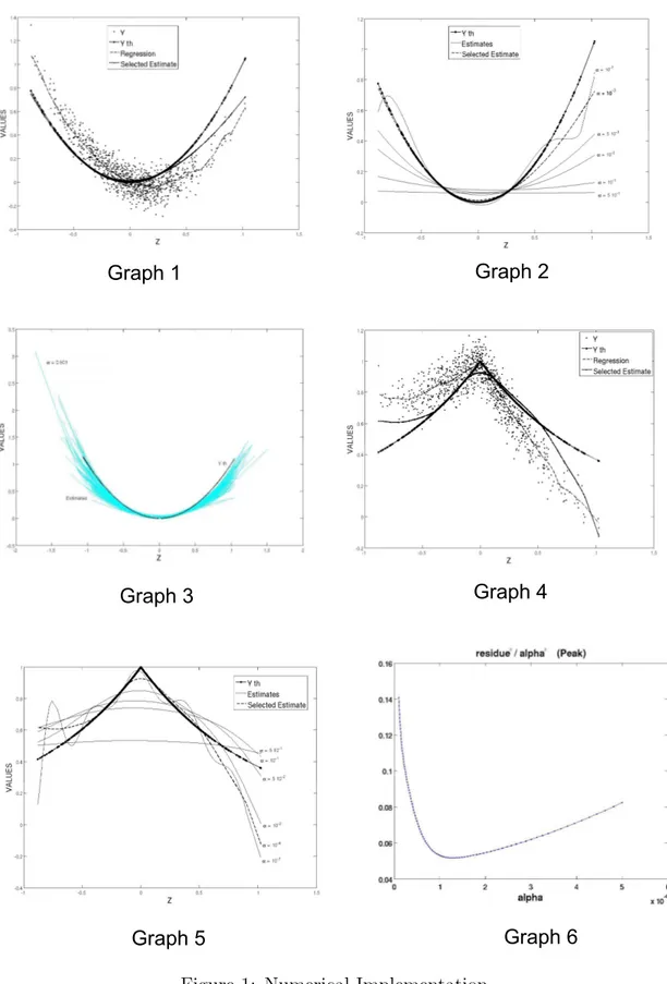
For ϕ (Z) = Z2, we present in Graph 1 the set of data (N = 1000) in the (Z, Y )
space, the true function, the kernel estimation of the regression and our estimation. In Graph 2, we show the evolution of our estimator for different values of αN and in
Graph 3 a Monte Carlo analysis is performed: a sample is generated 150 times and the estimation of ϕ is performed with the same bandwidths and same regularization parameter as in Graph 1. All these curves are plotted and give an illustration of
their distribution. Finally Graph 4 is identical to Graph 1 with ϕ (Z) = e−|Z| and
Graph 5 corresponds to Graph 2 in this case.
[Insert here Figure 1: Numerical Implementation]
Let us stress that the endogeneity bias in the estimation of the regression by kernel smoothing clearly appears. The estimated ϕ curve is not obviously related to the sample of Z and Y and depends on the instrumental variables W. Even though they cannot be represented, the instruments play a central role in the estimation.
The main question about the practical use of nonparametric instrumental vari-ables estimation is the selection of the bandwidth and of the αN parameter. This
question is complex and the construction of a data driven procedure for the simul-taneous selection of hN and αN is still an open question. We propose the following
sequential method:
i) Fix first the bandwidths for the estimation of r and of the joint density of Z
and W (for the estimation of T and T∗) by usual methods. Note that these
bandwidths do not need to be equal for the two estimations.
ii) Select αN by a data driven method. We suggest the following method based
on a residual approach extending the discrepancy principle of Morozov (1993). We consider the ”extended residuals” of the model defined by:
εαN = ˆT∗r − ˆˆ T∗T ˆˆϕαN
(2),
where ˆϕαN
(2) is the iterated Tikhonov estimation of order 2. Then:
To simplify the exposition, let’s assume h2ρN goes to zero at least as fast as 1/N. Then Assumption A.4 implies that the first term on the right hand side of the above displayed inequality is OP(√1N). Under the previous assumptions
it can be shown that k ˆT∗T ( ˆˆ ϕαN
(2) − ϕ)k2 = ° ° ° ° ³ ˆ T∗T ϕˆ ´αN (2) − ˆT ∗T ϕˆ ° ° ° ° 2 = OP(αN). This last property requires a regularization method of qualification at least 4 in order to characterize a β not greater than 2, and this is the motivation for the use of an iterated Tikhonov estimation at the first stage. Then we have:
1 α2 N kεαNk2 = O P( 1 α2 NN + α(β+2)∧4N ),
and a minimization with respect to αN of this value gives an αN with an
optimal speed (N−β+21 ) for the use in a non iterated Tikhonov estimation. In practice 1
α2
Nkε
αNk2 may be computed for different values of α
N and the
minimum can be selected. We give in Graph 6 this curve in the example of
ϕ(Z) = e−|Z|.
6
CONCLUSION
This paper has considered the nonparametric estimation of a regression function in presence of a simultaneity problem. We have established a set of general suffi-cient conditions to ensure consistency of our nonparametric instrumental variables estimator. The discussion of rates of convergence emphasizes the crucial role of the degree of ill-posedness of the inverse problem whose unique solution defines the regression function. A Monte Carlo illustration shows that our estimator is rather easy to implement and able to correct for the simultaneity bias displayed by the
naive kernel estimator. This paper treats essentially the purely nonparametric basic model and is in particular focused on kernel-based estimators. Numerous extensions are possible and relevant for the practical implementation of this procedure.
1. A first extension is to analyze the case where the explanatory variables Z con-tain exogenous variables also included in the instrumental variables W . These variables may be introduced in a nonparametric way or semi nonparametrically (ϕ(Z) becomes ϕ(Z) + X0β with X exogenous). In the general case, results
are essentially the same as in our paper by fixing these variables (see Hall and Horowitz (2005)). In the semi parametric case the procedure is described in Feve and Florens (2010).
2. The treatment of semi parametric models (additive, partially linear, index models,...) (see Florens, Johannes, and Van Bellegem (2005), Ai and Chen (2003)) or nonparametric models with constraints is helpful to reduce the curse of dimensionality.
3. We need to improve and to study more deeply the adaptive selection of the bandwidths and of the regularization parameter.
4. The structure L2 of the spaces may be modified. In particular Sobolev spaces
may be used and the penalty norm may incorporate the derivatives (see Gagliardini and Scaillet (2006), Blundell, Chen, and Christensen (2007)). This approach is naturally extended in terms of Hilbert scales (see Florens, Jo-hannes, and Van Bellegem (2007)).
5. Separable models may be extended to non separable models or more generally to non linear problems (duration models, auctions, GMM, dynamic models)
(see Ai and Chen (2003)).
6. A Bayesian approach to the nonparametric instrumental variables estimation (Florens and Simoni (2010)) enhances a use of gaussian process prior similar to machine learning.
7. In a preliminary version of this paper we give a proof of the asymptotic nor-mality of h bϕαN − ϕ, δi. This result is now presented in a separate paper.
APPENDIX A: PROOFS OF MAIN RESUTLS
PROOF OF PROPOSITION 2.1: i) ⇐⇒ ii): ii) implies i). Conversely, let us consider ϕ such that:
T∗T [ϕ (Z)] = E[E[ϕ (Z) | W ] | Z] = 0.
Then:
E£E[ϕ (Z) | W ]2¤= E[ϕ (Z) E[ϕ (Z) | W ]] = E[ϕ (Z) E[E[ϕ (Z) | W ] | Z]] = 0.
We obtain E[ϕ (Z) | W ] = 0 and ϕ = 0 using the strong identification condition.
i) ⇐⇒ iii): This property can be deduced from Florens, Mouchart, and Rolin
(1990), Theorem 5.4.3 or Luenberger (1969), Theorem 3, Section 6.3. Since R(T∗) =
N (T )⊥, R(T∗) = L2
F (Z) is tantamount to N (T ) = {0}. Q.E.D.
PROOF OF THEOREM 2.1: Let us first remark that: Z f2 Z,W1(z, w1) f2 Z(z) fW21(w1) fZ(z) fW1(w1)dzdw1 = Z ½Z fZ,W(z, w1, w2) fZ(z) fW(w1, w2) fW2|W1(w2 | w1)dw2 ¾2 fZ(z) fW1(w1)dzdw1 ≤ Z f2 Z,W(z, w1, w2) f2 Z(z) fW2 (w1, w2) fZ(z)fW(w1, w2)dzdw1dw2,
by Jensen’s inequality for conditional expectations. The first term is the Hilbert Schmidt norm of T∗
1T1 and the last one is the Hilbert Schmidt norm of T∗ T. Then
T∗
1T1 is an Hilbert Schmidt operator and
P
jλ2j,1 ≤
P
The eigenvalues may be compared pairwise. Using the Courant theorem (see Kress (1999), Theorem 15.14, page 276, Chapter 15), we get:
λ2j = min ρ0,ρ1,...,ρj−1∈L2z max kϕk=1 ϕ⊥(ρ0,ρ1,...,ρj−1) hT∗T ϕ, ϕi = max kϕk=1 ϕ⊥(ρ0,ρ1,...,ρj−1) kE (ϕ|w)k2 ≥ max kϕk=1 ϕ⊥(ρ0,ρ1,...,ρj−1) kE (ϕ|w1)k2 ≥ min ρ0,ρ1,...,ρj−1∈L2z max kϕk=1 ϕ⊥(ρ0,ρ1,...,ρj−1) T1∗T1ϕ, ϕ® = λ2j,1. Q.E.D.
PROOF OF THEOREM 4.1: The proof of Theorem 4.1 is based upon the de-composition: ˆ ϕαN − ϕ = A 1+ A2+ A3, with A1 = (αNI + ˆT∗T )ˆ −1Tˆ∗ˆr − (αNI + ˆT∗T )ˆ −1Tˆ∗T ϕˆ A2 = (αNI + ˆT∗T )ˆ −1Tˆ∗T ϕ − (αˆ NI + T∗T )−1T∗T ϕ A3 = (αNI + T∗T )−1T∗T ϕ − ϕ By Proposition 3.2: kA3k2 = O ³ αβ∧2N ´ ,
and, by virtue of Assumption A.4, we have directly: kA1k2 = OP · 1 α2 N µ 1 N + h 2ρ N ¶¸ .
To assess the order of A2, it is worth rewriting it as:
A2 = αN h (αNI + ˆT∗T )ˆ −1− (αNI + T∗T )−1 i ϕ = −αN(αNI + ˆT∗T )ˆ −1( ˆT∗T − Tˆ ∗T )(αNI + T∗T )−1ϕ = − (B1+ B2) , with B1 = αN(αNI + ˆT∗T )ˆ −1Tˆ∗( ˆT − T )(αNI + T∗T )−1ϕ B2 = αN(αNI + ˆT∗T )ˆ −1( ˆT∗− T∗)T (αNI + T∗T )−1ϕ By Assumption A.3: k ˆT − T k2 = OP µ 1 Nhp+qN + h 2ρ N ¶ , k ˆT∗− T∗k2 = OP µ 1 Nhp+qN + h 2ρ N ¶ , and, by Proposition 3.2: ° °αN(αNI + T∗T )−1ϕ ° °2 = O ³ αβ∧2N ´ , ° °αNT (αNI + T∗T )−1ϕ ° °2 = O ³ α(β+1)∧2N ´ ,
while ° ° °(αNI + ˆT∗T )ˆ −1Tˆ∗ ° ° °2 = OP µ 1 αN ¶ , ° ° °(αNI + ˆT∗T )ˆ −1 ° ° °2 = OP µ 1 α2 N ¶ . Therefore kA2k2 = OP "µ 1 Nhp+qN + h 2ρ N ¶ Ã αβ∧2N αN + α(β+1)∧2N α2 N !# = OP ·µ 1 Nhp+qN + h 2ρ N ¶ ³ α(β−1)∧1N + α(β−1)∧0N ´¸ = OP ·µ 1 Nhp+qN + h 2ρ N ¶ α(β−1)∧0N ¸ . Q.E.D.
APPENDIX B: VERIFICATION OF ASSUMPTIONS A.3 AND A.4
The objective of this appendix is to give a set of primitive conditions which imply the main assumptions of the paper for the kernel estimator. For notational compactness, in this appendix, we will suppress the subscripts in bfW (w), bfZ(z),
and bfZ,W(z, w) and the corresponding pdfs. They will be distinguished by their
arguments. We will also suppress the subscript in hN. We use C to denote a generic
positive constant which may take different values in different places and adopt the following assumptions.
ASSUMPTION B.1: (i) The data (yn, zn, wn), n = 1, ..., N , define an i.i.d
sam-ple of (Y, Z, W ); (ii) The pdf f (z, w) is d times continuously differentiable in the interior of [0, 1]p× [0, 1]q.
ASSUMPTION B.2: The pdf f (z, w) is bounded away from zero on the support [0, 1]p× [0, 1]q.
ASSUMPTION B.3: Both multivariate kernels KZ,h and KW,h are product
ker-nels generated from the univariate generalized kernel function Kh satisfying: (i) the
kernel function Kh(·, ·) is a generalized kernel function of order l; (ii) for each
t ∈ [0, 1], the function Kh(h·, t) is supported on [(t − 1) /h, t/h] ∩ K, where K is a
compact interval not depending on t and:
sup
h>0,t∈[0,1],u∈K
|Kh(hu, t)| < ∞.
ASSUMPTION B.4: The smoothing parameter satisfies: h → 0 and (Nhp+q)−1log N → 0.
The independence assumption is a simplifying assumption and could be extended to weakly dependent (stationary mixing) observations. Assumption B.3 is the same as A.5 in Hall and Horowitz (2005). We first provide a result on the uniform con-vergence of bf (w), bf (z), and bf (z, w) with rates. For density functions with compact
support, uniform convergence of kernel density estimators using ordinary kernel functions must be restricted to a proper subset of the compact support. Using gen-eralized kernel functions, we show uniform convergence over the entire support. A similar result is provided in Proposition 2 (ii) in Rothe (2009). However, the as-sumptions in Rothe (2009) differ from our asas-sumptions and no proof is provided in Rothe (2009).
LEMMA B.1: Suppose Assumptions B.1-B.4 hold. Let ρ = min {l, d}. Then:
(i) sup w∈[0,1]q ¯ ¯ ¯ bf (w) − f (w) ¯ ¯ ¯ = OP ³£ (Nhq)−1log N¤1/2+ hρ ´ = oP (1) ; (ii) sup z∈[0,1]p,w∈[0,1]q ¯ ¯ ¯ bf (z, w) − f (z, w) ¯ ¯ ¯ = OP µh¡ Nhp+q¢−1log Ni1/2+ hρ ¶ = oP (1) ; (iii) sup z∈[0,1]p ¯ ¯ ¯ bf (z) − f (z) ¯ ¯ ¯ = OP ³£ (Nhp)−1log N¤1/2+ hρ´= o P (1) .
PROOF OF LEMMA B.1: We provide a proof of (i) only. First we evaluate the bias of bf (w). Let w = (w1, ..., wq)0. Then:
E ³ b f (w) ´ = 1 hqE [KW,h(w − wn, w)] = 1 hq Z [0,1]q KW,h(w − v, w)f (v) dv = Z Πqj=1hwj −1h ,wjhi KW,h(hv, w)f (w − hv) dv = Z Πqj=1hwj −1h ,wjhi KW,h(hv, w) f (w) + (−h) Pq j=1 ∂f (w) ∂wj vj + · · · +1 ρ! Pq j1=1· · · Pq jρ=1 ∂ρf (w∗) ∂wj1···∂wjρ (−h) ρv j1· · · vjρ dv,
where w∗ lies between w and (w − hv). Now making use of Assumptions B.2-B.4,
we get: sup w∈[0,1]q ¯ ¯ ¯E ³ b f (w) ´ − f (w) ¯ ¯ ¯ ≤ Chρ " sup h>0,t∈[0,1],u∈K |Kh(hu, t)| #q = O (hρ) .
It remains to show: supw∈[0,1]q ¯ ¯ ¯ bf (w) − E h b f (w) i¯¯ ¯ = OP ³£ (Nhq)−1log N¤1/2´. This
can be shown by the standard arguments in the proof of uniform consistency of kernel density estimators based on ordinary kernel functions, see e.g., Hansen (2008) and references therein. Q.E.D.
The next lemma shows that Assumption A.3 is satisfied under the previous conditions. Actually, this lemma proves a stronger result as the one needed for Assumption A.3 because the convergence is proved in Hilbert Schmidt norm which implies the convergence for the supremum norm.
LEMMA B.2: Suppose Assumptions B.1-B.4 hold. Then: (i) ° ° ° bT − T ° ° °2 HS = OP ³ (Nhp+q)−1+ h2ρ´, (ii) ° ° ° bT∗− T∗°°°2 HS = OP ³ (Nhp+q)−1+ h2ρ´,
where k·kHS denotes the Hilbert-Schmidt norm, i.e.,
° ° ° bT − T ° ° °2 HS = Z [0,1]q Z [0,1]p h b f (z|w) − f (z|w)i2 f2(z) f (z) f (w) dzdw = Z [0,1]q Z [0,1]p " b f (z, w) b f (w) − f (z, w) f (w) #2 f (w) f (z)dzdw.
PROOF OF LEMMA B.2 (i): Let R R · dzdw =R[0,1]q R [0,1]p· dzdw. Note that: ° ° ° bT − T ° ° °2 HS =Z Z " bf (z, w) b f (w) − f (z, w) f (w) #2 f (w) f (z)dzdw =Z Z " bf (z, w) f (w) − f (z, w) bf (w) b f (w) f (w) #2 f (w) f (z)dzdw ≤ 1 infw∈[0,1]q h b f (w) i2 Z Z " bf (z, w) f (w) − f (z, w) bf (w) f (w) #2 f (w) f (z)dzdw = OP (1) Z Z bf (z, w) − f (z, w) − f (z, w) h b f (w) − f (w) i f (w) 2 f (w) f (z)dzdw = OP (1) Z Z hf (z, w) − f (z, w)b i2 f (z) f (w) dzdw + OP (1) Z Z f2(z, w)hf (w) − f (w)b i2 f (w) f (z) dzdw ≡ OP (1) (A1+ A2) ,
where we have used the fact that 1 infw∈[0,1]q[f (w)b ]
2 = OP(1) implied by Assumptions
B.2, B.4, and Lemma B.1. Now, we show:
A1 = OP ³¡ Nhp+q¢−1+ h2ρ ´ and A2 = OP ¡ (Nhq)−1+ h2ρ¢. As a result, we obtain ° ° ° bT − T ° ° °2 HS = OP ³ (Nhp+q)−1+ h2ρ´.
We prove the result for A1. Note that:
E (|A1|) = Z Z Ehf (z, w) − f (z, w)b i2 f (z) f (w) dzdw = Z Z V ar ³ b f (z, w)´ f (w) f (z)dzdw + Z Z h E ³ b f (z, w) ´ − f (z, w) i2 f (w) f (z)dzdw = O³¡Nhp+q¢−1 ´ + O¡h2ρ¢.
This follows from the standard arguments for evaluating the first term and the proof of Lemma B.1 for the second term. By Markov inequality, we obtain A1 =
OP
³
(Nhp+q)−1+ h2ρ´. Q.E.D.
The next lemma shows that Assumption A.4 is satisfied under the primitive conditions.
LEMMA B.3: Suppose Assumptions B.1-B.4 hold. In addition, we assume
E (U2|W = w) is uniformly bounded in w ∈ [0, 1]q. Then:
° ° ° bT∗br − bT∗T ϕb ° ° °2 = OP (N−1+ h2ρ).
PROOF OF LEMMA B.3: By definition: ³ b T∗br − bT∗T ϕb ´ (z) = h b T∗ ³ b r − bT ϕ ´i (z) = Z ³ b r − bT ϕ ´ (w)f (z, w)b b f (z) dw = Z Ã b r (w) − Z ϕ (z0)f (zb 0, w) b f (w) dz 0 ! b f (z, w) b f (z) dw = Z Ã 1 Nhq N X n=1 ynKW,h(w − wn, w) − Z ϕ (z0) bf (z0, w)dz0 ! b f (z, w) b f (z) bf (w)dw ≡ Z AN(w) b f (z, w) b f (z) bf (w)dw.
Similar to the proof of Lemma B.2, we can show by using Lemma B.1 that uniformly in z ∈ [0, 1]p, the following holds:
³ b T∗br − bT∗T ϕb ´ (z) = Z AN (w) f (z, w) f (z)f (w)dw + oP µZ AN(w) f (z, w) f (z)f (w)dw ¶ .
Thus, it suffices to show that ° ° °R AN(w)f (z)f (w)f (z,w) dw ° ° °2 = OP(N−1+ h2ρ). Writing AN(w) as: AN(w) = 1 Nhq N X n=1 UnKW,h(w − wn, w) + 1 Nhq N X n=1 · ϕ (zn) − 1 hp Z ϕ (z0) K Z,h(z0− zn, z0)dz0 ¸ KW,h(w − wn, w) ≡ AN 1(w) + AN 2(w) ,
we obtain: E "° ° ° ° Z AN(w) f (z, w) f (z)f (w)dw ° ° ° ° 2# ≤ 2E "° ° ° ° Z AN 1(w) f (z, w) f (z)f (w)dw ° ° ° ° 2 + ° ° ° ° Z AN 2(w) f (z, w) f (z)f (w)dw ° ° ° ° 2# = 2 Z Z Z E [AN 1(w) AN 1(w0)] f (z, w)f (z, w0) f (z)f (w)f (w0)dwdw 0dz + 2 Z Z Z E [AN 2(w) AN 2(w0)] f (z, w)f (z, w0) f (z)f (w)f (w0)dwdw 0dz = 2BN 1+ 2BN 2.
Below, we will show that BN 1 = O (N−1) and BN 2= O (N−1+ h2ρ). First consider
the term BN 1: BN 1 = 1 Nh2q Z Z Z E£Un2KW,h(w − wn, w)KW,h(w0− wn, w0) ¤ f(z, w)f (z, w0) f (z)f (w)f (w0)dwdw 0dz = 1 N Z E R(1−wn)/h −wn/h R(1−wn)/h −wn/h U 2 nKW,h(hw, wn+ hw)KW,h(hw0, wn+ hw0) f (z,wn+hw)f (z,wn+hw0) f (z)f (wn+hw)f (wn+hw0)dwdw 0 dz ≤ CN−1 " sup h>0,t∈[0,1],u∈K |Kh(hu, t)| #2q = O¡N−1¢,
Now for BN 2, letting B (zn) = ϕ (zn) − h1p R ϕ (z0) K Z,h(z0− zn, z0)dz0, we get: BN 2 = 1 (NhqN)2 X X n6=n0 Z Z Z E [B (zn) KW,h(w − wn, w)] E [B (zn0) KW,h(w0 − wn0, w0)]f (z, w)f (z, w 0) f (z)f (w)f (w0)dwdw 0dz + 1 Nh2q Z Z Z E£[B (zn)]2KW,h(w − wn, w)KW,h(w0− wn, w0) ¤ f(z, w)f (z, w0) f (z)f (w)f (w0)dwdw 0dz = 1 (Nhq)2 X X n6=n0 Z ·Z E [B (zn) KW,h(w − wn, w)] f (z, w) f (w) dw ¸2 1 f (z)dz + 1 Nh2q Z Z Z E£[B (zn)]2KW,h(w − wn, w)KW,h(w0− wn0, w0)¤ f(z, w)f (z, w 0) f (z)f (w)f (w0)dwdw 0dz = 1 (Nhq)2 X X n6=n0 Z ·Z E [B (zn) KW,h(w − wn, w)] f (z, w) f (w) dw ¸2 1 f (z)dz + O¡N−1¢,
where the second term on the right hand side of the second last equation can be shown to be O (N−1) by change of variables and by using Assumptions B.1-B.4. Let
BN 21 denote the first term, i.e.,
BN 21 = 1 (Nhq)2 X X n6=n0 Z ·Z E [B (zn) KW,h(w − wn, w)] f (z, w) f (w) dw ¸2 1 f (z)dz.
Then it suffices to show that BN 21 = O(h2ρ). Similar to the proof of Lemma B.1,
we note that, uniformly in z ∈ [0, 1]p, we get: 1 hq Z E [B (zn) KW,h(w − wn, w)]f (z, w) f (w) dw = 1 hq Z E [ϕ (zn) KW,h(w − wn, w)] f (z, w) f (w) dw − Z Z ϕ (z0) E · 1 hp+qKZ,h(z 0− z n, z0)KW,h(w − wn, w) ¸ dz0f (z, w) f (w) dw = O¡h2ρ¢. As a result, we obtain BN 1 + BN 2 = O (N−1+ h2ρ) or E ·° ° ° bT∗br − bT∗T ϕb °°°2 ¸ =
References
Ai, C., and X. Chen (2003): Efficient Estimation of Conditional Moment Re-strictions Models Containing Unknown Functions, Econometrica, 71, 1795-1843. Basu, D. (1955): On Statistics Independent of a Sufficient Statistic, Sankhya, 15, 377-380.
Blundell, R., X. Chen, and D. Kristensen (2007): Semi-Nonparametric IV Estimation of Shape-Invariant Engel Curves, Econometrica, 75, 1613-1669. Blundell, R., and J. Horowitz (2007): A Non Parametric Test of Exogeneity, Review of Economic Studies, 74, 1035-1058.
Carrasco, M., and J.P. Florens (2000): Generalization of GMM to a Continuum of Moment Conditions, Econometric Theory, 16, 797-834.
Carrasco, M., and J.P. Florens (2009): Spectral Method for Deconvolving a Density, forthcoming Econometric Theory.
Carrasco, M., J.P. Florens, and E. Renault (2007): Linear Inverse Problems, in Structural Econometrics: Estimation Based on Spectral Decomposition and Regularization, ed. by J. Heckman and E. Leamer. Elsevier, North Holland, 5633-5751.
Chen, X., and M. Reiss (2007): On Rate Optimality for Ill-posed Inverse Problems in Econometrics, forthcoming Econometric Theory.
Darolles, S., J.P. Florens, and E. Renault (1998): Nonlinear Principal Com-ponents and Inference on a Conditional Expectation Operator, Unpublished Manuscript, CREST.
Engl, H.W., M. Hanke, and A. Neubauer (2000): Regularization of Inverse Problems. Springer, Netherlands.
Feve, F., and J.P. Florens (2010): The Practice of Nonparametric Estimation by Solving Inverse Problem: The Example of Transformation Models, The Econometric Journal, 13, 1-27.
Florens, J.P. (2003): Inverse Problems and Structural Econometrics: The Example of Instrumental Variables, in Advances in Economics and Economet-rics: Theory and Applications, ed. by M. Dewatripont, L.P. Hansen and S.J. Turnovsky. Cambridge University Press, 284-311.
Florens, J.P. (2005): Endogeneity in Non Separable Models. Application to Treat-ment Effect Models where Outcomes are Durations, Unpublished Manuscript, Toulouse School of Economics.
Florens, J.P., J. Heckman, C. Meghir, and E. Vytlacil (2008): Identification of Treatment Effects using Control Function in Model with Continuous Endogenous Treatment and Heterogenous Effects, Econometrica, 76, 1191-1206.
Florens, J.P., J. Johannes, and S. Van Bellegem (2005): Instrumental Regression in Partially Linear Models, forthcoming Econometric Journal.
Florens, J.P., J. Johannes, and S. Van Bellegem (2007): Identification and Esti-mation by Penalization in Nonparametric Instrumental Regression, forthcoming Econometric Theory.
Florens, J.P., and M. Mouchart (1986): Exhaustivite, Ancillarite et Identification en Statistique Bayesienne, Annales d’Economie et de Statistique, 4, 63-93. Florens, J.P., M. Mouchart, and J. M. Rolin (1990): Elements of Bayesian Statistics. Dekker, New York.
Florens, J.P., M. Mouchart, and J. M. Rolin (1993): Noncausality and Marginal-ization of Markov Process, Econometric Theory, 9, 241-262.
Instrumen-tal Variables Regression : a Quasi Bayesian Approach Based on a Regularized Posterior, forthcoming Journal of Econometrics.
Gagliardini, C., and O. Scaillet (2006): Tikhonov regularisation for Functional Minimum Distance Estimators, Unpublished Manuscript, Swiss Finance Insti-tute.
Gavin, J., S. Haberman, and R. Verall (1995): Graduation by Kernel and Adaptive Kernel Methods with a Boundary Correction, Transaction of Society of Actuaries, 47, 173-209.
Groetsch, C. (1984): The Theory of Tikhonov Regularization for Fredholm Equations of the First Kind. Pitman, London.
Hall, P., and J. Horowitz (2005): Nonparametric Methods for Inference in the Presence of Instrumental Variables, Annals of Statistics, 33, 2904-2929.
Hall, P., and J. Horowitz (2007): Methodology and Convergence Rates for Functional Linear Regression, Annals of Statistics, 35, 70-91.
Hansen, B. E. (2008): Uniform Convergence Rates for Kernel Estimation With Dependent Data, Econometric Theory, 24, 726-748.
Hardle, W., and O. Linton (1994): Applied Nonparametric Methods, in Hand-book of Econometrics, ed. by R.F. Engle and D.L. McFadden. Elsevier, North Holland, 2295-2339.
Horowitz, J. (2006): Testing a Parametric Model Against a Nonparametric Alternative with Identification through Instrumental Variables, Econometrica, 74, 521-538.
Horowitz, J., and S. Lee (2007): Non parametric Instrumental Variables Estima-tion of a Quantile Regression Model, Econometrica, 75, 1191-1208.