L A B O R A T O I R E D ’ A N A L Y E T M O D É L I S A T I O N S Y S T È M E S P O U R L ’ A I D E L A D É C I S I O N U N I T É E C H E R C H E A S S O C I É E C N U 7 0 2 4 U N I V E R S I T É P A R I S S E D E À D E R S M R D A U P H I N E P L A C E D U Ma l D E L A T T R E D E T A S S I G N Y F - 7 5 7 7 5 P A R I S C E D 1 6 T É L É P H O N E ( 3 3 1 ) ( 0 4 4 0 5 4 4 6 6 T É L É C O P I E ( 1 ) ( 0 1 ) 4 4 0 5 4 0 9 1 E - M A E X 1 ) 3 3 I L r o -c h e @ l a m s a d e . d a u p h i n e . f r W E B w w w . l a m s a d e . d a u p h i n e . f r
On the Complexity of Global Constraint Satisfaction
NOTE N° 38
C. Bazgan, M. Karpinski (1)
juin
2005
(1) CNRS- LAMSADE, Université Paris-Dauphine, Place du Maréchal De
Lat-tre de Tassigny, 75775 Paris Cedex 16.
On the Complexity of Global Constraint Satisfaction
Cristina Bazgan∗ Marek Karpinski†
June 22, 2005
Abstract
We study the computational complexity of decision and optimization problems that may be expressed as boolean contraint satisfaction problem with the global cardinality constraints. In this paper we establish a characterization theorem for the decision prob-lems and derive approximation hardness results for the corresponding global optimization problems.
1
Introduction
Constraints of the global nature arise naturally in some optimization problems. For example, Min Bisection can be viewed as Min Cut with the restriction that the two sets of vertices that determine the cut must be of equal size. It is known that Min Cut is polynomial while Min Bisection is NP -hard. Min Bisection, Max Bisection and other optimization problems can be written as boolean constraint satisfaction problems where a feasible solution is a balanced assignment (where the number of variables set to 1 is the same as the number of variables set to 0). It was an increased interest in global optimization problems recently, cf. [HZ01, FL01, JS04].
In this paper we study the complexity of decision and optimization problems of the bal-anced versions of boolean constraint satisfaction problems depending on the type of con-straints. Schaefer [Sch78] established a dichotomy theorem for the boolean constraint satis-faction problems distinguishing six polynomial time solvable cases. For the decision versions we show that if the set of constraints contains only equations of width 2 or it contains only conjunctions of literals, then the balanced version is polynomial time solvable and otherwise it is NP -complete.
Creigou [Cre95] and Khanna and Sudan [KS96] established a dichotomy theorem for max-imization versions of boolean constraint satisfaction problems that classify the problems into polynomially solvable or APX -hard. The balanced versions of these problems where also stud-ied. Sviridenko [Svi01] proved that the balanced version of Max Sat is 1/(1−1e)-approximable.
∗LAMSADE, Université Paris-Dauphine, 75775 Paris, [email protected]. Research supported
by DAAD.
For the balanced version of Max 2Sat, Blaser and Manthey [BM02] established a 1.514-approximation factor and Hofmeister [Hof03] a 4/3-1.514-approximation factor. Lower bound were also studied for these problems. Holmerin [Hol02] showed that the balanced version of Max E4-0H-Lin2 (see for the definition Section 2) cannot be approximated within 1.0957 in poly-nomial time, unless P =NP. Also Holmerin and Khot [HK03] showed that balanced version of Max E3-0H-Lin2 is hard to approximate within 43 − ε and in [HK04] they improved their result showing that this problem is hard to approximate within 2 − ε, for any ε > 0, if NP 6⊆ ∩δ>0 DTIME (2n
δ
), thus obtaining the best possible inapproximability factor result for this problem. We prove in this paper that all the cases that were considered by Creigou [Cre95] and Khanna and Sudan [KS96] in the dichotomy theorem become APX -hard and also that most of the trivial maximization constraint satisfaction problems have their balanced version APX -hard. In particular, using an inapproximability result for Densest k Subgraph established recently by Khot [Kho04], we prove that the balanced version of Min Monotone-E2Sat has no polynomial time approximation scheme, if NP 6⊆ ∩δ>0 BTIME (2n
δ
), for BTIME denoting randomized polynomial time.
Khanna, Sudan and Trevisan [KST97] established a classification theorem for minimization versions of boolean constraint satisfaction problems. The complexity of approximation of Min Bisection was for long time widely open. Feige and Krautghamer [FK00] established an approximation algorithm for this problem within O(log2n) approximation factor. This result has been recently improved to O(log1.5n) by the recent result of Arora, Rao and Vazirani [ARV04]. Very recently, Khot [Kho04] established that under the assumption that NP 6⊆ ∩δ>0
BTIME (2nδ), Min Bisection has no polynomial time approximation scheme. Under the
assumption that refuting SAT formulas is hard to approximate on average, Feige [Fei02] proved also that Min Bisection is hard to approximate below 43.
Holmerin studied the hardness of approximating some generalizations of Min Bisec-tion. In particular he showed [Hol02] that the balanced version of Min E4-1H-Lin2 is not (2 − ε)-approximable for any ε > 0, unless P=NP. We prove several inapproximability result for balanced minimization problem. In particular, using the inapproximability result for Densest k Subgraph established by Khot [Kho04], we prove that the balanced version
of Min Monotone-E2Sat has no polynomial time approximation scheme, if NP 6⊆ ∩δ>0
BTIME (2nδ
).
The paper is organized as follows: in Section 2 we introduce some preliminary notation and definitions, Section 3 contains our results on decision problems and Section 4 contains a summary of these results.
In Section 5 and 6 we present our results concerning maximization and minimization optimization problems. In Section 7 we summarize chains of reductions preserving the ap-proximation and in Section 8 we briefly consider dense instances of the problems considered in the chains of reductions. Section 9 contains some open questions.
2
Preliminaries
We refer a general reader to [KST97, KSW97, KSTW01, CKS01] for a background on the boolean constraint satisfaction problems.
A constraint is a boolean function f : {0, 1}k → {0, 1}. A constraint application is a pair < f, (i1, . . . , ir) > where r is the arity of f and the i` ∈ [n] indicate to which r of the n
boolean variables a given constraint is applied. This constraint application will be denoted in the following by f (xi1, . . . , xir).
Let F = {f1, . . . , ft} be a finite collection of boolean functions. An F-set of constraints on
n boolean variables x1, . . . , xn is a collection of constraint applications {fj(xj1, . . . , xjrj)}
m j=1
for some integer m, where fj ∈ F and rj is the arity of fj. We say that an assignment satisfies
an F-set of constraints if it satisfies every constraint in the collection.
The satisfiability problem CSP(F) consists of deciding whether there exists an assignment that satisfies a given F-set of constraints.
kCSP(F) (respectively, EkCSP(F)) is the variant of CSP(F) where each boolean func-tion fj is a function of at most (respectively, exactly) k variables, for j ≤ t. The problems
Max (Min) CSP(F) consist of finding a boolean assignment that maximizes (minimizes) the number of constraints that are satisfied. Max (Min) kCSP(F) (respectively, Max (Min) EkCSP(F)) are variants of Max (Min) CSP(F) where each constraint depends on at most (respectively, exactly) k literals.
Given a problem A, the Balanced version of A is the problem A with a new set of feasible solutions being assignments where the number of variables set to true (denoted by 1) is the same as the number of variables set to f alse (denoted by 0). Such assignments will be called balanced assignments.
We consider also a generalization of this problem. Given a problem A, the α-Balanced version of A, 0 < α < 1, is the problem A with a new set of feasible solutions being assignments with the number of true variables being an α ratio of the total number of variables. Such assignments will be called in the following α-balanced.
In this paper we study the complexity of decision and optimization problems related to Balanced CSP(F) depending on the type of constraints defined by a class F.
We start by defining the types of constraints studied in this paper. A boolean function f will be called
• 0-valid if f(0, . . . , 0) = 1. • 1-valid if f(1, . . . , 1) = 1.
• weakly negative (Horn) if f is expressible as a CNF-formula having at most one un-negated variable in each clause.
• weakly positive (anti-Horn) if f is expressible as a CNF-formula having at most one negated variable in each clause.
• affine if f is expressible as a conjunction of linear equations over GF (2) and affine with width 2 if each equation depend on 2 variables.
• 2-monotone if f is expressible as a DNF of the type xi1∧ . . . ∧ xip or ¯xj1 ∧ . . . ∧ ¯xjq or
(xi1 ∧ . . . ∧ xip) ∨ (¯xj1 ∧ . . . ∧ ¯xjq).
In the following we give definitions of the problems that we consider in this paper. kSat (respectively, EkSat) is the version of Sat where each clause is of size at most (respectively, exactly) k. kSat (B, ¯B) is the variant of kSat where each literal appears at most B times. Monotone-EkSat is the variant of the EkSat problem where either all clauses contain only positive literals or all clauses contain only negative literals.
In this paper we use the notation AND instead of DNF for the problem of deciding whether a set of conjunctions of literals has a satisfiable assignment. Monotone-EkAND is the variant of the EkAND problem where either all conjunctions contain only positive literals or they contain only negative literals.
The input of the EkLin2 problem is a set of equations of the type xi1 ⊕ . . . ⊕ xik = 0
or xi1 ⊕ . . . ⊕ xik = 1, and we have to decide if there is a satisfiable assignment. In the
homogenous variants of linear equations problem, Ek-bH-Lin2, b ∈ {0, 1}, the input consists of a set of equations of the type xi1⊕ . . . ⊕ xik = b on n boolean variables x1, . . . , xn and the
problem consists of deciding if there is an assignment satisfying all equations.
Max kSat is the problem, given a set of clauses, of constructing an assignment satisfying a maximum number of clauses.
Max kAND is the problem, given a set of conjunctions of size at most k, of determining an assignment maximizing the number of conjunctions satisfied.
Max EkLin2 is the problem, given a set of equations mod 2, of constructing an assignment maximizing the number of equations satisfied.
Min kSat is the problem, given a set of clauses, of constructing an assignment satisfying a minimum number of clauses.
Min kAND is the problem, given a set of conjunctions of size at most k, of determining an assignment minimizing the number of conjunctions satisfied.
Min EkLin2 is the problem, given a set of equations mod 2, of constructing an assignment minimizing the number of equations satisfied.
We give now some basic notions on approximation complexity of optimization problems. Given an NPO optimization problem ([ACG+99]) A and an instance I of A, we use |I| to denote the size of I, opt(I) to denote the optimum value for this instance and val(I, S) to denote the value of a feasible solution S of instance I. The performance ratio of S (or approximation factor) is r(I, S) = maxnval(I,S)opt(I) ,val(I,S)opt(I) o. The error of S, ε(I, S), is defined by ε(I, S) = r(I, S) − 1.
For a function f , an algorithm A is an f (n)-approximation, if for every instance I of the problem A, it returns a solution S such that r(I, S) ≤ f(|I|). For a constant c, an algorithm A is a (randomized) c-approximation, if for any instance I of the problem, it returns a solution S such that r(I, S) ≤ c. We say that an optimization problem is constant factor approximable if, for some constant c, there exists a polynomial time c-approximation algorithm for it. The class of problems which are constant factor approximable is denoted by AP X.
The notion of an E-reduction (error-preserving reduction), denoted here by ≤, was in-troduced by Khanna, Motwani, Sudan and Vazirani in [KMSV94]. A problem A is called E-reducible to a problem B, if there exist polynomial time computable functions f , g and a constant β such that
• f maps an instance I of A to an instance I0 of B such that opt(I) and opt(I0) are
related by a polynomial factor, i.e. there exists a polynomial p(n) such that opt(I0) ≤
p(|I|)opt(I),
• g maps solutions S0 of I0 to solutions S of I such that ε(I, S) ≤ βε(I0, S0).
An important property of that reduction is that it can be applied uniformly to all levels of approximability; that is, if A is E-reducible to B and B belongs to C then A belongs to C as well, where C is a class of optimization problems with any kind of approximation guarantee (see also [KMSV94]).
We call two optimization problems A and B, E-equivalent if A ≤ B and B ≤ A.
A problem A is AP X-hard, if every problem B ∈ AP X is such that B ≤ A. A problem is called AP X-complete if it belongs to AP X, and it is AP X-hard.
We formulate our results in terms of E-reductions (note that some authors use, say for min-imization problems, different kind of reductions [KSTW01, CP91]). Given two optmin-imization problems A and B we say that B is A-complete if A is E-reducible to B, and vice versa.
3
Complexity of Decision Problems
The decision complexity of boolean constraint satisfaction problems is well established. In particular, Schaefer [Sch78] established the following remarkable dichotomy theorem:
Theorem 1 (Dichotomy Theorem for CSP(F) [Sch78]) Given an F-set of constraints, the problem CSP(F) is polynomial time computable if F satisfies one of the conditions below, and CSP(F) is NP-complete otherwise.
1. Every function in F is 0-valid. 2. Every function in F is 1-valid.
3. Every function in F is weakly positive. 4. Every function in F is weakly negative. 5. Every function in F is affine.
6. Every function in F is bijunctive.
Motivated by the above result, we aim at formulating analogous result for balanced prob-lems. Firstly we show that for any F-set of constraints, Balanced CSP(F) is at least as difficult as CSP(F).
Proof : We reduce CSP(F) to Balanced CSP(F). Given an instance I of CSP(F) on n variables x1, . . . , xn and with m constraints, we construct an instance I0 of Balanced
CSP(F) on 2n variables x1, . . . , xn and n new variables y1, . . . , yn. For each constraint
fj(xj1, . . . , xjrj) of I we add to I
0the following two constraints: f
j(xj1, . . . , xjrj) and fj(¯yj1, . . . ,
¯
yjrj). It is easy to see that if xi = vi, i = 1, . . . , n is an assignment that satisfies I then
xi = vi, yi = ¯vi, i = 1, . . . , n is a balanced assignment that satisfies I0, where ¯v means the
complemented value of v. Conversely, if xi = vi, yi = wi, i = 1, . . . , n is a balanced assignment
that satisfies I0 then x
i = vi, i = 1, . . . , n is an assignment that satisfies I. 2
We turn now to a polynomial time case. We formulate our result in slightly more general setting of the α-balanced problems.
Theorem 2 For any 0 < α < 1, α-Balanced E2-Lin2 is solvable in polynomial time. Proof : Let us consider first α = 12. Given an instance I of Balanced E2-Lin2 on n variables and m equations, we construct some equivalence classes on the set of literals by considering the equations one after another as follows. Given an equation xi⊕ xj = 0 (xi⊕ xj=1), we
distinguish the following cases.
• If literals xi, ¯xi, xj, ¯xj do not appear in a class, then we construct a new class and we
put together xi and xj (xi and ¯xj respectively).
• If either xi or ¯xi appears in a class Ck and xj, ¯xj do not appear in a class, then
– if xi ∈ Ck then we introduce xj (¯xj respectively) in Ck.
– if ¯xi ∈ Ck then we introduce ¯xj (xj respectively) in Ck.
• If literals xi or ¯xi and xj or ¯xj appear in the same class Ck then I is not satisfiable if
{xi, ¯xj} ⊆ Ck or {¯xi, xj} ⊆ Ck ({xi, xj} ⊆ Ck or {¯xi, ¯xj} ⊆ Ck respectively).
• If either xi or ¯xi appears in a class Ck and either xj or ¯xj appears in a class C` then
– if xi ∈ Ck and xj ∈ C` then we put together the literals of both classes Ck and C`
(we put together the literals of the class Ck with the negated literals of the class
C`).
– if xi ∈ Ck and ¯xj ∈ C` then we put together the literals of the class Ck with the
negated literals of the class C` (we put together the literals of both classes Ck and
C`).
Suppose that at the end we obtain t equivalence classes C1, . . . , Ct. Denote by a2i−1 and
a2i the number of literals that appear positive and respectively negative in Ci. Balanced
E2-Lin2 on I consists of deciding if there exists a partition of these 2t integers in two equal size sets P and N such that P and N contain exactly one of a2i−1, a2i for i = 1, . . . , t. This
problem in solvable in polynomial time by dynamic programming [GJ76]. If such a partition P , N exists then the following assignment is balanced and satisfies I:
• if a2i−1∈ P then we assign to the positive variables of Ci the value 1 and to the negated
• if a2i−1∈ N then we assign to the positive variables of Ci the value 0 and to the negated
variables of Ci the value 1.
If α 6= 12 then as below we construct equivalence classes C1, . . . , Ct and compute integers
a1, . . . , a2t. We add two other integers a2t+1 = n|1 − 2α|, a2t+2 = 0 and solve the above
partition problem on this new instance. 2
Before we attack the "Ek"-situation for k ≥ 3, we establish some auxiliary results. Proposition 1 Balanced Ek-0H-Lin2 and Balanced Ek-1H-Lin2 are polynomial equiv-alent, for every odd k ≥ 3.
Proof : We reduce Balanced Ek-0H-Lin2 to Balanced Ek-1H-Lin2. From an instance I of Balanced Ek-0H-Lin2 on n variables x1, . . . , xn we construct an instance I0 on the
same set of variables and we associate to each equation xi1⊕ . . . ⊕ xik = 0 of I the equation
xi1 ⊕ . . . ⊕ xik = 1 in I
0. It is easy to see, since k is odd, an assignment satisfies I if and only
if the complemented assignment satisfies I0. The reduction in the other direction is similar. 2
We define a new problem to be used later. kOnes(E3-bH-Lin2), b ∈ {0, 1}
Input: A set of equations of the type xi1 ⊕ xi2⊕ xi3 = b on n boolean variables x1, . . . , xn.
Question: Is there an assignment, with exactly k variables set to 1, satisfying all equations ? Max Ones(F) consists of determining an assignment that satisfies all constraints of F-type and maximizes the number of variables assigned to 1.
Theorem 3 ([KSW97, KSTW01]) If every function in F is of the type xi1⊕ xi2⊕ xi3 = 0
or if every function in F is of the type xi1⊕ xi2⊕ xi3 = 1 then the problem Max Ones(F) is
APX-complete.
A consequence of the previous theorem is that kOnes(E3-0H-Lin2) and kOnes(E3-1H-Lin2) are NP -complete.
Proposition 2 Balanced E3-0H-Lin2 and Balanced E3-1H-Lin2 are both NP-complete.
Proof : We construct a reduction between kOnes(Lin2) and Balanced
E3-0H-Lin2. Given an instance I of kOnes(E3-0H-Lin2) on n variables x1, . . . , xnwe construct an
instance I0 on 2n variables x
1, . . . , xn, y1, . . . , yn−k, z1, . . . , zk as follows. For each equation
xi1 ⊕ xi2 ⊕ xi3 = 0 from I, we associate in I
0 the same equation and let us denote in the
following this set of equations by A. We add also to I0 the following set of equations, called
B, yi ⊕ yj ⊕ z` = 0 for every i, j ∈ {1, . . . , n − k}, ` ∈ {1, . . . , k}, i 6= j. It is easy to see
that in order that an assignment satisfies B the variables y must have the same value and the variables z must have the same value. Thus, an assignment that satisfies B has zi = 0,
i = 1, . . . , k. Suppose that yi = 0, i = 1, . . . , n −k then since the assignment must be balanced
we have xi = 1, i = 1, . . . , n but in this case the equations in A are not satisfied. So, yi = 1,
i = 1, . . . , n − k and due to the balanced condition, the restriction of this assignment to variables x satisfies I and contains exactly k variables 1 and n − k variables 0. In the similar
Proposition 3 For every odd k ≥ 3, b ∈ {0, 1}, Balanced Ek-bH-Lin2 is NP-complete. Proof : For every odd k ≥ 3, we construct in the following a reduction between Balanced Ek-0H-Lin2 and Balanced E(k + 2)-1H-Lin2 and using Propositions 1 and 2 we conclude the NP -completeness of Balanced Ek-bH-Lin2, b ∈ {0, 1}, for every odd k ≥ 3. Given an instance I of Balanced Ek-0H-Lin2 on n variables x1, . . . , xnwe construct an instance I0 on
3n variables x1, . . . , xn, y1, . . . , yn, z1, . . . , znas follows. For each equation xi1⊕ . . . ⊕ xik = 0
from I, we associate in I0 the following set of equations, called A, x
i1 ⊕ . . . ⊕ xik ⊕ yj ⊕ z`=
1, for every j, ` = 1, . . . , n. We add also to I0 the following set of equations, called B,
yj1 ⊕ . . . ⊕ yjk+2 = 1 for every subset of k + 2 variables among y1, . . . , yn. It is easy to see
that in order for an assignment to satisfy A, the variables y must have the same value and the variables z must have the same value. Since the equations of B are satisfied yi= 1, i = 1, . . . , n
and since the assignment must be balanced we have zi= 0, i = 1, . . . , n and thus I is satisfied
by the restriction of this assignment to variables x (that is also balanced). In the similar way
Balanced Ek-1H-Lin2 is reducible to Balanced E(k + 2)-0H-Lin2. 2
Proposition 4 For every even k ≥ 4, b ∈ {0, 1}, Balanced Ek-bH-Lin2 is NP-complete.
Proof : For every odd k ≥ 3, we construct a reduction between Balanced Ek-1H-Lin2
and Balanced E(k + 1)-1H-Lin2, and a reduction between Balanced Ek-0H-Lin2 and Balanced E(k + 1)-0H-Lin2 and using Proposition 3 we conclude the NP -completeness of Balanced Ek-H-Lin2 for every even k ≥ 4.
Given an instance I of Balanced Ek-1H-Lin2 on n variables x1, . . . , xnwe construct an
instance I0 of Balanced E(k + 1)-1H-Lin2 on 3n variables x1, . . . , xn, y1, . . . , yn, z1, . . . , zn
as follows. For each equation xi1 ⊕ . . . ⊕ xik = 1 from I, we associate in I
0 the following set
of equations, called A, xi1⊕ . . . ⊕ xik ⊕ z` = 1, for every ` = 1, . . . , n. We add also to I
0 the
following set of equations, called B, zj1 ⊕ . . . ⊕ zjk⊕ y`= 1 for every subset of size k among
variables z1, . . . , zn and ` = 1, . . . , n. It is easy to see that in order for an assignment to
satisfy A, the variables z must have the same value. Since the equations of B are satisfied, the variables y must have the same value. Since the assignment must be balanced we have either yi = 1, i = 1, . . . , n and zi = 0, i = 1, . . . , n or yi = 0, i = 1, . . . , n and zi = 1, i = 1, . . . , n. If
the first case appears then the restriction of this assignment to variables x satisfies I, otherwise the complement assignment satisfies I.
Given an instance I of Balanced Ek-0H-Lin2 on n variables x1, . . . , xnwe construct an
instance I0 of Balanced E(k + 1)-0H-Lin2 on 3n variables x
1, . . . , xn, y1, . . . , yn, z1, . . . , zn
as follows. For each equation xi1 ⊕ . . . ⊕ xik = 0 from I, we associate to I
0 the following set
of equations, called A, xi1⊕ . . . ⊕ xik ⊕ z` = 0, for every ` = 1, . . . , n. We add also to I
0 the
following set of equations, called B, zj1⊕ . . . ⊕ zjk−1⊕ yi⊕ y`= 1 for every subset of size k − 1
among variables z1, . . . , zn, and every subset of size 2 among variables y1, . . . , yn. It is easy to
see that in order that an assignment satisfies A, all the variables z must have the same value. Since the equations of B are satisfied, the variables y must have the same value. Since the assignment must be balanced we have either yi = 1, i = 1, . . . , n and zi = 0, i = 1, . . . , n or
yi= 0, i = 1, . . . , n and zi= 1, i = 1, . . . , n. If the first case, the restriction of this assignment
Theorem 4 For any k ≥ 3, b ∈ {0, 1}, Balanced Ek-bH-Lin2 is NP-complete.
Proof : This is a consequence of Propositions 3 and 4. 2
Monotone-2Sat is a trivial problem. In contrast to this, we show that α-Balanced Monotone-E2Sat is, in fact, NP -hard.
Theorem 5 α-Balanced Monotone-E2Sat is NP-complete, for any α > 0.
Proof : We reduce α-Clique (cf. [GJ76]) to α-Balanced Monotone-E2Sat. An instance of α-Clique has an input a graph on n vertices and we have to decide if it contains a clique of size at least αn. The reduction is as follows: given a graph G = (V, E) on n vertices, we construct an instance I on n boolean variables x1, . . . , xn, one for each vertex of G. For any
i, j ∈ V such that (i, j) /∈ E, we add the clause ¯xi∨ ¯xj. It is clear that if C is a clique in G
of size αn, then the assignment xi = 1 if i ∈ C and xi = 0 if i /∈ C satisfies each clause of
I since for each (i, j) /∈ E, xi or xj is false. Conversely, if an α-balanced assignment satisfies
I, then the set C = {i : xi = 1} is a clique of size αn. Since α-Clique is NP-hard [GJ76],
α-Balanced Monotone-E2Sat is NP -hard as well. 2
Theorem 6 Balanced Monotone-EkSat is NP-complete, for any k ≥ 3.
Proof : We reduce EkSat to Balanced Monotone-EkSat. From an instance I on n
variables x1, . . . , xn, instance of EkSat, we construct an instance I0on 2n variables x1, . . . , xn,
y1, . . . , yn, instance of Balanced Monotone-EkSat as follows: we preserve in I0the clauses
of I in which we replace every negative literal ¯xi by yi, for i = 1, . . . , n. We add to I0 for
i = 1, . . . , n, the clauses xi∨ yi ∨ z1∨ . . . ∨ zk−2 where variables z1, . . . , zk−2 are any subset
of k − 2 variables among variables xj, y`, j, ` = 1, . . . , n, j, ` 6= i. It is easy to see that if I
is satisfiable then I0 is satisfiable by a balanced assignment where x
j and yj have different
values, for j = 1, . . . , n. If I0 is satisfiable by a balanced assignment then x
j and yj have
different values, for j = 1, . . . , n, since, otherwise if there exits a pair of variables such that xi = yi = 0 then there is a clause xi∨ yi∨ z1∨ . . . ∨ zk−2 where zj = 0, for j = 1, . . . , k − 2,
that is not satisfied. 2
Since Balanced AND is trivial we can formulate the following
Theorem 7 (Characterization Theorem for Balanced CSP(F)) Given an F-set of con-straints, the problem α-Balanced CSP(F) is polynomial time solvable (if every function in F is affine with width 2 or if every function in F is a conjunction of literals), otherwise it is NP-complete.
4
Summary of Balanced Decision Problems
We summarize the above results concerning balanced decision problem for a given F-set in the following table:
Polynomial Time NP-complete
Every function in F is affine with width 2 Every function in F is 0-valid Every function in F is a conjunction of literals Every function in F is 1-valid
Every function in F is weakly positive Every function in F is weakly negative Every function in F is bijunctive
5
Approximation of Global Maximum Constraint Satisfaction
We state first the following known classification theorem of Max CSP(F) (cf. [Cre95, KS96]). Theorem 8 (Characterization Theorem for Max CSP(F) [Cre95, KS96]) Max CSP(F) is either polynomial time computable or is APX-complete. Moreover, it is in P if and only if F is either 0-valid or 1-valid or 2-monotone.
Some upper bounds have been established for these balanced versions of Max CSP(F).
Theorem 9 ([Svi01]) α-Balanced Max Sat is 1/(1 −1e)-approximable.
Theorem 10 ([BM02]) α-Balanced Max 2Sat is 1.514-approximable. Theorem 11 ([Hof03]) Balanced Max 2Sat is 4/3-approximable.
We state first the following direct lemma:
Lemma 2 Max CSP(F) is E-reducible to Balanced Max CSP(F).
Proof : We consider the reduction given in Lemma 1. Given an instance I of Max CSP(F) on n variables x1, . . . , xn and with m constraints we construct an instance I0 of Balanced
Max CSP(F) on 2n variables x1, . . . , xn and n new variables y1, . . . , yn. For each
con-straint fj(xj1, . . . , xjrj) of I we add in I
0 the following two constraints: f
j(xj1, . . . , xjrj) and
fj(¯yj1, . . . , ¯yjrj). It is easy to see that opt(I
0) ≥ 2opt(I). Given a balanced assignment of I0we
can transform it into a balanced assignment v0that satisfies the same number of constraints in
I as in the constraints of I0 that are on variables y. The restriction of v0to variables x, called v,
satisfies in I, val(I, v) = val(I20,v0) constraints. Thus, opt(I0) = 2opt(I) and ε(I, v) = ε(I0, v0). 2
The following lemma shows that the three polynomial cases for Max CSP(F) became difficult for the balanced version.
Lemma 3 Balanced Max Monotone-E2Sat is APX-hard.
Proof : We E-reduce Max E2Sat(B, ¯B) (see for definition Section 2) to Balanced
Max Monotone-E2Sat. From an instance I on n variables x1, . . . , xn, instance of Max
E2Sat(B, ¯B) we construct an instance I0 on 2n variables x
1, . . . , xn, y1, . . . , yn, instance of
Balanced Max Monotone-E2Sat as follows : we preserve in I0 the clauses of I where
the negations of variables ¯xi are replaced by yi. We add in I0, B times each of the following
clauses xi∨ yi, i = 1, . . . , n. It is easy to see that from an optimal assignment of I satisfying
opt(I) clauses, we can define a balanced assignment for I0where x
iand yi have opposed values
that satisfy opt(I) + n × B clauses. Given a balanced assignment of I0, if there exists a pair
xi, yi with the same value 1 then there is another one xj, yj with the same value 0, and so
changing the value of yi and yj will not decrease the number of clauses satisfied in I0. Thus
each balanced assignment of I0 can be transformed in a balanced assignment of I0that satisfies
at least as many clauses and where in each pair of variables xi and yi have opposed values. If
a balanced assignment of I0 where x
i and yi have opposed values satisfies val + B × n clauses
then this assignment satisfies val clauses in I. 2
We can also generalize the previous lemma.
Theorem 12 Balanced Max Monotone-EkSat is APX-hard, for k ≥ 3.
Proof : We can E-reduce Max EkSat(B, ¯B) to Balanced Max Monotone-EkSat. From
an instance I of Max EkSat(B, ¯B) on n variables x1, . . . , xn, we construct an instance I0 of
Balanced Max Monotone-EkSat on 2n variables x1, . . . , xn, y1, . . . , yn, as follows : we
preserve in I0the clauses of I in which we replace each negative literal ¯x
iby yi, for i = 1, . . . , n.
We add to I0, for i = 1, . . . , n, the clauses x
i∨ yi∨ z1∨ . . . ∨ zk−2 where variables z1, . . . , zk−2
form any subset of k − 2 variables among variables xj, y`, j, ` = 1, . . . , n; j, ` 6= i. This last
subset is called A. It is easy to see that from an optimum assignment that satisfies opt(I) clauses in I, we can construct a balanced assignment in I0where x
j and yj have different values
for j = 1, . . . , n that satisfies opt(I0) = opt(I) + |A|. From a balanced assignment of I0 where
there exits a pair of variables such that xi = yi = 0 and another pair such that xj = yj = 1,
we can construct a balanced assignment that satisfies at least as many clauses and where xi,
yi and xj, yj have different values. This is possible since there are Θ(nk−2) clauses in A of
type xi∨ yi∨ z1∨ . . . ∨ zk−2 where zj = 0, for j = 1, . . . , k − 2, that are not satisfied when
xi = yi = 0 and become satisfied when we flip the value of one of these 2 variables and the
number of clauses that could become non satisfied after the flip is at most 4B. 2
A particular case of the following problem is equivalent to a Balanced Max CSP(F) problem for some particular F as it will be proved later.
We introduce now a new problem. Densest k Subgraph
Input: A graph G = (V, E) on n vertices where n is even.
Output: A subset S ⊆ V of size k that maximize the number of edges with both extremities in S.
The hardness of the approximation of Densest k Subgraph remained open for long time. Recently, Khot was able to establish a such result using a special PCP technique.
Theorem 13 ([Kho04]) Densest k Subgraph has no polynomial time approximation scheme if NP 6⊆ ∩δ>0 BTIME(2n
δ
).
More precisely, Khot proved the previous result for Densest k Subgraph when k = cn and c < 12.
Proposition 5 Densest k Subgraph is E-reducible to Densest n
2 Subgraph.
Proof : Given a graph G on n vertices, an instance of Densest k Subgraph, where k = cn and c < 12, we construct a graph G0, instance of Densest n
2 Subgraph, from G by adding
a complete graph on n − 2k vertices. We have opt(G0) = opt(G)+ the number of edges of
the complete graph. Given a solution of G0 we can transform it in another one, with a better
value, that contains the complete graph and a subset of vertices from G. It is easy to verify
that this is an E-reduction. 2
Proposition 6 Balanced Max Monotone-E2AND is E-equivalent to Densest n
2
Sub-graph.
Proof : Given an instance I of Balanced Max Monotone-E2AND on n variables
x1, . . . , xnand m clauses, we construct an instance G of Densest n2 Subgraph on n vertices
and m edges as follows : we associate a vertex i for each variable xiand an edge (i, j) for each
conjunction xi∧ xj. Given an optimal balanced solution for I, consider S the set of variables
set to 1 in this assignment. We have opt(G) ≥ opt(I). Given a set S of size n
2 in G of value
val(I0, S), the following assignment (called v) x
i = 1 if i ∈ S and xi = 0 otherwise, satisfies
val(I0, S) conjunctions in I. Thus opt(G) = opt(I) and ε(I, v) = ε(I0, S). The reduction in
the other direction is similar. 2
Proposition 7 Balanced Max Monotone-EkAND is E-reducible to Balanced Max Monotone-E(k + 1)AND, for k ≥ 2.
Proof : Given an instance I of Balanced Max Monotone-EkAND on n variables
x1, . . . , xnand m conjunctions, we construct an instance I0 of Balanced Max
Monotone-E(k + 1)AND on the same set of variables at which we add two variables y and z as follows. For each clause xi1 ∧ . . . ∧ xik from I we add in I
0 the clause x
i1 ∧ . . . ∧ xik ∧ y. It is easy to
see that from an optimal balanced assignment that satisfies opt(I) conjunctions in I we can construct a balanced assignment in I0 (considering the same assignment for variables x and
considering z = 0 and y = 1) that satisfies also opt(I) conjunctions. Thus opt(I0) ≤ opt(I).
Given a balanced assignment of I0, if y and z have different values then we can assume that
z = 0 and y = 1. Otherwise if y and z have the same value 1 then we can swap the value of z and swap also the value of a variable x that is set to 0 obtaining a balanced assignment with a better value. The restriction of this assignment to variables x is a balanced assignment
satisfying the same number of conjunctions. 2
Theorem 14 Balanced Max Monotone-EkAND, k ≥ 2, has no polynomial time ap-proximation scheme if NP 6⊆ ∩δ>0 BTIME(2n
δ
Proof : The result is a consequence of Propositions 5, 6 and 7 and Theorem 13 (Khot’s result
[Kho04]). 2
We consider in the following the balanced version of affine constraints.
Max E2-1H-Lin2, that is Max Cut, is known to be APX -hard [PY91] and Balanced Max E2-1H-Lin2 that is Max Bisection is known to be APX -hard [PY91, Has97]. Each instance of Max E2-0H-Lin2 is satisfied by the trivial assignment 0. We show a relation between the complexity of Balanced Max Monotone-E2AND and Balanced Max E2-0H-Lin2 (or Balanced Max Uncut).
Proposition 8 Balanced Max Monotone-E2AND is E-reducible to Balanced Max E2-0H-Lin2.
Proof : Given an instance I of Balanced Max Monotone-E2AND on n variables
x1, . . . , xnand m conjunctions, we construct an instance I0 of Balanced Max E2-0H-Lin2
on n + 2 variables x1, . . . , xn and two new variables y and z and 3m equations as follows: for
each conjunction x1∧ x2 we add 3 equations x1⊕ x2 = 0, x1⊕ y = 0, x2⊕ y = 0. We have
opt(I0) ≥ 2opt(I) + m since the assignment satisfying opt(I) conjunctions in I and z = 0 and
y = 1 satisfies 2opt(I)+m equations in I0. Given a balanced assignment v for I0 satisfying val0
equations, we can consider y = 1. If z = 0 then, the restriction of v on x variables is balanced and satisfies val02−m conjunctions. If z = 1 then the restriction of v on x variables satisfies
val0−m
2 conjunctions in I but is not balanced. Observe that the balanced assignment obtained
by changing the value of an x variable from 0 to 1 satisfies at least val0−m
2 conjunctions. 2
Thus we establish the first inapproximability result for Balanced Max Uncut.
Theorem 15 Balanced Max UnCut has no polynomial time approximation scheme if NP 6⊆ ∩δ>0 BTIME(2n
δ
).
Proof : The result is a consequence of Propositions 6, 8 and Theorem 13 (Khot’s result
[Kho04]). 2
When k is odd, Max Ek-bH-Lin2 is trivial since the assignment b for all variables satisfies all equations. When k is even, Max Ek-0H-Lin2 is also trivial since the assignment 0 for all variables satisfies all equations. For k ≥ 4 even, Max Ek-1H-Lin2 is not know to be hard to approximate.
Theorem 16 Balanced Max Ek-bH-Lin2 is APX-hard, for k ≥ 3, b ∈ {0, 1}.
Proof : We construct an E-reduction between Balanced Max E2-1H-Lin2 and Balanced Max E3-1H-Lin2. Given an instance I of Balanced Max E2-1H-Lin2 on n variables x1, . . . , xnand m equations, we construct an instance I0 on 3n variables x1, . . . , xn, y1, . . . , yn,
z1, . . . , zn as follows. For each equation xi1 ⊕ xi2 = 1 from I, we associate in I
0 the equations
xi1 ⊕ xi2 ⊕ z` = 1, for ` = 1, . . . , n and let us call in the following this set of equations A.
We add also to I0 the following equations z
i⊕ zj ⊕ y` = 1 for i 6= j, i, j, ` ∈ {1, . . . , n}. This
same assignment for variables x, zi = 0, i = 1, . . . , n and yi = 1, i = 1, . . . , n satisfies in
A, n × opt(I) equations. Since there are Θ(n2) equations of the type zi ⊕ zj⊕ y` = 1 and
zi⊕ zj⊕ yt= 1 for some fixed i and j and `, t ∈ {1, . . . , n} then y` = yt and so all variables y
have the same values and this value is 1. We can prove similarly that all variables z have the same values. Since the assignment is balanced, then variables z have values 0 and thus the variables x form a balanced solution.
Propositions 1, 3 and 4 can be adapted in order to prove the same results for maximization
versions. 2
Balanced Max Ek-bH-Lin2 was studied for particular cases of k and b = 0. More pre-cisely, Holmerin [Hol02] proved that Balanced Max E4-0H-Lin2 cannot be approximated within 1.0957 in polynomial time, unless P =NP. Also Holmerin and Khot showed in [HK03]
that Balanced Max E3-0H-Lin2 is hard to approximate within 43− ε and in [HK04] they
improved their result showing that Balanced Max E3-0H-Lin2 is hard to approximate within 2 − ε if NP 6⊆ ∩δ>0 DTIME (2n
δ
), thus obtaining the best possible inapproximability bound result for this problem (under this assumption).
Theorem 17 (Characterization Theorem for Balanced Max CSP(F)) Balanced Max CSP(F) is APX-hard.
6
Approximation of Global Minimum Constraint Satisfaction
A classification theorem for Min CSP(F) was formulated in [KST97].
We can show directly, like for the decision and maximization constraint satisfaction prob-lems, that the balanced version of a minimization problem is at least as hard as an underlying problem.
Lemma 4 Min CSP(F) is E-reducible to Balanced Min CSP(F).
Proof : The reduction given in the proof of Theorem 2 is also an E-reduction between Min
CSP(F) and Balanced Min CSP(F). 2
Min Monotone-EkSat for k ≥ 2 are trivial problems since the assignment 0 for all variables satisfies no clause. For the balanced situation we formulate
Proposition 9 Balanced Max Monotone-E2AND is E-reducible to Balanced Min Monotone-E2Sat.
Proof : Given an instance I of Balanced Max Monotone-E2AND on n variables
x1, . . . , xn and m conjunctions, we construct an instance I0 on the same set of variables as
follows. For each conjunction ¯xi1∧ ¯xi2 from I we add in I
0 the clause x
i1∨ xi2. We can check
Theorem 18 Balanced Min Monotone-E2Sat has no polynomial time approximation scheme if NP 6⊆ ∩δ>0 BTIME(2n
δ
).
Proof : The result is a consequence of Propositions 6, 9 and Theorem 13 (Khot’s result
[Kho04]). 2
For sparse instances, we show that Balanced Min Monotone-E2Sat and Densest n
2
Subgraph are E-equivalent.
Proposition 10 Sparse Balanced Min Monotone-E2Sat is E-reducible to Sparse
Dens-est n2 Subgraph.
Proof : Given an instance I of Balanced Min Monotone-E2Sat on n variables x1, . . . , xn
and m clauses, we construct an instance G of Densest n2 Subgraph on n vertices and m
edges as follows : we associate a vertex i for each variable xi and an edge (i, j) for each
clause xi∨ xj. Given an optimum balanced solution for I, consider S the set of variables set
to 0 in this assignment. Thus opt(G) ≥ m − opt(I). Given a set S of size n2 in G of value
val(I0, S), the following assignment (called v) x
i = 0 if i ∈ S and xi = 1 otherwise, satisfies
m − val(I0, S) clauses in I. Thus opt(G) = m − opt(I) ≤ c0opt(I) for a constant c0 since
m = cn and opt(I) ≥ n4. Also ε(I, v) =
val(I,v)
opt(I) − 1 ≤ ε(I0, S)
val(I0,S)
m−opt(I0) ≤ c00ε(I0, S) since
val(I0, S) ≤ m, opt(I) ≤ n
4 and I is a sparse instance. 2
We first show that a hardness approximation result for Balanced Min Monotone-E2Sat implies a hardness approximation result for Min Bisection.
Proposition 11 Balanced Min Monotone-E2Sat is E-reducible to Min Bisection. Proof : Given an instance I of Balanced Min Monotone-E2Sat on n variables x1, . . . , xn
and m clauses, we construct an instance I0 of Min Bisection on n + 2 variables x
1, . . . , xn
and two new variables y and z and 3m equations as follows : for each clause x1∨ x2 we add 3
equations x1⊕ x2 = 1, x1⊕ z = 1, x2⊕ z = 1. We have opt(I0) ≤ 2opt(I) since the assignment
satisfying opt(I) clauses in I and z = 0 and y = 1 satisfies 2opt(I) equations in I0. Given a
balanced assignment v for I0 satisfying val0 equations, we can consider z = 0. If y = 1 then,
the restriction of v on x variables is balanced and satisfies val20 clauses. If y = 0 then the restriction of v on x variables satisfies val20 clauses in I but is not balanced. Observe that the balanced assignment obtained by changing the value of an x variable from 1 to 0 satisfies at most val0
2 clauses. 2
We establish now an E-reduction between Balanced Max UnCut and Min Bisection. Proposition 12 Balanced Max E2-0H-Lin2 is E-reducible to Balanced Min E2-1H-Lin2.
Proof : Given an instance I of Balanced Max E2-0H-Lin2 on n variables x1, . . . , xn and
m equations, we construct an instance I0 on the same set of variables as follows. For each
equation xi1 ⊕ xi2 = 0 from I we add in I
0 the equation x
i1 ⊕ xi2 = 1. We can check easily
Proposition 13 Balanced Min Monotone-EkSat is E-reducible to Balanced Min Monotone-E(k + 1)Sat, for k ≥ 2.
Proof : Given an instance I of Balanced Min Monotone-EkSat on n variables x1, . . . , xn
and m clauses, we construct an instance I0 of Balanced Min Monotone-E(k + 1)Sat on
the same set of variables at which we add two variables y and z as follows. For each clause xi1 ∨ . . . ∨ xik from I we add in I
0 the clause x
i1 ∨ . . . ∨ xik ∨ z. It is easy to see that from
an optimal balanced assignment that satisfies opt(I) clauses in I we can construct a balanced assignment in I0 (considering the same assignment for variables x and considering z = 0 and
y = 1) that satisfies also opt(I) clauses. Thus opt(I0) ≤ opt(I). Given a balanced assignment
of I0, if y and z have different values then we can suppose that z = 0 and y = 1. Otherwise
if y and z have the same value 0 then we can swap the value of y and swap also the value of a variable x that is set to 1 obtaining a balanced assignment with a better value. The restriction of this assignment to variables x is a balanced assignment satisfying the same
number of clauses. 2
Theorem 19 Balanced Min Monotone-EkSat, k ≥ 2, has no polynomial time approxi-mation scheme if NP 6⊆ ∩δ>0 BTIME(2n
δ
).
Proof : This is a consequence of Theorem 18 and Proposition 13. 2
Min E2-0H-Lin2 is Min UnCut that is known to be APX -hard by [GVY93] and thus Balanced Min E2-0H-Lin2 is Balanced Min UnCut is also APX -hard. Min E2-1H-Lin2 that is Min Cut is polynomial solvable. Balanced Min E2-1H-E2-1H-Lin2 is Min Bisec-tion for which the hardness of approximaBisec-tion was proved very recently [Kho04]. For k ≥ 3, Min Ek-1H-Lin2 is trivial since the assignment 0 for all variables satisfies no equation. When k is odd, Min Ek-0H-Lin2 is also trivial since the assignment 1 for all variables satisfies no equation and when k ≥ 4 is even, it is not known if Min Ek-0H-Lin2 is hard to approximate. Theorem 20 ([HK03]) Balanced Min E3-bH-Lin2, b ∈ {0, 1}, is NP-hard to approxi-mate within any constant factor.
The proof of the above result uses a PCP technique. We can prove now without using directly a PCP method a somewhat weaker result:
Theorem 21 Balanced Min Ek-bH-Lin2, b ∈ {0, 1}, is APX-hard for every k ≥ 3.
Proof : We construct an E-reduction from Balanced Max E3-0H-Lin2 to Balanced
Min E3-1H-Lin2 and in a similar way an E-reduction from Balanced Max E3-1H-Lin2 to Balanced Min E3-0H-Lin2. Given an instance I of Balanced Max E3-0H-Lin2 on n variables x1, . . . , xn and m equations, we construct an instance I0 of Balanced Min
E3-1H-Lin2 on the same set of variables as follows. For each equation xi1 ⊕ xi2⊕ xi3 = 0 from I we
add in I0 the equation x
7
Summary of the Chains of Reductions
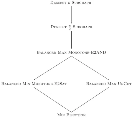
We summarise our inapproximability results by the following chains of reductions (Figure 1).
Densest k Subgraph
Densest n
2 Subgraph
Balanced Max Monotone-E2AND
Balanced Min Monotone-E2Sat Balanced Max UnCut
Min Bisection
Figure 1: Chains of E-reductions (bold line denotes an E-equivalence)
8
Dense Instances
In the previous chains of E-reductions the everywhere density is preserved except for the first reduction. Thus, since Min Bisection has a polynomial time approximation scheme on ev-erywhere instances [AKK95], all the above problems have a polynomial time approximation scheme on everywhere dense instances. Observe that the maximization problems Densest k Subgraph with k = Θ(n), Balanced Max Monotone-E2AND and Balanced Max Uncut have a polynomial time approximation scheme even for average dense instances, while Balanced Min Monotone-E2Sat and Min Bisection have no polynomial time approx-imation scheme for average dense instances [AKK95, BFK03].
9
Further Research
The results of our paper shed some light on the global classes of optimization problems con-nected to the constraint satisfaction problems. There are still several problems which are open. Can some of our inapproximability bounds be dramatically improved ?
Another important question is to find an alternative (to Khot’s technique [Kho04]) method of proving hardness results on some level of our chains in Section 7. Perhaps some "pure"
and explicit reduction methods can be developed for that. Another intriguing question is to construct approximation algorithms for global optimization problems studied in our paper with more satisfactory approximation factors than the best known up to now.
References
[AKK95] S. Arora, D. Karger and M. Karpinski, Polynomial time approximation schemes
for dense instances of NP-hard problems, Proceedings of 27th Annual ACM Sym-posium on the Theory of Computing, 1995, 284–293; also published in Journal of Computer and System Sciences 58, 1999, 193–210.
[ARV04] S. Arora, S. Rao and U. Vazirani, Expander flows and a √log n-approximation
to sparsest cut, Proceedings of the 36th Annual ACM Symposium on Theory of Computing (STOC 2004), 222 – 231.
[ACG+99] G. Ausiello, P. Crescenzi, G. Gambosi, V. Kann, A. Marchetti-Spaccamela, and M. Protasi, Complexity and approximation. Combinatorial optimization problems and their approximability properties, Springer, 1999.
[BFK03] C. Bazgan, W. Fernandez de la Vega and M. Karpinski, Polynomial time
approxi-mation schemes for dense instances of the minimum constraint satisfaction, Ran-dom Structures and Algorithms, 23(1), 2003, 73–91.
[BM02] M. Blaser and B. Manthey, Improved Approximation Algorithms for Max 2Sat with
Cardinality Constraint, The 13th Annual International Symposium on Algorithms and Computation (ISAAC 2002), LNCS 2518, 2002, 187–198.
[Cre95] N. Creigou, A dichotomy theorem for maximum generalized satisfiability problems, Journal of Computer and System Sciences, 51(3), 1995, 511–522.
[CKS01] N. Creignou, S. Khanna and M. Sudan, Complexity Classifications of Boolean Con-straint Satisfaction Problems, SIAM Monographs on Discrete Mathematics and Applications, 2001.
[CP91] P. Crescenzi and A. Panconesi, Completeness in approximation classes,
Informa-tion and ComputaInforma-tion, 93, 1991, 241–262.
[DMS99] I. Dumer, D. Micciancio and M. Sudan, Hardness of Approximating the Minimum
Distance of a Linear Code, Proceedings of the 40th Annual Symposium on Foun-dations of Computer Science, 1999, 475–484.
[Fei02] U. Feige, Relations between average case complexity and approximation complexity, Proceedings of the 34th Annual ACM Symposium on Theory of Computing (STOC 2002), 534–543.
[FK00] U. Feige and R. Krauthgamer, A polylogarithmic approximation of the Minimum
Bisection, Proceedings of the 41st Annual Symposium on Foundations of Computer Science, 2000, 105–115.
[FL01] U. Feige and M. Langberg, Approximation Algorithms for Maximization Problems
[GJ76] M. R. Garey and D. S. Johnson, Computers and intractability. A guide to the theory of NP-completeness, Freeman, C.A. San Francisco (1979).
[GVY93] N. Garg, V. Vazirani and M. Yannakakis, Approximate max-flow min-(multi)cut
theorems and their applications, Proceedings of the 25th Annual ACM Symposium on Theory of Computing (STOC 1993), 698–707.
[HZ01] E. Halperin, U. Zwick, A unified framework for obtaining improved approximation algorithms for maximum graph bisection problems, Proceedings of the 8th Con-ference on Integer Programming and Combinatorial Optimization (IPCO 2001), 210–225.
[Has97] J. Håstad, Some optimal inapproximability results, Proceedings of the 29th Annual ACM Symposium on Theory of Computing (STOC 1997), 1-10.
[Hof03] T. Hofmeister, An Approximation Algorithm for Max 2Sat with Cardinality
Con-straint, Proceedings of the 11th Annual European Symposium on Algorithms, 301– 312, 2003.
[Hol02] J. Holmerin, PCP with Global Constraints – Balanced Homogeneous Linear
Equa-tions, Manuscript, 2002.
[HK03] J. Holmerin and S. Khot, A strong inapproximability result for a generalization of Minimum Bisection, Proceedings of the 18th IEEE Conference on Computational Complexity, 371–378, 2003.
[HK04] J. Holmerin and S. Khot, A new PCP Outer Verifier with Applications to
Homoge-neous Linear Equations and Max-Bisection, Proceedings of the 36th Annual ACM Symposium on Theory of Computing (STOC 2004), 11–17.
[JS04] G. Jäger, A. Srivastav, Improved Approximation Algorithms for Maximum Graph
Partitioning Problems, Proceedings of the 24th International Conference Founda-tions of Software Technology and Theoretical Computer Science (FSTTCS 2004), 348–359.
[KMSV94] S. Khanna, R. Motwani, M. Sudan and U. Vazirani, On syntactic versus compu-tational views of approximability, Proceedings of the 35th Annual IEEE Annual Symposium on Foundations of Computer Science, 819–830, 1994, Also published in SIAM Journal on Computing, 28(1), 1999, 164–191.
[KS96] S. Khanna and M. Sudan, The optimization complexity of constraint satisfaction
problems, Technical note STAN-CS-TN-96-29, Stanford University, CA, 1996. [KST97] S. Khanna, M. Sudan and L. Trevisan, Constraint Satisfaction: the Approximability
of Minimization Problems, Proceedings of 12th IEEE Computational Complexity, 1997, 282–296.
[KSTW01] S. Khanna, M. Sudan, L. Trevisan and D. P. Williamson, The Approximability of Constraint Satisfaction Problems, SIAM Journal of Computing, 30(6), 1863-1920 (2001).
[KSW97] S. Khanna, M. Sudan and D. Williamson, A Complete Classification of the Approx-imability of Maximization Problems Derived from Boolean Constraint Satisfaction, Proceedings of 29th ACM Symposium on Theory of Computing (STOC 1997), 11–20.
[Kho04] S. Khot, Ruling Out PTAS for Graph Min-Bisection, Densest Subgraph and
Bipar-tite Clique, Proceedings of the 45th Annual IEEE Annual Symposium on Founda-tions of Computer Science (FOCS 2004), 136–145.
[PY91] C. H. Papadimitriou and M. Yannakakis, Optimization, approximation, and
com-plexity classes, Journal of Computing and System Science, 43 (1991), 425-440. [Sch78] T. Schaefer, The complexity of satisfiability problems, In Conference Record of the
10th Annual ACM Symposium on Theory and Computing (STOC 1978), 216–226. [Svi01] M. I. Sviridenko, Best possible approximation algorithm for MAX SAT with