Nonfattening condition for the generalized evolution by mean curvature and applications
16
0
0
Texte intégral
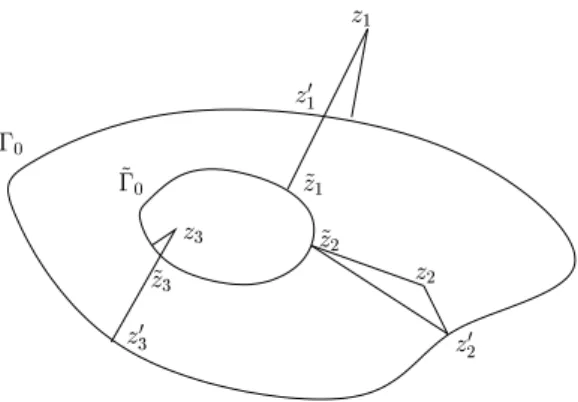
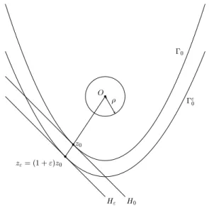
Figure
Documents relatifs
