Commodity Currencies Revisited
Evgenia Passari
Université Paris Dauphine
Current Draft: January 2015
Abstract
I build an exchange rate strategy that trades currencies conditional on changes in the global prices of commodity indices; hence, termed “commodity strategy”. First, I document that commodity prices have signi…cant out-of-sample forecasting ability for the future exchange rates of several commodity exporters and importers at the daily frequency. However, I report that the reverse forecasting relationship does not survive out-of-sample testing. Second, I …nd a signi…cant cross-sectional spread, in both spot and excess returns, of 6% p.a. between the currencies that are predicted to appreciate and those that are predicted to depreciate. The returns appear to be uncorrelated to those of popular exchange rate strategies such as the carry trade and currency momentum. Furthermore, the spread in returns is not explained by traditional risk factors; however, it is partly accounted for by the strategy’s high transaction costs. Net pro…tability can be restored by either implementing a simple market timing rule or by investing in developed markets with low costs and high liquidity.
Keywords: Foreign Exchange; Commodity Currencies; Asset Pricing. JEL Classi…cation: F31; F37; G10; G11.
Acknowledgements: The author is indebted for useful conversations and constructive comments to Lucio Sarno. I also thank Ian Marsh, Richard Payne, Hélène Rey, Elias Papaioannou, my colleagues at Cass Business School and London Business School and the participants of the 12th Conference on Research on Economic Theory and Econometrics as well as the participants of the 2013 European Summer Symposium in Financial Markets. I am especially grateful to Cheng Yan, Vania S tavrakeva, Robert Ready, Francisco Gomes, Ralph Koijen, Hanno Lustig, Timothy Mcquade, S tefan Lewellen, Kleopatra Nikolaou and Deepa Dhume Datta. The usual d isclaimer applies. Corresponding author : Evgenia Passari, Université Paris Dauphine, Place du Maréchal de Lattre de Tassigny, 75016 Paris, France. E-mail: e [email protected].
1
Introduction
Commodity prices and exchange rates are linked in fundamental ways1. However, little is known about how this relationship evolves in the cross-section2. In this paper, I show that commodity
prices contain signi…cant information about the cross-section of future currency returns. I begin by showing that daily changes in commodity price indices can be used to forecast day-ahead movements in exchange rates. I then construct a trading strategy that takes a long (short) position in currencies that are expected to appreciate (depreciate), based on prior day’s commodity price movements. I …nd that the returns on this long-short portfolio are approximately 6 per cent per annum. Portfolio returns peak in the heart of the recent …nancial crisis. They also appear to be uncorrelated with returns on other popular strategies such as the carry trade and currency momentum. Unlike existing studies of the commodity-currency relationship3, I report out-of-sample (OOS) forecasting ability
for the exchange rate using information from lagged commodity returns; on the contrary, the reverse forecasting regression does not survive OOS testing – that is, exchange rates do not forecast future commodity prices. Furthermore, the forecasting relationship between commodity price movements and currency returns weakens signi…cantly as the forecasting period is lengthened from the daily level to the weekly and monthly levels. Together, these results suggest that although the information in commodity price movements is not re‡ected in exchange rates instantaneously, it does eventually get incorporated into currency prices after some time.
In recent years, commodity prices have reached all-time highs which have been followed by signif-icant drops, the most notable one occurring towards the end of 2008. The increase in the popularity of commodity investing during the past decade has also been remarkable, rendering the study of the interrelation between commodities and other asset markets an important endeavour. The theoreti-cal relationship between commodity prices and currencies relies on simple intuition: for commodity exporters, ‡uctuations in world commodity prices explain a large share of movements in their terms of trade (Bidarkota and Crucini (2000)). This is, in turn, a key determinant to exchange rate ‡uctuations (De Gregorio and Wolf (1994), Chinn and Johnston (1996), Montiel (1997). Recently, Ready, Roussanov and Ward (2013), provide a new theory for the relationship between exchange
1Research work by Chen and Rogo¤ (2003), Cashin Cespedes and Sahay (2004), and Chen, Rogo¤ and Rossi (2010),
among others, link changes in world commodity prices with national real exchange rates of commodity exporting countries (commodity currencies), through the terms of trade channel and establish a long-run relationship between the two variables.
2There is a growing literature that deals with the cross-section of currency returns following the landmark work of
Lustig and Verdelhan (2007). See also Lustig, Roussanov, and Verdelhan (2011) and Menkho¤, Sarno, Schmeling and Schrimpf (2012a) among other studies.
3
Chen, Rogo¤ and Rossi (2010) argue that “commodity currency exchange rates have remarkably robust power in predicting global commodity prices, both in-sample and out-of-sample, and against a variety of alternative benchmarks”. The authors maintain that the reverse relationship is signi…cantly less powerful. Clements and Fry (2006) report similar results.
rates and commodities, and report that a commodity-based strategy explains a substantial portion of the carry-trade risk premia, and all of their pro-cyclical predictability with commodity prices and shipping costs. Overall, the literature studying the relationship between exchange rates and commodity prices documents the existence of an empirical link, but the direction of predictability remains largely unclear.
One of the key contributions of the present paper is the study of the economic structure of “commodity forecasted” returns in FX markets by gathering information from a large cross section of exchange rates. The evidence on the predictive ability of commodities in the cross-section of currencies is very limited as the literature has generally focused on time-series studies. In this context, it is natural to employ the portfolio approach given its emerging popularity and success in the study of currency behaviour. In my empirical analysis, I follow the recent literature (Lustig and Verdelhan (2007), Lustig, Roussanov, and Verdelhan (2011)) and Menkho¤, Sarno, Schmeling and Schrimpf (2012a)), and sort currencies into portfolios according to the predictions of the proposed commodity strategy. I start by forming currency portfolios where an investor is long in currencies with the highest predicted returns and short in currencies with the lowest predicted returns. I take the view of a U.S. investor and employ exchange rates against the U.S. dollar (USD). The data cover the period between January 2000 and November 2011, and I study a cross-section of 25 currencies. Throughout the empirical exercise I employ tradable commodity price indices in order to circumvent potential liquidity issues4. Then, as in Lustig, Roussanov, and Verdelhan (2011), I cross-sectionally
relate the returns of the commodity strategy to a set of risk factors.
I employ daily, weekly and monthly data, as unlike most fundamental variables, commodity prices allow the possibility of …ner sampling. Higher frequency data present the advantage of resolving empirical pitfalls such as temporal aggregation5. The motivation to look at the daily horizon is also driven by the empirical …nding that short-term predictability has been extremely elusive throughout the exchange rate literature. Apart from the studies of currency order ‡ow, a high frequency, almost contemporaneous, relationship between the exchange rates and fundamentals has only been reported by the literature of macroeconomic news announcements (Andersen, Bollerslev, Diebold and Vega (2003) and Faust, Rogers, Wang and Wright (2007). The recent work of Ferraro, Rogo¤ and Rossi (2012) is probably the …rst to document out-of-sample exchange rate predictability in the short run, using fundamental information (oil prices) that arrives at high frequency. Nevertheless, their analysis is primarily focused on the forecasting ability of oil prices, for the Canadian dollar. On the other
4
These indices provide a benchmark for investment in the commodity markets while serving as a measure of com-modity performance over time. They are available to market participants of the Chicago Mercantile Exchange.
5
As Alan Taylor (2001) observes, “if we suspect that the actual adjustment horizon is of the order of days, then monthly and annual data cannot be expected to reveal it ”.
hand, their results regarding a handful of commodity currencies paint a mixed picture when it comes to out-of sample forecasting.
In line with the literature on commodity currencies, I document a strong relationship between commodities and exchange rates; I …nd that commodity prices have signi…cant out-of-sample (OOS) predictive ability for the future exchange rates for 16 out of 25 commodity exporters and importers, on the daily frequency. The OOS predictive ability of lagged commodity prices for the exchange rate weakens when moving from the daily to the weekly frequency and almost disappears in the monthly frequency, which is consistent with the temporal aggregation argument. Commodity prices also Granger-cause exchange rates in 20 out of 44 cases on the daily frequency, but the relationship becomes weaker on weekly and monthly frequencies. However, unlike the …ndings of Chen, Rogo¤ and Rossi (2010), I report that the reverse forecasting regression provides weaker Granger-causality evidence in all cases and does not survive out-of-sample testing. This result is mainly attributed to the larger country sample under examination. I report that the proposed “commodity strategy”, when implemented daily, leads to economically signi…cant, unconditional spot excess returns that appear uncorrelated to popular FX strategies such as the carry trade and currency momentum. In addition, a sub-sample exercise reveals that the strategy works well across the sample period but displays even stronger performance during the crisis period.
Currency markets are among the most liquid in the world, displaying large transaction volumes and low transaction costs, while their participants are to a large extent professional investors, facing no short-selling constraints. Hence, if markets are e¢ cient, any information that is contained in com-modity price movements should be re‡ected in exchange rates instantaneously. In order to account for these high returns, I explore whether the “commodity strategy” is a¤ected by (i) measures of risk that have been found to fare well in the exchange rate literature, such as global FX volatility risk and currency momentum (e.g. see Menkho¤, Sarno, Schmeling and Schrimpf (2012a and b)), (ii) risk factors motivated by the equity market literature and (iii) transaction costs. I …nd that the returns cannot be explained in a linear asset pricing framework (Ang, Hodrick, Xing, and Zhang (2006)) by standard measures of exchange rate risk; nevertheless, factors such as the interest rate and the equity market appear to negatively correlate with the strategy returns. However, the im-pact of transaction costs is non-trivial; adjusting returns for bid-ask spreads can erode pro…tability completely. This is particularly true when the strategy is implemented using a number of emerging market currencies which display large bid-ask spreads which act as barriers to arbitrage activity. The exploitability problem can, however, be circumvented if the investor trades only developed market currencies, which showcases the validity of the strategy for di¤erent exchange rate panels. In essence, the ordered portfolios need not necessarily be skewed towards currencies with high transaction costs.
I also investigate the performance of a simple market timing strategy. I next turn to mispricing: when there is slow information di¤usion / limited attention, it takes time for information to be transmitted from one asset class to another (Daniel, Hirshleifer, and Teoh (2002), Hirshleifer and Teoh (2003) and Lim and Teoh (2010)). Since prices should eventually re‡ect information, return predictability should fade away with the passage of time. My …ndings suggest that this is indeed the case; return predictability using lagged commodity prices holds at the daily level, but weakens signi…cantly at the weekly and monthly level.
My work also contributes to the literature that investigates the relationship between exchange rates and fundamentals. The link between exchange rates and economic fundamentals has been elusive, especially for short horizons, and various anomalies have emerged throughout the years6.
Commodity currencies have been known to o¤er an attractive laboratory for the study of this link7. The relationship between currencies and commodities was …rst observed by Amano and Norden (1993) and Gruen and Kortian (1996). Despite the likely omission of other explanatory variables, a simple, empirical model of commodity prices and exchange rates has shed some light on the relationship between commodities and expected exchange rate returns. Chen and Rogo¤ (2003) document that the US dollar price of commodity exports has a signi…cant e¤ect on the real exchange rates of Australia, New Zealand, and to a lesser extent, Canada. Follow-up work by Cashin, Cespedes and Sahay (2004), among others, provides evidence of a long run relationship between real exchange rates and real commodity prices for approximately one third of the commodity-exporting countries in their sample. An important strand of this literature has also focused on the forecasting power of commodities for the exchange rate, reporting limited predictability success, except for the recent work of Ferraro, Rogo¤ and Rossi (2012), who …nd robust evidence at the daily frequency. At the same time, currencies are found to forecast commodity price changes with relative success. Clements and Fry (2006) …nd less evidence that currencies are a¤ected by commodities than that commodities are a¤ected by the commodity currencies. In the same lines, Chen, Rogo¤ and Rossi (2010) argue that “commodity currency exchange rates have remarkably robust power in predicting global commodity prices, both in-sample and out-of-sample, and against a variety of alternative benchmarks”, although the reverse relationship is found to be signi…cantly less powerful. Their theoretical explanation is that exchange rates are forward looking, while commodity price ‡uctuations are more prone to short-term demand imbalances.
6
The puzzles in exchange rate economics relate to the most prominent fundamental models, namely the Uncovered Interest rate Parity (UIP), Purchasing Power Parity (PPP) and Monetary Fundamentals model (MF), and have been extensively studied by …nance scholars (Obstfeld and Rogo¤ (2000)).
7
As Chen, Rogo¤ and Rossi (2010) observe, a simple model of exchange rates and commodities is less impaired by endogeneity issues as compared to other exchange rate models that employ standard macroeconomic fundamentals.
Overall, a careful reading of the literature on commodity currencies suggests that commodity prices emerge as a variable of signi…cance for the exchange rate. Along these lines, there could exist a positive or negative price of commodity risk. I deviate from the traditional approach motivated by the observation that, so far, it has yet to be established whether a currency investor could bene…t from the information embedded in commodity price changes extracting information from the section of returns. I go beyond earlier work on commodity currencies by exploring the cross-sectional dimension in an asset pricing framework and by extending the country panel to include both commodity exporters as well as importers in order to study whether the documented relationship holds for commodity currencies only,
The remainder of the paper is organized as follows. Section 2 sets the framework employed in the construction of the proposed commodity strategy. Section 3 describes the data and presents the results of the Granger-causality tests and the out-of-sample forecasting exercise. Section 4 presents descriptive statistics for the formed currency portfolios and compares the commodity strategy to the carry trade. Section 5 presents the results from the asset pricing exercise. Section 6 discusses the potential importance of other factors such as the interest rate and the equity market. In Section 7, I report the robustness checks and presents a simple market-timing exercise. Section 8 concludes.
2
Framework for the Commodity Strategy
As primary commodities dominate the exports of several countries, ‡uctuations in world commod-ity prices potentially explain a non-trivial share of movements in their terms of trade (Bidarkota and Crucini (2000)). At the same time, terms of trade ‡uctuations have long been considered a key determinant of real exchange rates (De Gregorio and Wolf (1994), Chinn and Johnston (1996), Montiel (1997)). Research work by Chen and Rogo¤ (2003) and Cashin Cespedes and Sahay (2004) link changes in world commodity prices with national real exchange rates of commodity exporting countries through the terms of trade channel and establish a long-run relationship between the two variables. The intuition is simple: for commodity exporters, whose size in the world commodity market is relatively small to justify the assumption that they are a price-taker in that market, ‡uc-tuations in world commodity price movements generally explain a large share of movements in their terms of trade, which in turn is a key determinant to the exchange rate ‡uctuations8. As
improve-8Ready, Roussanov and Ward (2013), using a model of the shipping industry to model trade costs, provide a new
theory for the relationship between exchange rates and commodities, and report that a commodity-based strategy explains a substantial portion of the carry-trade risk premia, and all of their pro-cyclical predictability with commodity prices and shipping costs. They show that the di¤erences in average interest rates and risk exposures between countries that are net importers of basic commodities and commodity-exporting countries can be explained by appealing to a natural economic mechanism, trade costs. However, their empirical strategy is static; hence, their results are of di¤erent nature than those of the present study.
ment in the terms of trade through an increase of export prices will lead to currency appreciation, deterioration in the terms of trade through an increase of import prices will cause depreciation of the currency. Following this line of reasoning, I argue that commodity price movements are of great importance to commodity importers as well.
Figure 1, shows that the link between commodity prices and the terms of trade of commodity exporters is tight. Speci…cally, the terms of trade of Canada display an evident comovement with the price of brent and natural gas; the same is true for the terms of trade of Mexico and the price of brent and silver and for the terms of trade of Brazil and the price of brent and agriculturals. What is of particular interest is the evolution of the terms of trade of Japan, a major commodity importer, with the price of brent.
FIGURE 1 ABOUT HERE
Japan’s terms of trade are worsening with the rise of brent price and vice versa. Naturally, the exchange rate of big “net importers” is also prone to commodity price shocks through the terms of trade channel. It follows that one can study the link between exchange rates and commodity prices by exploiting information from a larger cross-section of countries irrespective of their trade balance.
Since the scope of my analysis is to compile a country panel that consists both of commodity importers and exporters, it is important to be accurate about the commodities that could have an actual impact on the exchange rate of each country. The estimation equation is based on a standard model of commodity prices and exchange rates, with the di¤erence that I allow the regressions to be country-speci…c, according to the most “important”commodity imports or exports for each country. I therefore distinguish among 25 di¤erent speci…cations of the basic regression equation by including on the RHS of the equation the commodities that account for …ve per cent - or above - of the total gross domestic product (GDP) of each country, according to data collected from the United Nations Commodity Trade Statistics Database, for which there exist tradable commodity index series (see Table 1.):
sk;t+1= ak+
X
m2M
k;m Pt;m+ uk;t+1; (1)
where st+1 st+1 st, st denotes the logarithm of the spot exchange rate (foreign price of
domestic currency, with US dollar being the domestic currency) at time t, k stands for the country, Pt is the commodity price change, m denotes a commodity that constitutes …ve per cent or more
of the country’s GDP, M is the total of all commodities that are important for each country, and ut+1 is the forecast error. By including commodities individually, instead of constructing an index, I
allow the exchange rate to respond di¤erently to individual commodity price changes. Furthermore, Bidarkota and Crucini (2000), …nd that variation in the world prices of three or fewer key exported commodities account for 50% or more of the annual variation in a country’s terms of trade.
TABLE 1 ABOUT HERE
Table 1 also reports the betas of the full sample estimation of equation (1) along with their statistical signi…cance. An increase in the price of commodity exports always coincides with an appreciation of the foreign currency and this is a statistically signi…cant result. However, a price increase of commodity imports - an increase in the price of brent for a net brent importer for instance - does not necessarily correspond to foreign currency depreciation; the USA being the biggest brent importer bares a heavier burden of the crude price increases through a relatively bigger deterioration of their terms of trade, leading most of the times to an appreciation of the foreign currency (all exchange rates are quoted versus the US dollar). However, the coe¢ cient for Japan (another large brent importer) is negative, suggesting that a rise in the price of crude coincides with a depreciation of the Japanese yen the following period.
As an additional preliminary check, the currencies are ranked in terms of their betas from an estimated regression of the currencies on the composite Spot Commodity Index from the Standard & Poors, Goldman Sachs Commodity Index spot price series (formerly the Goldman Sachs Commodity Index series)9, by using both the US dollar and the British pound as a numeraire. This constitutes the only non-country speci…c estimation and it is employed for purely illustrative purposes. The rankings are displayed in Table 2. In both cases, the commodity currencies populate the top of the table, corresponding to betas which are higher in value, providing a …rst indication that the estimated relationship between currencies and commodities yields meaningful estimates. In other words, commodity currencies respond on average “more aggressively” to commodity price changes.
TABLE 2 ABOUT HERE
3
Data and Empirical Analysis
The present section details the currency and price data used in the empirical exercise. The data for spot exchange rates and 1-month forward exchange rates versus the US dollar (USD) and the British
9
pound (GBP) (via triangular arbitrage) cover the sample period from January 2000 to November 2011, and are obtained from Reuters (via Datastream). The reason I choose to restrict my sample to the past decade is that I wish to restrict the periods of in‡ation and exchange rate turmoil, relevant for some of the countries in my sample prior to 2000. The empirical analysis is carried out at the daily, weekly, and monthly frequency and I work in logarithms of spot and forward exchange rates. My panel comprises the following 25 countries: Australia, Brazil, Bulgaria, Canada, Chile, Croatia, Czech Republic, Euro area, Hungary, India, Indonesia, Israel, Japan, Mexico, New Zealand, Norway, Philippines, Poland, Russia, Singapore, South Africa, Sweden, Switzerland, Thailand and the United Kingdom.
With respect to the commodity price series, I employ the Standard & Poors, Goldman Sachs Commodity Index spot price series (formerly the Goldman Sachs Commodity Index series) which serve as a benchmark for investment in the commodity markets, for the following commodities: agriculturals, aluminium, brent crude, copper, energy, gold, industrial metals, livestock, natural gas, precious metals, silver and wheat. I construct the commodity shares using data from the United Nations Commodity Trade Statistics Database.
3.1 Granger-Causality Tests and Out-of-Sample Forecasts
In the present section, I examine the in-sample and out-of-sample forecasting ability of commodity prices for the exchange rate and vice versa, following the …ndings of Chen, Rogo¤ and Rossi (2010). For this purpose, I look at the relationship between exchange rates and commodity prices both in terms of Granger-causality and out-of-sample forecasting ability relative to the random walk (RW), given its prevalence as a benchmark in the exchange rate literature.
3.1.1 Do Commodity Prices Contain Information about Exchange Rates?
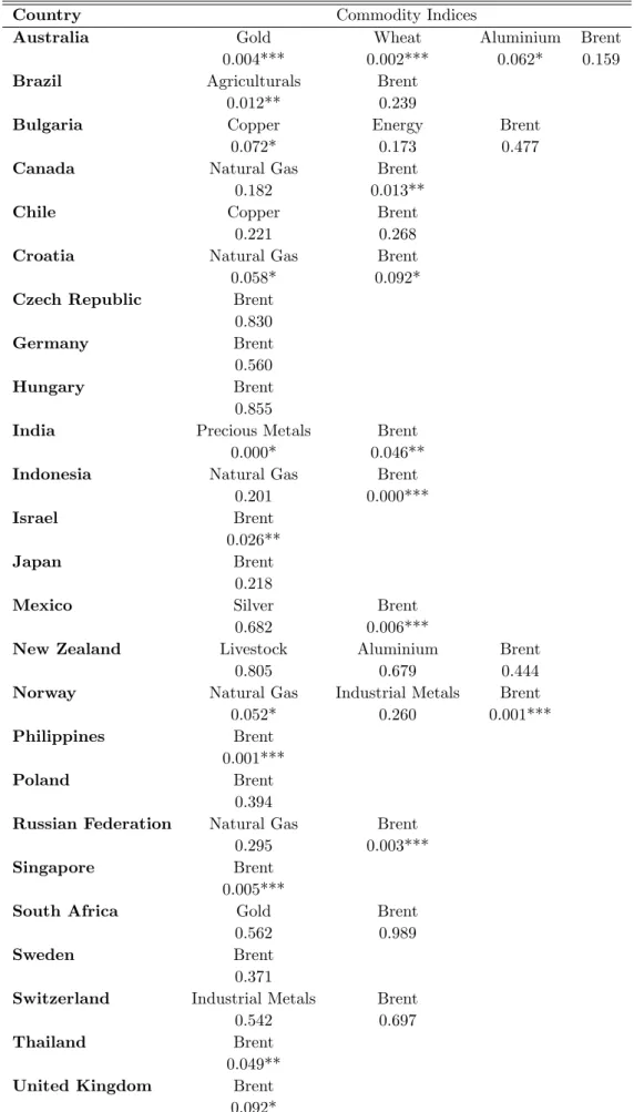
I …rst study the empirical evidence on in-sample Granger-causality, following the traditional testing procedure. The analysis includes one lag of each of the explanatory and dependent variables, but the overall picture is not altered with the inclusion of additional lags. Table 3 reports the results, for the daily frequency, based on a standard Granger-causality regression of the type:
st+1= 0+ 1Pt+ 2 st+ ut+1
for the 25 exchange rates and their corresponding commodity price indices. The table reports the p-values for the test of the null hypothesis that 0 = 1 = 0 , so a number below 0.05, for instance,
implies evidence in favor of Granger-causality (at the 5 per cent level). In general, Granger-causality tests …nd some evidence of commodity prices Granger-causing exchange rates as the null of no Granger-causality is rejected for 20 out of the 44 cases. The results for the weekly and monthly frequency are reported in Tables 1 and 2 of the Appendix. In general, the results appear weaker in lower frequencies. In particular, commodity prices are found to Granger-cause exchange rates only 21% percent of the times on the weekly frequency and 14% of the times on the monthly frequency. What is striking though, is that commodity importers constitute a non-trivial part of the subsample of the countries for which IS predictability is detected. This is a robust …nding across frequencies.
TABLE 3 ABOUT HERE
I complement this part of the analysis with an out-of-sample forecasting exercise. In particular, I estimate the country-speci…c regressions using a rolling window of three years. As Chen, Rogo¤ and Rossi (2010) note, one should keep in mind that many commodity exporters experienced major changes in policy regimes and / or market conditions. Hence, the importance of allowing for time-varying parameters should not be undermined. For this purpose, I estimate each model using the …rst 780 data points (three years of data) for the initial one-period-ahead forecast to be generated. Subsequently, the …rst data point is discarded while an additional data point at the end of the sample is added and the model is re-estimated. For each of the models described above I construct a one-day-ahead forecast at each step. The data from January 2000 to December 2002 are employed for estimation and the rest are saved for out-of-sample forecasting. The out of sample forecasts, hence, refer to the period between January 2003 and November 2011.
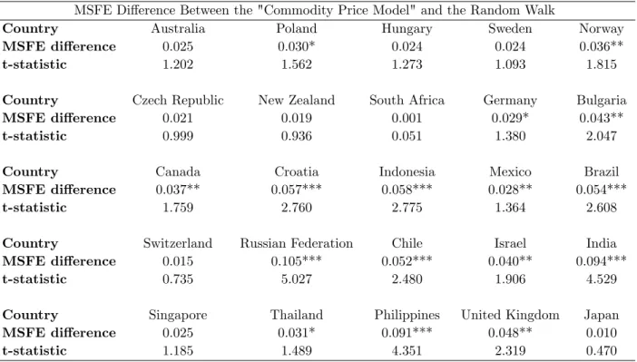
I report results relative to the random walk benchmark due to its signi…cance in the exchange rate literature. I report the di¤erence between the mean square forecast error (MSFE) of the “commodity price model” and the MSFE of the RW benchmark, re-scaled by their variability. I further present the t-statistics of the test of equal forecasting performance (Clark and West, 2006) to compare the two nested models. A t-statistic greater than +1.282 (for a one-sided 0.10 test) or +1.645 (for a one-sided 0.05 test) implies that the larger model contains out-of-sample forecasting power for the dependent variable.
Table 4 shows that commodity prices have some forecasting ability for exchange rates, even out-of-sample on the daily frequency. The “commodity price model”outperforms the RW benchmark in forecasting exchange rate changes for 16 out of 25 countries. This number falls to 8 for the weekly frequency and to 3 for the monthly frequency (Appendix tables 3 and 4).
Overall, the evidence in favour of in-sample predictability and OOS forecasting power of com-modity prices for the exchange rate, at daily frequency, is quite striking. The …ndings however are not robust moving to weekly and monthly lower frequencies suggesting ephemeral predictability, in line with the results of Chen, Rogo¤ and Rossi (2012). However, it appears that the daily forecasting power of commodity prices for the exchange rate is a general result which is not unique to oil prices and / or commodity exporters.
TABLE 4 ABOUT HERE
3.1.2 Do Exchange Rates Contain Information about Commodity Prices?
I repeat the Granger-causality test and the out-of-sample exercise in order to test for the reverse relationship, i.e. if exchange rates contain information about commodity prices.
The Granger-causality regression is now of the type:
Pt+1 = 0+ 1 st+ 2 Pt+ ut+1
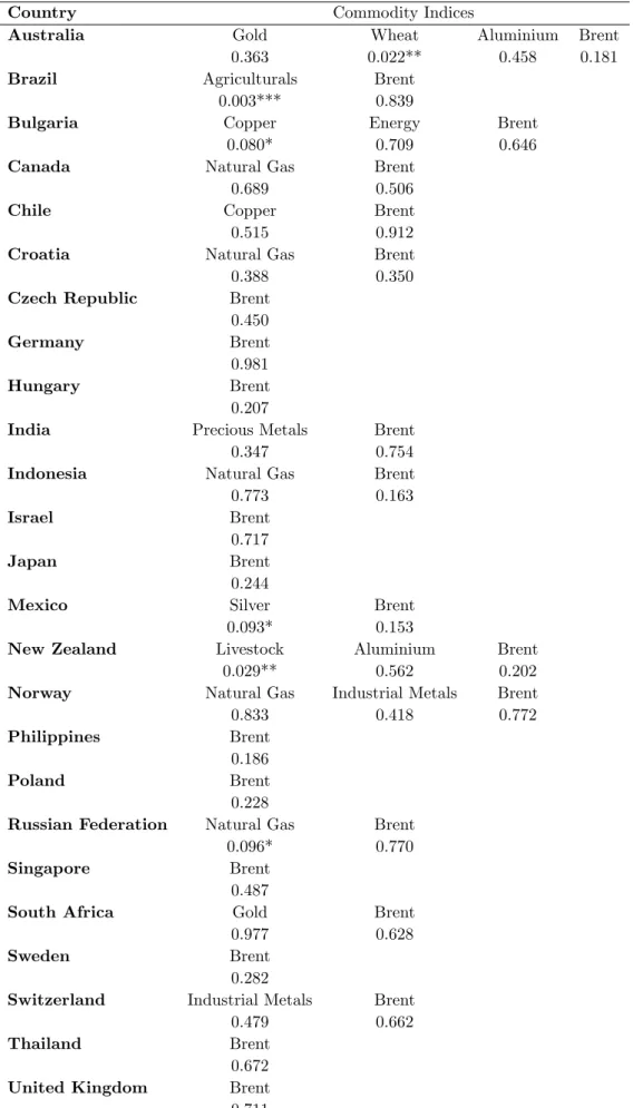
Again, Table 5 reports the results of the p-values for the test of the null hypothesis that 0 =
1 = 0. In this instance, causality tests report little evidence of exchange rates
Granger-causing commodity prices as the the null of no Granger-causality is rejected only for six out of the 44 cases.
TABLE 5 ABOUT HERE
In addition, the out-of-sample analysis shows little evidence of exchange rate changes forecasting commodity price changes better than the RW benchmark. Table 6 shows that exchange rates have little forecasting ability for brent prices out-of-sample. The “exchange rate model” outperforms the RW benchmark in forecasting brent price changes for only 3 out of 25 countries. The predictive ability of the exchange rate for other commodity prices -not reported here to conserve space but available upon request - paints a similar picture.
TABLE 6 ABOUT HERE
Both exercises are repeated in weekly and monthly frequencies. The results appear robust across frequencies and are reported in Tables 5 through 8 of the Appendix.
3.2 Commodity Portfolios and Descriptive Statistics
The present section moves beyond statistical predictability. Given the long-established relationship between commodities and currencies and the encouraging results of the previous section on the daily frequency, a natural step is to investigate the economic structure of “commodity forecasted”returns in FX markets, gathering information from the cross section of currency returns. Remarkably, the evidence on the predictive ability of commodities in the cross-section of currencies is very limited, as the literature has generally focused on time-series studies.
Following Lustig and Verdelhan (2007), I sort currencies according to the forecasted returns of the commodity strategy and allocate them to portfolios. Unlike their work, I focus on daily investment horizons and perform the exercise using both spot and excess returns. In both cases, Portfolio 1 contains the currencies with the highest sell signal and Portfolio 5 contains the currencies with the highest buy signal. I further construct an Average Portfolio that contains all the currencies and a Corner Portfolio which essentially invests in the long-short strategy: Portfolio 5 - Portfolio 1. A typical example is the following. Let us consider a US investor who builds a portfolio by allocating her wealth among 25 assets that are identical in all respects except for the currency of denomination (GBP, CHF, JPY, CAD, AUD, NZD, SEK, NOK, EUR, ZAR, SGD, CZN, HUF, INR, IDR, MXN, PHP, THB, PLN, BRL, RUB, HRK, ILS, BGN, and CLP). The main objective of the analysis is, to determine whether there is economic value in predicting the FX returns using commodity price changes as a criterion for portfolio selection. The investor rebalances her portfolio on a daily basis by taking a long position on the …ve currencies that she expects to appreciate the most, simultaneously shorting the …ve currencies that she projects to depreciate the most, over the horizon of one day. Each day she takes two steps. First, she uses the respective model to forecast the cumulative long-short portfolio return. Second, conditional on the forecast, she dynamically rebalances her portfolio following the long-short strategy described above. The return from domestic riskless investing is proxied by the 1-month US Eurodeposit rate. All portfolios are equally weighted and the excess returns for each one of them are calculated as follows:
rt= ln(St+1) ln(Ft) (2)
where Ft is the one-day forward exchange rate.
In order to measure the economic value of each strategy, I rely on the Sharpe Ratio, which is a commonly used measure of economic value in the context of mean-variance analysis. In assessing the
pro…tability of the dynamic strategies, at this stage, the e¤ect of transaction costs is not taken into consideration.
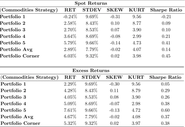
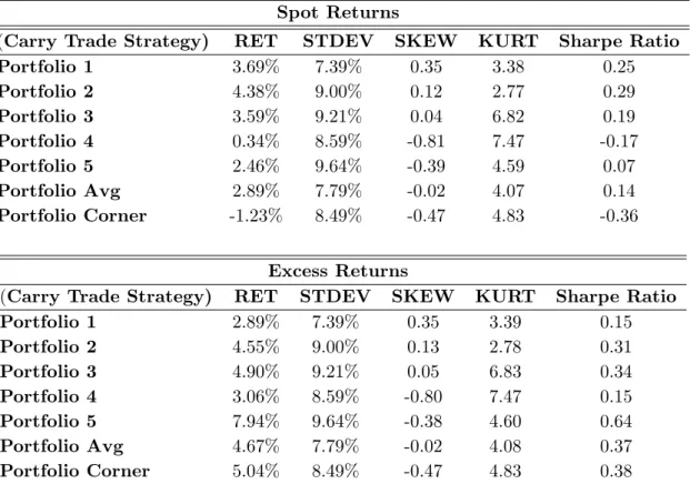
The descriptive statistics for the seven commodity portfolios are displayed in Table 7 for the spot ( st+1) and excess return (ln(St+1) ln(Ft)) cases. The results show that there appears to be
high economic value associated with the Corner Portfolio strategy. Additionally, the returns and the Sharpe Ratios of the strategies are monotonically increasing as one moves from Portfolio 1 to Portfolio 5, using either the spot or excess returns series. There is not a clear monotonic pattern regarding the standard deviations, and the skewness and kurtosis measures. However, one can observe that the extreme values with respect to the second, third and fourth moments consistently appear in Portfolios 1 and 5.
TABLE 7 ABOUT HERE
At this point one should note that the inspection of Table 7 reveals something more important. Although the Average Portfolio’s Spot Return is lower than the Average Portfolio’s Excess Return, (2.89% versus 4.67%), the Corner Portfolio’s Spot Return is greater than the Corner Portfolio’s Excess Return (6.03% versus 5.32%), which is in stark contrast to what the literature in carry trades tells us about the return nature of the carry strategy. This result o¤ers a clear, …rst indication that the returns to the commodity strategy are potentially uncorrelated with the returns to standard exchange rate strategies such as the carry trade. In order to test for this, as a …rst step, I construct …ve carry trade portfolios with the exchange rates sorted into portfolios according to their lagged forward premium, as in Lustig and Verdelhan (2007).
4
Comparing the Commodity Strategy to Carry Trade
It is of great importance to know whether the constructed commodity strategy does nothing more than simply replicating the nature of returns of other popular exchange rate strategies such as the carry trade. My …ndings point out that is not the case.
For this purpose, I build a standard carry trade strategy and repeat the portfolio formation process. The currencies are again allocated to …ve portfolios based on their forward discounts at the end of period t. Sorting on forward discounts is equivalent to sorting on interest rate di¤erentials since Covered Interest Parity holds closely in the data at the frequency analyzed in this paper (see e.g. Akram, Rime, and Sarno (2008)). I re-balance the portfolios at the end of each day. This is repeated day by day during the corresponding period. Currencies are ranked from low to high:
Portfolio 1 contains currencies with the lowest and portfolio 5 contains currencies with the highest interest rates. Daily excess returns for holding foreign currency k, say, are again computed as before.
The properties of carry trade-sorted portfolios are displayed in Table 8. The table presents descriptive statistics for the seven portfolios (as before, Portfolios 1-5, Average and Corner Portfolio) for both spot and excess returns.
TABLE 8 ABOUT HERE
The upper panel of Table 8 displays the results for the spot carry trade returns; a …rst observation is that there is not a monotonically increasing pattern in average returns. The Corner Portfolio ap-pears to be loss-making, yielding an annualized return of -1.23%. The higher moments of the return distribution also present a mixed picture with no pattern emerging. This does not necessarily con-stitute a puzzling …nding since the literature on carry trades focuses on the study of excess returns. Indeed, an inspection of the lower panel of Table 8, which presents the excess returns for the carry trade strategy, reveals that the returns and Sharpe Ratios of the carry trade and commodity corner portfolios are comparable. However, the higher moment patterns appear to be quite dissimilar. In particular, the carry trade strategy, when implemented on excess returns, displays almost monotoni-cally increasing annualized standard deviations moving from Portfolio 1 to 5. Skewness also displays a decreasing pattern.
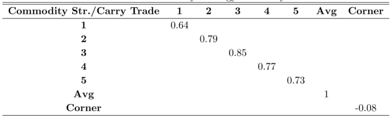
Furthermore, Table 9, presents the correlation coe¢ cients between the spot returns to the com-modity strategy and the spot returns to the carry trade strategy10. Correlations are reported between
corresponding portfolios. It is evident that despite the fact that correlations between the spot re-turns for Portfolios 1-5 are positive and quite substantial in magnitude, there is a marginally negative correlation of -0.084 between the returns of the two corner portfolios. Therefore, the returns to the two strategies are clearly uncorrelated; in fact, there should exist diversi…cation bene…ts when the commodity strategy is used in conjunction with the carry trade strategy.
TABLE 9 ABOUT HERE
Finally, following Menkho¤ et al. (2012b), I double-sort currencies into two portfolios depending on whether their lagged forward discount is above or below the panel median, and subsequently into two portfolios according to their forecasted value with respect to the commodity strategy regression.
1 0
Correlation coe¢ cients between the excess returns to the commodity strategy and the carry trade strategy are equal to the second decimal digit and are not, therefore, reported seperately.
The rebalancing frequency is always daily. The results of this exercise appear in Table 10. An inspection of the …ndings reveals that it makes a big di¤erence whether the commodity strategy is implemented in high or in low interest rate currencies. In particular, in the high interest rate currency environment, the strategy yields negative returns while in the low interest rate currency environment the revenues amount to a positive return of 4.42% per annum. Likewise, the carry trade appears to be pro…table only in the subsample of the currencies that are predicted to depreciate by the commodity strategy. In contrast, the carry trade is loss making in the subsample of the currencies that are predicted to appreciate by the commodity strategy.
TABLE 10 ABOUT HERE
Once again, the results do not indicate a positive relationship between the commodity strategy and the carry trade. However, it seems that one cannot easily achieve greater returns than those of the corner portfolios of the two strategies taken individually by following a double-sorting strategy which further reinforces the possibility of a hedging relationship between the two strategies.
As a natural step, in the following section I try to identify common factors in the cross-section of the commodity strategy’s currency returns (spot and excess).
5
Empirical Results
5.1 Common Factors in Currency Returns
Following Lustig, Roussanov and Verdelhan (2011) who employ a data-driven approach following the Arbitrage Pricing Theory of Ross (1976), I conduct a principal component analysis on Portfolios 1-5 of the commodity strategy. The results, portrayed in Table 11 (Panels I and II), show that the …rst two factors explain 87 per cent of the return variation of the commodity portfolios. The …rst 5 rows of the two panels reveal the factor loadings of the …ve commodity portfolios on principal components 1-5. The …rst principal component accounts for 75 per cent of the return variation. As in Lustig, Roussanov and Verdelhan (2011), who study the principal component analysis of the carry trade, the …rst principal component can be viewed as a level factor given that the loading of the portfolios always lies between 42 per cent and 47 per cent. The second principal component, accounts for 12 percent of the common variation. The loadings increase in a monotonic fashion across portfolios for the second principal component, which behaves in the same way as the "slope factor" of Lustig, Roussanov and Verdelhan (2011) and is hence, the sole candidate risk factor which can account for the cross-section of commodity portfolio returns. As in Lustig, Roussanov and Verdelhan (2011), I
employ the average currency return as my …rst factor, which I denote DOL. The correlation of the …rst principal component with DOL is found to be 0.99 which again constitutes a standard result.
TABLE 11 ABOUT HERE
5.2 Asset Pricing Methodology
This section brie‡y summarizes my approach to cross-sectional asset pricing. I rely on a standard SDF approach (Cochrane (2005)) as well as on a traditional Fama MacBeth two-pass OLS methodology (Fama and MacBeth (1973)) to estimate the factor risk prices and portfolio betas.
5.2.1 SDF Approach
The no-arbitrage relation holds so that risk-adjusted currency excess returns have a price of zero and satisfy the Euler equation:
E[mt+1rxit+1] = 0;
where mt= 1 b0(ht em), is the linear SDF , h stands for the risk factor vector, b is the SDF
parameter vector and em stands for the vector of factor means.
The setting suggests:
E[rxi] = 0 i;
a beta pricing model, in which expected excess returns depend on factor risk prices and risk quantities i for each portfolio i, where =Phb (Cochrane (2005)).
The Euler Equation is estimated using the generalized method of moments (GMM) of Hansen (1982). I do not use instruments apart from a constant vector of ones. The factor means em and the elements of the covariance matrix of h are estimated simultaneously with the SDF parameters via adding the respective moment conditions to the asset pricing moment conditions implied by the Euler equation. The one-step speci…cation allows one to su¢ ciently account for estimation uncertainty as Burnside (2009) notes.
Tables 14-15 present and estimates with Newey and West (1987) standard errors, cross-sectional R2s;and the Hansen-Jagannathan (HJ) distance metric (Hansen and Jagannathan (1997)) with simulated p-values.
5.2.2 Fama MacBeth Approach
I also employ the FMB two-pass OLS methodology for consistency. A constant is not included in the second stage of the FMB regressions, i.e. I do not allow a common over- or under-pricing in the cross-section of returns. In line with the …ndings of Menkho¤ et al. (2012a), since DOL has basically no cross-sectional relation to the strategy’s portfolio returns, it seems to serve the same purpose as a constant that allows for a common mispricing. I report standard errors with Newey and West (1987) adjustment.
5.3 Asset Pricing Results
5.3.1 Carry HmL as a Pricing Factor
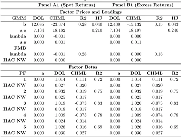
It follows from the previous section that the Corner Portfolio of the carry trade strategy (henceforth termed CHML for simplicity) should be tested as a candidate second factor for the pricing kernel. Panels A1 and B1 of Table 12 present the cross-sectional pricing results of the tests using the commodity portfolios 1-5 as test assets and DOL and CHML as factors.
The results indicate that the DOL factor is highly correlated with the returns of Portfolios 1-5. The betas on the DOL factor are all close to one in value, and statistically signi…cant. The betas of the CHML factor decline, although not monotonically, from 0.11 for Portfolio1 to 0.02 for Portfolio 5. They are statistically signi…cant for three out of …ve portfolios. While the R2s for the …ve regressions are large, this result is not surprising as sorting portfolios on the basis of the commodity price predictions produces a monotonic ordering of the expected returns. The R2s of the
cross-sectional regression are in the range of 0.28 but the factor risk price for CHML is negative.
5.3.2 The Volatility Proxy
Following Menkho¤ et al. (2012a) and Burnside, Eichenbaum and Rebelo (2011), I employ a measure of global currency volatility, denoted by VOL. The measure is e¤ectively the average sample standard deviation of the daily log changes in the values of the currencies versus the USD. It is measured monthly and is given by the following formula:
F X t = 1 Tt X 2Tt 2 4X k2K jrkj K 3 5 ’
where K denotes the number of available currencies on day and Tt denotes the total number
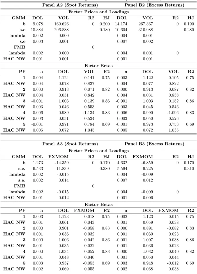
Keeping DOL as a …rst factor and replacing CHML by innovations to global FX volatility (hence-forth termed VOL) the pricing kernel yields the results detailed in Panels A2 and B2 of Table 12. The VOL factor does not fare well in terms of coe¢ cients’ signi…cance or monotonicity patterns for Portfolios 1-5. In addition, the cross-section results reveal that the VOL factor, clearly, does not price the cross section of commodity portfolio returns.
5.3.3 Exchange Rate Momentum
I further examine a momentum factor for the exchange rate. In line with the results of Menkho¤ et. al. (2012b), I form …ve portfolios on the basis of the currencies’ lagged returns over the past month which are held for one month. The constructed factor is essentially the momentum long-short portfolio i.e. Portfolio 5-Portfolio 1. The results for the Momentum Factor (FXMOM) are presented in Panels A3 and B3 of Table 12. Similarly to the Volatility Proxy, the Momentum Factor does not yield signi…cant coe¢ cients, neither does it price the cross-section of commodity portfolio returns.
TABLE 12 ABOUT HERE
5.3.4 The Fama-French Factors
Finally, a employ a comprehensive set of factors that relate to the equity market motivated by the …ndings of Chen and Tsay (2011). In particular, I collect six di¤erent factors computed on a daily basis from Kenneth French’s website and namely the Equity Market (MKT), Small minus Big (SMB), High minus Low (EHML), Equity Momentum (EMOM), Short-Term Reversal (STREV) and Long-Term Reversal (LTREV) factor. Table 13 summarizes the results of the asset pricing exercise when the Fama-French factors are employed.
The Fama-French factors, in general, fare a lot better than the standard exchange rate factors in explaining the cross section of commodity returns with the market factor being the best. In particular, the betas of the MKT factor decline, almost monotonically, from Portfolios 1 to Portfolio 5; furthermore, they are statistically signi…cant for three out of …ve portfolios. In addition, the R2 of the cross-sectional regression is large. Nevertheless, as in the case of CHML, the price of risk appears to be negative The SMB factor is probably the least successful, displaying little signi…cance and no patterns for portfolios 1-5 and no signi…cance and zero R2 in the cross section. EHML also fares poorly, while EMOM, on the other hand, gives good cross section results but provides less information in the individual portfolio regressions. Last but not least, STREV and LTREV appear to contain some information about the cross section of commodity returns while providing some meaningful spreads in the individual portfolio regressions.
TABLE 13 ABOUT HERE
However, despite the number of candidate variables examined, I do not manage to identify a risk factor that prices the cross section of the test assets, as the price of risk, , is never correctly signed and statistically signi…cant.
5.4 Discussion
The asset pricing results of the previous section appear rather inconclusive. Although it is possible to identify few factors that contain some information about the constructed commodity strategy, they tend to display a negative correlation with a plausible risk factor. Also, according to the results of the previous section, exchange rate returns stemming from a simple commodity strategy appear to be negatively related to the returns from other popular exchange rate strategies such as the carry trade. How does this …nding …t in the commodities literature?
Gorton and Rouwenhorst (2006) note that commodities display high Sharpe ratios and low cor-relations with other asset classes. They suggest that this argument is compatible with the theory of backwardation and market segmentation. Bessembinder and Chan (1992) further maintain that vari-ables that have predictive power over bond and stock returns and namely Treasury bill yields, equity dividend yield and the "junk" bond premium, are also able to forecast commodity returns. They attribute the negative correlation between commodities and other asset classes to a certain extent to di¤erent behaviour over the business cycle. Hence, it could be that the proposed commodity strategy appears to be unrelated to the equity market portfolio, as well as to the carry trade, because of this low correlation between commodities and equities, as well as between the short rate and commodity future returns respectively. This hypothesis is also in line with the …ndings of Büyük¸sahin, Haigh and Robe (2008), who report that commodities provide bene…ts to equity investors in terms of portfolio diversi…cation. The authors also …nd that even during the more recent years that investors have sought bigger exposure to commodities, there has not been an increase in the comovement between the returns on the two investments.
Last but not least, Frankel (2006) pushes for the existence of a negative relationship between interest rates and commodity prices. He argues that interest rates are transmitted into commodity currencies through the “extracting decision”, the carrying cost of inventories and through …nancial speculation in commodity markets
The issue, however, remains that the asset pricing exercise does not allow us to identify a priced factor of the proposed commodity strategy. In other words, the results indicate that the returns of
the strategy cannot be understood as compensation for risk. Therefore, the unconditional excess returns of the commodity strategy should either be attributed to some market ine¢ ciency or to existing limits to arbitrage. In this context, a mispricing story is also of relevance: when there is slow information di¤usion / limited attention, it takes time for information to be transmitted from one asset class to another (Daniel, Hirshleifer, and Teoh (2002), Hirshleifer and Teoh (2003) and Lim and Teoh (2010)). Since prices should eventually re‡ect full information, return predictability should fade away with the passage of time. My …ndings point towards this direction; return predictability holds at the daily level, but weakens signi…cantly at the weekly and monthly level. The empirical results of this paper are not adequate to fully address this issue; however, the following section further explores some of the aforementioned arguments.
6
Robustness
6.1 Sub-sample Analysis
In order to establish that my results are not driven by a spike in correlations during the global …nancial crisis, I divide the sample into two sub-samples around the crisis period. The …rst sub-sample contains observations up to the end of June 2007 and the second sub-sample contains observations between July 2007 until the end of the sample. I then calculate descriptive statistics for spot and excess returns as before. The descriptive statistics for the seven commodity portfolios are displayed in Tables 14 and 15 for the spot and excess return cases respectively. The results suggest that the monotonic ordering of the …ve portfolios persists across sub-samples. Additionally, the Sharpe Ratios of the strategies are higher in the post-crisis period for both the spot and excess returns series, indicating that the proposed strategy behaves as a fundamental strategy. Again, there is not a clear monotonic pattern regarding the standard deviations, and the skewness and kurtosis measures. However, once more, the extreme values with respect to the second, third and fourth moments consistently appear in Portfolios 1 and 5 for both sub-samples.
TABLES 14 & 15 ABOUT HERE
At this point, it would be also interesting to look at the coevolution of the spot and excess cumulative returns of the commodity strategy with the carry trade. Figure 2 is indicative of the previously detected negative relationship between the two strategies.
6.2 Exploitability of the Commodity Strategy
My analysis has so far ignored the exploitability of the proposed commodity strategy. This is an important concern given that the rebalancing frequency is daily and the employed currency universe includes emerging market currencies which are known to display high bid-ask spreads. In order to address this issue, I calculate net spot returns for the …ve portfolios based on the commodity strategy predictions, for all 25 currencies, by adjusting spot returns for bid-ask spreads. Following Goyal and Saretto (2009) and Menkho¤ et al. (2012), I employ the 50% of the quoted bid-ask spread as the actual spread. This is still a conservative choice given that Gilmore and Hayashi (2011) report that actual transaction costs stemming from bid-ask spreads probably constitute a lot less than 50% of the quoted bid-ask spread. Table 16 display the results of this exercise for spot and excess returns.
TABLE 16 ABOUT HERE
I …nd that, at …rst glance, it does not seem possible to exploit the information arising from the commodity strategy. The spot returns to Portfolios 1-5 are all negative and, hence, economically unappealing. In the light of these results, there does not appear to be any need to construct the corner portfolio as it will evidently be loss making. However, the inspection of Tables 18 and 19 reveals some additional information. In particular, the monotonicity of portfolio returns is slightly disrupted compared to the results of Table 7. Furthermore, Portfolio 1 appears to fare particularly badly when transaction costs are incorporated, for both the spot and excess return cases, indicating a higher participation of emerging market currencies.
Figures 3 and 4 indicate the relative participation of currencies in Portfolios 1 and 5. A …rst observation is that both portfolios are dominated by commodity exporters suggesting consistency of the strategy mechanics. The second remark pertains to the fact that emerging market currencies (such as the South African Rand, the Brazilian Real, the Chilean Peso and the Mexican Peso), which display on average higher bid-ask spreads, constitute a non-trivial portion of these portfolios.
FIGURES 2 & 3 ABOUT HERE
A natural step will therefore be to carry the analysis in the developed market space. This will act as an additional robustness check by showcasing whether the predictability of the commodity strategy is mainly driven by less liquid currencies, and most importantly, by shedding more light in the exploitability issue.
6.3 The Commodity Strategy in Developed Markets
For this part of the analysis, I restrict my currency universe to GBP, CHF, JPY, CAD, AUD, NZD, SEK, NOK, EUR, SGD, CZN, and HRK versus the USD. Again, I sort the currencies according to the forecasted returns of the commodity strategy and reallocate them to three portfolios this time, on a daily basis, for both the spot and excess return cases. Following the same logic as before, Portfolio 1 contains the currencies with the highest sell signal and Portfolio 3 contains the currencies with the highest buy signal. The Average Portfolio contains all the currencies and each portfolio is equally weighted. Given that the exploitability of the strategy is the key focus here, I also report spot and excess returns net of transaction costs. The results, displayed in Tables 17 and 18, paint a much brighter picture; not only is the commodity strategy valid for developed markets but one can also make a net excess return of 3 per cent annually by investing in the "long portfolio".
TABLES 17 & 18 ABOUT HERE
The portfolios again display monotonically increasing annualized returns when one moves from Portfolio 1 to Portfolio 3. The reported standard deviations are slightly higher compared to the benchmark case when all 25 currencies are employed. Although there is no clear skewness and kurtosis pattern, Portfolio 3 displays almost zero skewness and a coe¢ cient of kurtosis close to three, unlike Portfolio 1, the returns of which are positively skewed but leptokurtic.
In the case of developed markets, the number of test assets falls to three, undermining the validity of asset pricing tests. However, I look at the correlation of the …rst two principal components of the portfolio returns between the developed markets case and the full country panel is striking: The correlation between the …rst principal components amounts to 0.95 and the correlation between the second principal components is as high as 0.76. This points towards the direction that the nature of the returns in the full sample is similar to that in the developed markets case.
6.4 Extension: a Simple Market-Timing Exercise
Given the daily rebalancing and the high transaction costs of the strategy, it would be of great interest to see if an investor could pro…t by timing her trades, assuming in this case uncertainty risk. For this purpose, I study the return pro…le of a market-timing version of the commodity strategy, where the investor trades only if the expected return of the long-short strategy exceeds the observed transaction costs of the currencies involved, on the previous day. In this instance, the investor trades, roughly, two thirds of the time. The results for the excess returns case, net of transaction costs, are presented in Table 19.
TABLE 19 ABOUT HERE
The results indicate that the employment of this very simple rule makes it possible to recover the returns of the strategy after the incorporation of transaction costs. However, one must note that in this case the investor assumes additional uncertainty risk.
7
Conclusion
The present paper proposes a novel strategy for the exchange rate that employs changes in the global prices of tradable commodity indices to forecast currency returns, which I term “commodity strategy”. First, I document that commodity prices have signi…cant in-sample and out-of-sample forecasting ability for the future exchange rates of several commodity exporters and importers at the daily frequency. However, unlike some of the …ndings of the recent international …nance literature11, the reverse relationship appears to be weaker in-sample and does not survive out-of-sample testing. Second, I …nd a signi…cant cross-sectional spread in both spot and excess returns of 6% per annum between the currencies that are predicted to appreciate and those that are predicted to depreciate by the “commodity strategy”. At the same time, the returns appear to be uncorrelated to popular exchange rate strategies such as the carry trade and currency momentum. The strategy works across di¤erent sub-samples and fares particularly well during the crisis period - when carry trades collapsed - consistent with the behaviour of fundamental strategies which bene…t from the “‡ight to quality” during …nancial turmoils. The aforementioned …ndings have important implications for an investor’s currency portfolio allocation decisions, and the latter could bene…t from taking into account commodity price movements when investing in currencies.
The relationship between commodity prices and exchange rates is also found to be relevant for a broader set of currencies besides this of commodity currencies. I argue that this is consistent with the theory that commodity price ‡uctuations serve as an observable and exogenous terms-of-trade shock for a small open exporter or importer. Despite the emergence of potentially important variables, a priced factor for the proposed commodity strategy remains to be identi…ed. The empirical results of the present work fall sort of detecting the source of risk for which the investor gets compensated by the returns of the commodity strategy and future work in this area is highly encouraged, as factors such as the interest rate and the equity market appear to negatively correlate with the strategy returns. However, the impact of transaction costs is non-trivial; adjusting returns for bid-ask spreads can erode pro…tability completely when the strategy is implemented using a number of emerging market currencies which display large bid-ask spreads which act as barriers to arbitrage
1 1
activity. Nevertheless, the ordered portfolios need not necessarily be skewed towards currencies with high transaction costs; the investor can recover pro…tability, to some extent, by trading only developed market currencies. I also explore the exploitability issue by implementing a simple market timing rule. By trading roughly two thirds of the time I …nd that it possible to recover the returns of the strategy after the incorporation of transaction costs.
Given that return predictability holds at the daily level, but weakens signi…cantly at the weekly and monthly level, the issue of mispricing emerges as another possibility. In line with the literature of limited investor attention (Daniel, Hirshleifer, and Teoh (2002), Hirshleifer and Teoh (2003) and Lim and Teoh (2010)), it might be that it takes time for information to be transmitted from com-modity prices to exchange rates. This could be a plausible explanation for the documented return predictability; ultimately, the proposed strategy involves frequent rebalancing, while the existence of transaction costs acts as a barrier to arbitrage for a number of currencies. Since prices should eventually re‡ect full information, return predictability indeed fades away with the passage of time.
8
References
Amano, R., and van Norden S., 1993. A Forecasting Equation for the Canada-U.S. Dollar Exchange Rate. The Exchange Rate and the Economy (Ottawa: Bank of Canada).
Ang, A., Hodrick R., Xing Y., and Zhang X., 2006. The cross-section of volatility and expected returns. Journal of Finance, 61, 259-299.
Basher, S. A., Haug, A. A., & Sadorsky, P., 2010. Oil Prices, Exchange Rates and Emerging Stock Markets. Economics Discussion Papers Series No. 1014, Department of Economics, University of Otago.
Bessembinder, H. and Chan, K., 1992. Time-Varying Risk Premia and Forecastable Returns in Futures Markets. Journal of Financial Economics, 32, 169–193.
Büyük¸sahin, B., Haigh, M., and Robe, M., 2008. Commodities and Equities: A "Market of One? mimeo, U.S. Commodity Futures Trading Commission.
Cashin, P., Cespedes, L. F., and Sahay R., 2004. Commodity Currencies and the Real Exchange Rate. Journal of Development Economics, 75, 239-268.
Chen, Y., and Rogo¤, K. S., 2004. Commodity Currencies. Journal of International Economics 60, 133-169.
— — — — , Are the Commodity Currencies an Exception to the Rule? Global Journal of Economics, 1, 1250004.
Chen, Y., Rogo¤, K. S. and Rossi, B., 2010. Can Exchange Rates Forecast Commodity Prices? Quarterly Journal of Economics, 125, 1145–1194.
Chen, Y. and Tsay, W.,2011. Forecasting Commodity Prices with Mixed-Frequency Data: An OLS-Based Generalized ADL Approach. Working Paper.
Clements, K. W and Fry R., 2006. Commodity Currencies and Currency Commodities. Economics Discussion / Working Papers 06-17, The University of Western Australia.
Daniel K., Hirshleifer D., and Teoh S., 2002. Investor psychology in capital markets: Evidence and policy implications. Journal of Monetary Economics, 49, 139-209.
Ferraro, D., Rogo¤, K. and Rossi B., 2012. Can Oil Prices Forecast Exchange Rates? NBER Working Paper No. 17998.
Gilmore, S., and Hayashi F., 2011. Emerging market currency excess returns. American Economic Journal: Macroeconomics, 3, 85-111.
Gorton, G.and Rouwenhorst G., 2006. Facts and Fantasies about Commodity Futures. Financial Analysts Journal, 62, 47–68.
Goyal, A., and Saretto A., 2009. Cross-section of option returns and volatility. Journal of Financial Economics, 94, 310-326.
Gruen D. and Kortian T., 1996. Why Does the Australian Dollar Move so Closely with the Terms of Trade? RBA Research Discussion Papers rdp9601, Reserve Bank of Australia.
Hansen, L. P., and Jagannathan R., 1997, Assessing speci…cation errors in stochastic discount factor models, Journal of Finance, 52, 557-590.
Hirshleifer D. and Teoh S., 2003. Limited attention, information disclosure, and …nancial reporting. Journal of Accounting and Economics, 36, 337-386.
Lim S., and Teoh S., 2010. Limited attention. In Behavioral Finance: Investors, Corporations, and Markets. Editors Kent Baker and John Nofsinger, Robert Kolb Finance Series, John Wiley, 295-312.
Lustig H., Roussanov N. and Verdelhan A., 2011. Common Risk Factors in Currency Markets. Review of Financial Studies, 24, 3731-3777.
Lustig H. and Verdelhan A., 2007. The Cross-Section of Foreign Currency Risk Premia and US Consumption Growth Risk. American Economic Review, 97, 89-117.
Menkho¤ L., Sarno L., Schmeling M. and Schrimpf A., 2012a. Carry Trades and Global Foreign Exchange Volatility. Journal of Finance, 67, 681-718.
— — — –, 2012b. Currency Momentum Strategies, Journal of Financial Economics, 106, 660-684.
— — — –, 2013. The Cross-Section of Currency Order Flow Portfolios. Working Paper.
Newey, W., and West, K. D., 1987. A Simple, Positive Semi-De…nite, Heteroskedasticity and Autocorrelation Consistent Covariance Matrix. Econometrica, 55, 703-708.
Obstfeld, M., and Rogo¤, K., 1996. Foundations of International Macroeconomics. Cambridge, MA: MIT Press.
Obstfeld, M., and Rogo¤, K., 2000. The Six Major Puzzles in International Macroeconomics: Is There a Common Cause? In Bernanke, B. and Rogo¤, K. (eds.) NBER Macroeconomics Annual, Cambridge: MIT Press, 339-390.
Ready R., Roussanov N. and Ward C., 2013. Commodity Trade and the Carry Trade: A Tale of Two Countries. NBER Working Paper.
Sarno L. and Valente G., 2009. Exchange rates and fundamentals: Footloose or evolving relation-ship? Journal of the European Economic Association, 7, 786–830.
Taylor A., 2001. Potential Pitfalls for the “Purchasing-Power-Parity Puzzle? Sampling and Speci-…cation Biases in Mean Reversion Tests of the Law of One Price. Econometrica, 69, 473-498.
Table 1: Countries and Commodities
Country Commodity Indices
Australia Gold Wheat Aluminium Brent
0.25*** 0.09*** 0.23*** 0.12***
Brazil Agriculturals Brent
0.15*** 0.10***
Bulgaria Copper Energy Brent
0.09*** 0.06*** 0.05***
Canada Natural Gas Brent
0.02*** 0.09***
Chile Copper Brent
0.12*** 0.04***
Croatia Natural Gas Brent
0.01** 0.06***
Czech Republic Brent
0.08***
Germany Brent
0.06***
Hungary Brent
0.10***
India Precious Metals Brent
0.05*** 0.03***
Indonesia Natural Gas Brent
0.01* 0.02***
Israel Brent
0.03***
Japan Brent
-0.02*
Mexico Silver Brent
0.07*** 0.07***
New Zealand Livestock Aluminium Brent
0.09*** 0.20*** 0.10***
Norway Natural Gas Industrial Metals Brent
0.02*** 0.19*** 0.11***
Philippines Brent
0.02***
Poland Brent
0.10***
Russian Federation Natural Gas Brent
0.01** 0.05***
Singapore Brent
0.04***
South Africa Gold Brent
0.28*** 0.11***
Sweden Brent
0.10*
Switzerland Industrial Metals Brent
0.09*** 0.04***
Thailand Brent
0.01***
United Kingdom Brent
0.06***
This table presents the commodities that form a 5% (or greater) share of a country’s GDP, according to data collected from the United Nations Commodity Trade Statistics Database, for which there exist tradable commodity index series.Asterisks denote statistical signi…cance at the 1% (***), 5% (**) and
Table 2: Currency Beta Rankings versus the USD and GBP CURRENCY BETA CURRENCY BETA USD_AUD 0.184*** GBP_BRL 0.150*** USD_ZAR 0.168*** GBP_AUD 0.127*** USD_PLN 0.165*** GBP_MXN 0.127*** USD_HUF 0.161*** GBP_CAD 0.125*** USD_NZD 0.155*** GBP_ZAR 0.123*** USD_BRL 0.150*** GBP_PLN 0.101*** USD_NOK 0.146*** GBP_CLP 0.101*** USD_SEK 0.142*** GBP_NZD 0.096*** USD_CAD 0.131*** GBP_RUB 0.091*** USD_CZN 0.123*** GBP_NOK 0.085*** USD_MXN 0.104*** GBP_HUF 0.084*** USD_HRK 0.091*** GBP_SEK 0.080*** USD_GBP 0.090*** GBP_INR 0.078*** USD_BGN 0.089*** GBP_SGD 0.075*** USD_EUR 0.089*** GBP_PHP 0.073*** USD_CLP 0.081*** GBP_IDR 0.073*** USD_RUB 0.073*** GBP_ILS 0.069*** USD_CHF 0.059*** GBP_THB 0.065*** USD_SGD 0.052*** GBP_CZN 0.063*** USD_INR 0.042*** GBP_GBP 0.059*** USD_ILS 0.041*** GBP_HRK 0.043*** USD_IDR 0.033*** GBP_BGN 0.041*** USD_PHP 0.030*** GBP_EUR 0.040*** USD_THB 0.023*** GBP_CHF 0.024*** USD_JPY -0.022* GBP_JPY 0.016
This table presents the rankings of the currencies versus the USD (left panel) and the GBP (right panel) according to the betas from the regression of the nominal exchange rates on the GSCI index. Asterisks denote statistical signi…cance at the 1% (***), 5% (**) and 10% (*) level. Returns are daily and the sample period is 01/2000-11/2011.
Table 3: Pairwise Granger-Causality Tests: Commodities to Currencies
Country Commodity Indices
Australia Gold Wheat Aluminium Brent
0.004*** 0.002*** 0.062* 0.159
Brazil Agriculturals Brent
0.012** 0.239
Bulgaria Copper Energy Brent
0.072* 0.173 0.477
Canada Natural Gas Brent
0.182 0.013**
Chile Copper Brent
0.221 0.268
Croatia Natural Gas Brent
0.058* 0.092*
Czech Republic Brent
0.830
Germany Brent
0.560
Hungary Brent
0.855
India Precious Metals Brent
0.000* 0.046**
Indonesia Natural Gas Brent
0.201 0.000***
Israel Brent
0.026**
Japan Brent
0.218
Mexico Silver Brent
0.682 0.006***
New Zealand Livestock Aluminium Brent
0.805 0.679 0.444
Norway Natural Gas Industrial Metals Brent
0.052* 0.260 0.001***
Philippines Brent
0.001***
Poland Brent
0.394
Russian Federation Natural Gas Brent
0.295 0.003***
Singapore Brent
0.005***
South Africa Gold Brent
0.562 0.989
Sweden Brent
0.371
Switzerland Industrial Metals Brent
0.542 0.697
Thailand Brent
0.049**
United Kingdom Brent
0.092*
This table reports p-values for the Granger-causality test. Asterisks denote rejection at the 1% (***), 5% (**) and 10% (*) signi…cance levels respectively of the null hypothesis that commodity price changes29
Table 4: Out-of-Sample Predictive Ability: Commodities to Currencies
MSFE Di¤erence Between the "Commodity Price Model" and the Random Walk
Country Australia Poland Hungary Sweden Norway
MSFE di¤erence 0.025 0.030* 0.024 0.024 0.036**
t-statistic 1.202 1.562 1.273 1.093 1.815
Country Czech Republic New Zealand South Africa Germany Bulgaria
MSFE di¤erence 0.021 0.019 0.001 0.029* 0.043**
t-statistic 0.999 0.936 0.051 1.380 2.047
Country Canada Croatia Indonesia Mexico Brazil
MSFE di¤erence 0.037** 0.057*** 0.058*** 0.028** 0.054***
t-statistic 1.759 2.760 2.775 1.364 2.608
Country Switzerland Russian Federation Chile Israel India
MSFE di¤erence 0.015 0.105*** 0.052*** 0.040** 0.094***
t-statistic 0.735 5.027 2.480 1.906 4.529
Country Singapore Thailand Philippines United Kingdom Japan
MSFE di¤erence 0.025 0.031* 0.091*** 0.048** 0.010
t-statistic 1.185 1.489 4.351 2.319 0.470
The table reports re-scaled MSFE di¤erences between the model and the random walk forecasts. Positive values imply that the model forecasts better than the random walk. Asterisks denote rejections of the null hypothesis that random walk is better in favour of the alternative hypothesis that the commodity-based model is better. Asterisks denote rejection at the 1% (***), 5% (**) and 10% (*) signi…cance levels respectively. Clark and West (2006) t-statistics are also presented below (one-sided test)