Abstract: Bottom friction modeling is an important step in river flows computation with 1D or 2D solvers. It is usually performed using empirical laws established for uniform flow conditions or a modern approach based on turbulence analysis.
Following the definition of the flow validity field of the main friction laws proposed in the literature, an original continuous formulation has been developed. It is suited to model river flows with a high variability of properties (water depth, discharge, roughness…).
The efficiency of this new formulation, theoretically established and numerically adjusted, is demonstrated through various practical applications.
Keywords: Shallow water, Bottom friction, Empirical laws,
Modern laws
I.INTRODUCTION
Shallow Water equations are commonly used to model numerically river flows. Indeed, their only assumption states that the flow velocity component normal to the main flow plane is smaller than the flow velocity components in this plane. This is the case for the majority of river flows where vertical velocity component is negligible regarding the horizontal ones, except in the vicinity of singularities such as weirs for example.
This paper focuses on bottom friction modeling in such mathematical models. This effect is indeed of very high importance for real flow computation despite it is generally evaluated from empirical formulations experimentally determined for ideal uniform flows.
The bottom friction term should represent the whole of the energy losses induced by the friction of the fluid on the rough river bed. It is thus related to the bed characteristics (shape, roughness), to the fluid characteristics (viscosity) and to the flow features (water height, velocity).
The concept of friction slope has been early used to characterize bottom friction. It is an non-dimensional number corresponding to the slope to give to a uniform channel to observe a uniform flow for a given discharge. This concept is at the basis of the first friction laws proposed in the second part of the 18th century by the researchers of the so called “empirical” school. Authors such as Chézy and Manning proposed laws based on experimental results consisting in measuring the friction slope for varied idealized flows in a laboratory flume. A second approach appeared later following works of Prandtl. It provided laws issued from a scientific reasoning on the physics of the shear layer phenomena. It is the “modern” school.
Today, both approaches are used by free surface flow modelers, and these laws are sometimes applied to flow
conditions far from those on the basis of which they have been developed.
The aims of the developments presented in this paper were to define the validity fields of varied bottom friction formulations proposed in the literature, and to find a single law usable to describe the bottom friction phenomena for largely variable flow conditions.
II.MAIN FRICTION LAWS
The large range of bottom friction formulations proposed in the literature can be divided into two parts: the empirical and the modern approaches.
The first ones have been defined from experimental results in idealized uniform channel and for uniform flows. It’s thus important to know the assumptions and the experimental conditions which are at the basis of the formula elaboration.
The second ones are based on theoretical developments related to the physics of the friction phenomena. The structure of these modern formulations is thus more congruent with the laws of fluids mechanics.
The main formulations of these two schools are summarized in this paragraph with the reasoning leading to their elaboration.
A.Empirical laws
The laws of the so called “empirical” school have all been developed on the basis of experimental tests. These tests consisted in measuring the slope to give to a uniform channel to observe a uniform flow [1]. In these flow conditions, the effects of bottom friction are exactly counterbalanced by the gravitational forces. Thus the friction slope is equal to the bottom slope of the channel and simple formulae can be set up to link the channel roughness, the flow variables and the bottom slope. Replacing the bottom slope by the friction slope, the friction effects can be computed for other flow conditions than the uniform ones.
The general form of empirical friction formulations writes:
χ
α
J
R
hU
=
12 (1)It relates the friction slope J to hydraulic and geometric parameters affecting the bottom friction such as U the mean flow velocity, α a friction coefficient and Rh the hydraulic
radius. This last parameter reflects the effect of the cross section shape.
The difference between the different friction formulations of the empirical school is in the χ exponent value and in the α coefficient form.
Bottom friction formulations for free surface flow modeling
Machiels Olivier1, Erpicum Sébastien1, Archambeau Pierre1, Dewals Benjamin1, 2, Pirotton Michel1 1 Université de Liège – Département ArGEnCo, Unité de recherche HACH
Chemin des chevreuils 1, B52/3 – 4000 Liège 2 Fond National de la Recherche Scientifique (FRS-FNRS)
email: [email protected], [email protected], [email protected], [email protected], [email protected]
It is important to note that these formulations are not explicitly dependent on the turbulence regime of the flow, despite it is well known this flow state is of great influence on the friction losses.
The first empirical friction law has been proposed by Chézy in 1775 [2], when this engineer had to determine the cross section of channels necessary to provide water to the city of Paris. It writes: 2 1 2 1 h
R
CJ
U
=
(2)where C is the roughness coefficient, for which different authors such as Bazin [3], Ganguillet and Kutter [4] proposed formulations function of the shape and the nature of the channel bed.
Another remarkable law is the one developed by Manning in 1919 [5]. It writes: 3 2 2 1
1
hR
J
n
U
=
(3)where n is the Manning’s coefficient relating the effects of the bottom roughness.
The success of the Manning’s formulation is mainly due to the Strickler’s relation [6] to define the roughness coefficient. Strickler studied the value of the bottom roughness coefficient
K and defined a relation directly related to the size of the
roughness elements d. 6 1
26
1
d
n
K
=
=
(4)Varied literature sources provide values for K coefficient depending on flow conditions as well as the shape and the nature of channels or rivers beds.
Chézy and Manning-Strickler formulations are the most widely used empirical friction laws. Others exist, based on the same assumptions, such as the laws of Gauckler, Forchheimer, Christen, Hagen and Tillman [1]. They differ only by the exponent of the hydraulic radius in the general formulation (1) (Table I).
TABLEI
VALUE OF
χ
EXPONENT OF THE HYDRAULIC RADIUS FORDIFFERENT EMPIRICAL FRICTION FORMULATIONS [1]
Author χ Gauckler 0.4 Forchheimer 0.7 Christen 0.625 Hagen 0.714 Tillman 0.7 B.Modern school
At the opposite of the empirical laws, the formulations from the modern school are based on a theoretical reasoning on the physics of the friction phenomena [1].
The developments of the modern school appear one century later than the first empirical development. That is at the start of the 20th century that, under the leadership of Prandtl, many researchers from the University of Göttingen (Germany) developed formulations of a friction coefficient, λ, function of
the turbulence of the flow through the Reynolds number Re, and the size of the roughness elements of a pipe, k.
Modern formulations have been initially developed for pressurized flows to determine head losses along a pipe.
The Darcy-Weisbach relation [7] allows to link the friction slope J to the friction coefficient λ:
g
U
R
J
h2
4
2λ
=
(5)where 4 Rh is the equivalent diameter of a channel regarding
pressurized flows and g is de gravity acceleration.
The friction coefficient λ evaluation depends on the flow turbulence regime, and thus the Reynolds.
1) Laminar regime
The friction coefficient variation in laminar flows (Re < 5000) has been described by Poiseuille [8]:
Re
64
=
λ
(6)For this flow regime, the roughness of the pipe has no effects on the flow as it’s in laminar conditions.
2) Smooth turbulent regime
In turbulent regime, the effect of the size of the roughness elements on friction depends of the Re value.
Prandtl expressed the variation of the friction coefficient λ for flows on smooth walls in the Prandtl-Von Karman formulation [9]:
λ
λ
Re
.
log
2
51
2
1
=
−
(7)This formulation is a simple function of the state of the fluid such as (6). Indeed, on smooth walls, the size of the roughness elements is negligible compared to the size of the laminar boundary layer.
In the same scope, Blasius [10] proposed an explicit formulation of the friction coefficient for flows on smooth walls: 4 1
3164
0
Re
.
=
λ
(8)It fits well to Prandtl results for Re lower than 105.
3) Rough turbulent regime
The rough turbulent regime is defined by a ratio between the Reynolds number, Re, and the relative roughness, k/Rh.
Indeed, more turbulent is the flow, smaller is the laminar boundary layer and more important is the effect of the wall roughness on the flow.
The rough turbulent regime appears when the effects of the roughness are predominant, i.e. for values of the Reynolds number higher than a limit value ReLim defined by:
k
R
Re
hLim
=
2240
(9)For this regime, Nikuradse [11] developed an explicit formulation of the friction coefficient λ function of the relative roughness k/Rh: h
R
k
8
.
14
log
2
1
=
−
λ
(10)4) Transitional regime
The transitional regime is the regime between the smooth and the rough turbulent ones. Colebrook [12] proposed a formulation of the friction coefficient by combining the Nikuradse (10) and the Prandtl (7) formulations:
⎟⎟
⎠
⎞
⎜⎜
⎝
⎛
+
−
=
λ
λ
Re
.
R
.
k
log
h51
2
8
14
2
1
(11) The implicit character of this equation gives it an uneasily use. It is the reason why different authors tried to find an explicit equivalent formulation, such as Barr [13, 14] and Yen [15]. The second law of Barr provides the best results regarding the Colebrook formulation (11), with less than 1% error on the friction coefficient values:⎟⎟ ⎟ ⎟ ⎟ ⎟ ⎟ ⎟ ⎟ ⎟ ⎟ ⎟ ⎟ ⎠ ⎞ ⎜⎜ ⎜ ⎜ ⎜ ⎜ ⎜ ⎜ ⎜ ⎜ ⎜ ⎜ ⎜ ⎝ ⎛ ⎟ ⎟ ⎟ ⎟ ⎟ ⎠ ⎞ ⎜ ⎜ ⎜ ⎜ ⎜ ⎝ ⎛ ⎟⎟ ⎠ ⎞ ⎜⎜ ⎝ ⎛ + ⎟ ⎠ ⎞ ⎜ ⎝ ⎛ + − = 53 76 1 7 518 4 8 14 2 1 7 0 52 0 . R k Re Re Re log . R . k log . h . h λ (12) 5) Macro-roughness
Macro-roughness is considered when the size of the roughness elements becomes comparable to the water depth h.
h
k
Lim=
0
.
25
(13)Developments on macro-roughness are more recent and are directly related to the development of hydrological modeling. They are associated to the modern school because of the similar form of the mathematical formulations.
The formulation of Bathurst [16], developed in 1985, is a reference to study flows on macro-roughness:
h
k
15
.
5
log
987
.
1
1
=
−
λ
(14)The formulation of Dubois [17] can also be cited. Based on the same form of Bathurst’s law, this formulation takes into account the density p of the roughness elements:
613 . 0
13
.
3
log
62
.
5
8
=
+
p
−k
h
λ
(15)In 2D flow modeling, the hydraulic radius Rh is equivalent
to the water depth h. In the rest of this paper, both expressions will be used similarly.
III.VALIDITY FIELDS OF THE EMPIRICAL LAWS
On the other hand, the empirical laws have not been developed regarding the variation in turbulence regime of real water flows. All of them have been defined in the scope of specific applications and for fixed uniform flow conditions. On the other hand, modern laws take better into account the turbulence regime of the flow but none of them can be applied to the whole flow conditions of real river flows. In this paragraph, the validity field of the main empirical laws is defined regarding the friction losses values provided by the
different modern laws depending on the flow turbulence regime.
For laminar flows, the Poiseuille law (6) can be written, using the Darcy-Weisbach relation (5), such as:
h
JR
Re
g
U
8
=
(16)This equation is similar to the general form of empirical laws. For laminar flow condition:
8
5
0
Re
g
.
=
=
α
χ
(17) Thus, only Chézy’s formulation with an adapted value of αcan model friction losses in laminar conditions.
In the smooth turbulent regime, Prandtl’s law (7) has to be considered. Its implicit form makes the comparison more difficult, but, as the law is independent of the hydraulic radius, the empirical like formulation of equations (5) and (7) is similar to equation (16) and thus χ has to be equal to 0.5 again. Thus, Chézy’s formulation is again the only law suited to model friction losses in the smooth turbulent regime.
Blasius formulation can be used to set another empirical like formulation in smooth turbulent regime:
h
JR
Re
g
.
U
=
25
3
14 (18)In rough turbulent regime, the Nikuradse formulation (10) is a complex function of the hydraulic radius, Rh. Inserted in
the Darcy-Weisbach relation (5), the modern law cannot be compared directly with the empirical formulations. This problem can be solved by replacing the logarithm of the relative roughness by its power development. The empirical like formulation of equation (5) and (16) writes then:
( ) ( )
( )( )
⎪ ⎪ ⎩ ⎪ ⎪ ⎨ ⎧ ⎟ ⎠ ⎞ ⎜ ⎝ ⎛ = ⎥ ⎦ ⎤ ⎢ ⎣ ⎡ ⎟⎟ ⎠ ⎞ ⎜⎜ ⎝ ⎛ − = = ⎟ ⎠ ⎞ ⎜ ⎝ ⎛ − + − k R M R k k R A R J Ak g U h k R h h M h M h 8 . 14 log 2 10 ln 8 . 14 log 2 with 8 8 . 14 log 10 ln 2 1 2 1 2 1 2 1 2 1 (19)The empirical laws are thus valid for rough turbulent regime if the double equality (20) is satisfied:
( )
⎪ ⎪ ⎩ ⎪⎪ ⎨ ⎧ = + = M Ak g M 1 8 2 1 2 1α
χ
(20)The first equality can be satisfied for each value of the hydraulic radius exponent χ but for a particular value of the relative roughness k/Rh.
For χ = 0.5, the coefficient M value must be infinity. This means that the relative roughness has be 0. So the Chézy’s formulation is a limit to the bottom friction evaluation in turbulent regime in case of smooth bed. The formulations with χ value lower than 0.5 are not valid in this specific flow regime.
In the Manning’s formulation, with χ = 0.667, the value of
evaluated for a relative roughness equal to 0.037. In this case, the Strickler coefficient is equal to:
6 1 613 . 26 k K = (21)
This value is very close to the Strickler formulation (4). For other empirical laws using an exponent χ higher than 0.5, the same calculations can be performed. Each of these laws is thus suited to describe correctly the bottom friction phenomena for a specific value of the relative roughness and a particular form of the α coefficient (Table II).
TABLEII
VALUE OF RELATIVE ROUGHNESS AND COEFFICIENT α FOR A SUITABLE DESCRIPTION OF THE BOTTOM FRICTION EFFECTS IN
ROUGH TURBULENT REGIME
Author χ k/Rh α Christen 0.625 0.005 31.71/k0.125 Manning 0.667 0.037 26.61/k0.167 Tillman 0.7 0.1 24.26/k0.2 Forchheimer 0.7 0.1 24.26/k0.2 Hagen 0.714 0.138 23.51/k0.214
Considering the whole of the empirical laws, the bottom friction in rough turbulent flows can be correctly evaluated for relative roughness until 0.2. This last value is near the limit of macro-roughness. However, each law considered separately is only valid for a single relative roughness value, and none is thus available for general use.
The same developments as for the Nikuradse’s formulation can be performed with the Colebrook’s one. However, the coefficients A and M become also a function of the Reynolds number and thus of the state of the flow:
( ) ⎟ ⎟ ⎟ ⎟ ⎟ ⎠ ⎞ ⎜ ⎜ ⎜ ⎜ ⎜ ⎝ ⎛ ⎟⎟ ⎠ ⎞ ⎜⎜ ⎝ ⎛ + ⎟ ⎟ ⎟ ⎟ ⎟ ⎠ ⎞ ⎜ ⎜ ⎜ ⎜ ⎜ ⎝ ⎛ ⎟⎟ ⎠ ⎞ ⎜⎜ ⎝ ⎛ + − = ⎟⎟ ⎟ ⎟ ⎟ ⎟ ⎠ ⎞ ⎜⎜ ⎜ ⎜ ⎜ ⎜ ⎝ ⎛ ⎟ ⎟ ⎟ ⎟ ⎟ ⎠ ⎞ ⎜ ⎜ ⎜ ⎜ ⎜ ⎝ ⎛ ⎟⎟ ⎠ ⎞ ⎜⎜ ⎝ ⎛ + − = +1 2 1 2 1 2 1 2 1 574 18 5 0 10 51 2 8 14 51 2 8 14 2 M h M M h h M h h h R k A Re . . ln R k A Re . R . k log M R k A Re . R . k log k R A (22)
The empirical laws are again valid to predict the bottom friction value if the double equality of equation (20) is verified.
The Chézy’s formulation is still a limit for smooth bed and the laws with χ exponent value lower than 0.5 are not valid for transitional regime.
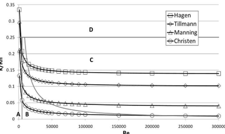
The other empirical formulations are valid for a single value of the relative roughness. However, this value varies with the Reynolds number (Fig. 1).
0 0.05 0.1 0.15 0.2 0.25 0.3 0.35 0 50000 100000 150000 200000 250000 300000 k/ R h Re Hagen Tillmann Manning Christen A B C D
Fig. 1. Value of relative roughness for a correct description of the bottom friction value in transitional regime – B (laminar –
A, rough turbulent – C, macro-roughness – D). As for the rough turbulent regime, the bottom friction value for transitional flows can be correctly evaluated with empirical laws for specific flow condition but none of the laws is of universal application.
Finally, for macro-roughness, the same reasoning can be applied than for the rough turbulent regime. Coefficients A and M are defined such as:
( )
( )
⎟ ⎠ ⎞ ⎜ ⎝ ⎛ = ⎥ ⎦ ⎤ ⎢ ⎣ ⎡ ⎟ ⎠ ⎞ ⎜ ⎝ ⎛ − = ⎟ ⎠ ⎞ ⎜ ⎝ ⎛ − k h M h k k h A k h 15 . 5 log 2 10 ln 15 . 5 log 987 . 1 15 . 5 log 10 ln (23)They are not a function of the flow regime.
As no empirical law is valid for relative roughness higher than 0.2, none of them is applicable to macro-roughness.
IV.USING FIELDS OF THE FRICTION LAWS
As a result of the study here above, a choice of friction law for modeling could be done depending on the flow conditions (Table III) [18].
When an explicit formulation is available to describe correctly the friction phenomena for particular flow conditions, it has been preferred to the corresponding implicit modern law.
TABLEIII
FRICTION LAWS USABLE FOR AN EFFICIENT MODELING OF THE FRICTION PHENOMENA
Fixed flow conditions
Variable flow conditions Laminar Poiseuille Chézy or Poiseuille Chézy or
Turbulent
Smooth Chézy or Prandtl Chézy or Prandtl Transitional Empirical laws (ex : Manning) Colebrook
Rough Empirical laws (ex : Manning) Nikuradse
V.EXTENSION OF THE EMPIRICAL LAWS VALIDITY FIELDS
To define more precisely the true validity field of the different empirical friction laws compared to the modern ones, it is necessary to define an acceptable error for friction losses evaluation between both approaches. The following developments consider that an error of 5% is acceptable on the water depth evaluation, defined as:
modern empirical modern
h
h
h
h
h
=
−
Δ
(24) For example, considering the Colebrook’s formulation, thewater depth is computed, using equation (5), as: M
h
k
A
gJ
U
h
1 2 Colebrook8
−⎟
⎠
⎞
⎜
⎝
⎛
=
(25)Regarding the study of the rough turbulent regime, the α coefficient (1) could be expressed as a function of the roughness: 2 1 −
=
χα
k
B
(26) where B is a constant parameter.By extension of this value for all turbulent flows, the water depth computed by the empirical laws can then be evaluated, using the equation (1), as:
χ 2 1 2 2 empirical −
⎟
⎠
⎞
⎜
⎝
⎛
=
h
k
J
B
U
h
(27)Using the water depths computed by the Colebrook formulation (25) and by the empirical laws (27) in (24), it is formal that this error is only function of the relative roughness. Validity fields of the friction laws for the description of transitional regime can thus be defined in terms of relative roughness (Table IV) [18].
TABLEIV
VALIDITY FIELDS OF THE PRINCIPAL FRICTION LAWS IN TERMS OF RELATIVE ROUGHNESS
Author Validity field (k/h) Chézy 0 Christen [0 ; 0.032] Manning [0.007 ; 0.1] Tillman [0.023 ; 0.29] Hagen [0.034 ; 0.38] Gauckler No validity Poiseuille Only laminar Prandtl 0 Colebrook [0 ; 0.1]
Barr [0 ; 0.1] Nikuradse [0 ; 0.1] Bathurst [0.1 ; 5.15]
The limit values of these validity fields are actually function of the Reynolds number. However, the variations are negligible for usual values of Reynolds for river flows (Re > 5000).
The higher terms of the validity fields of the Tillman and Hagen laws have been determined by comparison with the Bathurst formulation (14) because they concern macro-roughness.
The limitation of the macro-roughness has been extended to relative roughness of 0.1. It’s the results of a comparison, presented in paragraph VII, between modeling results and in situ measurements on river.
Today, the empirical laws of Manning and Chézy are the most widely used formulations for friction modeling. This success comes from their using simplicity and the large existing literature on their parameters values. However, the modern laws are more representative of the physics of bottom friction. Furthermore, explicit forms of the modern laws exist such as the one of Barr (12). The modern laws have thus an important interest for flow modeling.
In practice, other losses, such as these due to the turbulence, are included in the friction term used by most flow solvers. In this case, it is then important to keep in mind that the friction slope J represents not only the bottom friction phenomenon.
VI.LOOKING FOR A CONTINUOUS FRICTION FORMULATION
Regarding the validity fields of the empirical and modern laws (Table IV), it is remarkable that it doesn’t exist a single formulation suited to compute friction effects on the wide range of relative roughness encounter in real river flow, where h goes from 0 on the banks to several meters in the channel center with constant roughness height k. However, the k/h ranges of several laws are contiguous such as for example for Colebrook or Barr and Bathurst.
To solve this problem, an original approach has been developed on the basis of the three following statements:
− The Colebrook or Barr formulation is suited to model turbulent flows with relative roughness k/h lower than 0.1.
− The Bathurst formulation is suited to compute friction effect on macro-roughness, i.e. for k/h higher than 0.1.
− But these two formulations are not equal for a relative roughness k/h of 0.1.
Developments have been performed to link continuously these two formulations close to relative roughness k/h equal to 0.1.
Due to its explicit expression, the Barr’s formulation has been preferred to the Colebrook one.
To link the laws of Barr (12) and Bathurst (14), a third degree polynomial expression of the relative roughness has been set up:
D
h
k
C
h
k
B
h
k
A
⎟
+
⎠
⎞
⎜
⎝
⎛
+
⎟
⎠
⎞
⎜
⎝
⎛
+
⎟
⎠
⎞
⎜
⎝
⎛
=
2 31
λ
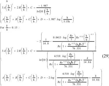
(28)The limits of application range of the different formulations have been choosen to ensure that the relative variation of the λ coefficient stays lower than 0.5 for a water depth variation of 1 cm. This condition allows to ensure the stability of traditional solvers. So, the equation (28) has been developed for k/h values between 0.05 and 0.15.
The parameters A, B, C and D values have been determined to get a continuous variation of λ (same value and tangent)
between the polynomial, the Barr and the Bathurst expressions at each limit of k/h range. Parameters A, B, C and
D have thus to solve the following complex system,
depending on Re: ( ) ( ) ( ) ( ) ( ) ⎪ ⎪ ⎪ ⎪ ⎪ ⎪ ⎪ ⎪ ⎪ ⎩ ⎪ ⎪ ⎪ ⎪ ⎪ ⎪ ⎪ ⎪ ⎪ ⎨ ⎧ ⎟ ⎟ ⎟ ⎟ ⎟ ⎠ ⎞ ⎜ ⎜ ⎜ ⎜ ⎜ ⎝ ⎛ + ⎟⎟ ⎠ ⎞ ⎜⎜ ⎝ ⎛ + ⎟ ⎠ ⎞ ⎜ ⎝ ⎛ − = + ⎟ ⎠ ⎞ ⎜ ⎝ ⎛ + ⎟ ⎠ ⎞ ⎜ ⎝ ⎛ + ⎟ ⎠ ⎞ ⎜ ⎝ ⎛ ⎟ ⎟ ⎟ ⎟ ⎟ ⎠ ⎞ ⎜ ⎜ ⎜ ⎜ ⎜ ⎝ ⎛ + ⎟⎟ ⎠ ⎞ ⎜⎜ ⎝ ⎛ + ⎟ ⎠ ⎞ ⎜ ⎝ ⎛ ⎟⎟ ⎟ ⎟ ⎟ ⎟ ⎠ ⎞ ⎜⎜ ⎜ ⎜ ⎜ ⎜ ⎝ ⎛ ⎟⎟ ⎠ ⎞ ⎜⎜ ⎝ ⎛ + ⎟ ⎠ ⎞ ⎜ ⎝ ⎛ ⎟ ⎠ ⎞ ⎜ ⎝ ⎛ − − = + ⎟ ⎠ ⎞ ⎜ ⎝ ⎛ + ⎟ ⎠ ⎞ ⎜ ⎝ ⎛ = ⎪ ⎪ ⎪ ⎩ ⎪⎪ ⎪ ⎨ ⎧ ⎟ ⎠ ⎞ ⎜ ⎝ ⎛ − = + ⎟ ⎠ ⎞ ⎜ ⎝ ⎛ + ⎟ ⎠ ⎞ ⎜ ⎝ ⎛ + ⎟ ⎠ ⎞ ⎜ ⎝ ⎛ ⎟ ⎠ ⎞ ⎜ ⎝ ⎛ − = + ⎟ ⎠ ⎞ ⎜ ⎝ ⎛ + ⎟ ⎠ ⎞ ⎜ ⎝ ⎛ = − h . k . Re Re Re log log D C B A h . k . Re Re Re log ln . Re Re Re Re log . . C B A : . h k log . D C B A ln . C B A : . h k . . . . . . . . 8 14 531 76 h k 1 7 4.518 2 h k h k h k 8 14 531 76 h k 1 7 4.518 10 531 76 h k 1 h k 7 0413 0 8 14 1 2 h k 2 h k 3 15 0 For 5.15h k 987 1 h k h k h k h k 10 987 1 h k 2 h k 3 05 0 For 7 0 52 0 2 3 7 0 52 0 2 7 0 52 0 3 0 52 0 2 2 3 2 (29)
However, for Reynolds numbers higher than 5000, which characterize most of usual river flows in the range of k/h ratio between 0.05 and 0.15, the variation of the parameters values with Re is negligible. The final form of the polynomial expression can then been established with constant parameters values: 22 . 5 89 . 9 83 . 382 76 . 1469 1 3 2 + ⎟ ⎠ ⎞ ⎜ ⎝ ⎛ + ⎟ ⎠ ⎞ ⎜ ⎝ ⎛ − ⎟ ⎠ ⎞ ⎜ ⎝ ⎛ = h k h k h k λ (30)
and the following expressions can be used to compute continuously the bottom friction effects in rivers or channels whatever the variation of k/h:
( )
⎟ ⎠ ⎞ ⎜ ⎝ ⎛ − = ≥ + ⎟ ⎠ ⎞ ⎜ ⎝ ⎛ + ⎟ ⎠ ⎞ ⎜ ⎝ ⎛ − ⎟ ⎠ ⎞ ⎜ ⎝ ⎛ = ≤ ≤ ⎟ ⎟ ⎟ ⎟ ⎟ ⎠ ⎞ ⎜ ⎜ ⎜ ⎜ ⎜ ⎝ ⎛ + ⎟ ⎟ ⎠ ⎞ ⎜ ⎜ ⎝ ⎛ + ⎟ ⎠ ⎞ ⎜ ⎝ ⎛ − = ≤ h . k log . . h k . h k . h k . h k . . h k . h . k . h k Re Re Re log . log . h k . . 15 5 987 1 1 : 15 0 For 22 5 89 9 83 382 76 1469 1 : 15 0 05 0 For 8 14 531 76 1 7 518 4 2 1 : 05 0 For 2 3 7 0 52 0 λ λ λ (31) VII.VALIDATIONTwo Belgian river reaches have been considered to validate the continuous approach: the Ourthe near the town of Hamoir and the Semois near Membre. These two reaches of 2.6 km and 1.6 km have been selected because of the presence of two water depth measurement stations on both of them. The downstream water depth measurement combined with the
discharge measurement provides the necessary boundary conditions for river reach modeling in case of subcritical flow.
The two river reaches have been modeled using the 2D-horizontal flow solver WOLF2D, developed at the University of Liege [19], using different friction laws such as Manning, Barr, Bathurst and continuous formulations, with a 2 x 2 m mesh.
The comparison between the upstream water depths computed using the laws of Barr (12), Manning (3), Bathurst (14) and the continuous formulation (31), and the water depth measurements at the upstream gauging station for different discharges has been used to show the interest of the continuous formulation (Fig. 2 and 3, and Table V).
The computed models, using the different laws named here above, need a comparable calculation time.
The Manning’s coefficient n has been set up to ensure correspondence with real measurements for the highest discharge. It is equal to 0.025 s/m1/3 in the Ourthe and to 0.031 s/m1/3 in the Semois. The k value for Barr, Bathurst and continuous formulations has been set up to get close of the real measurements as well for the lowest discharge with the Bathurst formulation than for the highest one with the Barr equation. Its value is 0.09 m in the Ourthe and 0.3 m in the Semois. 0 0.5 1 1.5 2 2.5 0 20 40 60 80 100 120 140 160 180 H (m) Q (m³/s) Manning Bathurst Barr Continuous formulation Real k/h < 0.05 k/h > 0.15 0.05 < k/h < 0.15
Fig. 2. Computed and measured rating curves in Hamoir on the Ourthe river.
0 0.5 1 1.5 2 2.5 3 3.5 4 4.5 0 50 100 150 200 250 300 350 400 450 500 H( m ) Q (m³/s) Manning Bathurst Continuous formulation Real k/h < 0.15 k/h > 0.15
Fig. 3. Computed and measured rating curves in Membre on the Semois river.
TABLEV
MEAN RELATIVE ERROR ON THE REAL WATER DEPTHS (%)
Situation Modeling law k/h <0.05 0.05< k/h <0.15 k/h >0.15 Hamoir – Ourthe Manning 0.9 14.3 30.6 Barr 1.5 13.1 26.1 Bathurst 11.1 4.0 9.8 Continuous formulation 2.3 6.4 10.3 Membre - Semois Manning - 5.9 33.9 Bathurst - 5.3 15.9 Continuous formulation - 1.7 15.9
The water depth is not homogeneous on all the studied river reaches. The k/h ratio indicated in the table V is thus the ratio value at the upstream limit of the river reaches, at the center of the cross section. That is the reason why the results provided by the continuous formulation are not exactly equivalent to these provided by the Barr and the Bathurst formulations, respectively for k/h < 0.05 and k/h > 0.15.
On Ourthe river, for k/h ratios lower than 0.05, the water depths computed using the Manning, Barr and continuous formulations are relatively close to the real measurements, when the Bathurst results are further. This expresses well the validity of Barr and continuous formulations for 2D free surface flow with low relative roughness modeling. This also expresses the efficiency of the Manning’s formulation for flow conditions near its setting ones. Finally, this shows the limitation of the Bathurst’s formulation on low relative roughness.
For k/h ratios higher than 0.15, the water depths, provided using the Bathurst and the continuous formulations, are the closest to the real measurements. The important value of the relative error is partially due to the important effect of measurement uncertainty for low water depths. Indeed, the water depth measurements vary of until 5 cm for closed discharge measurements. However, the results show the interest of the Bathurst and the continuous formulation for flow modeling on high relative roughness. They also show the limitations of the Barr formulation for high relative roughness and of the Manning’s one when flow conditions move away from its setting conditions.
For intermediary k/h ratios, the Bathurst formulation stays attractive when the water depths have a low variability on the river reach such as on the Ourthe river. However, when the water depths are more variable, such as on the Semois river, the continuous formulation becomes more attractive.
VIII.CONCLUSIONS
Friction is a complex phenomenon which has a non negligible influence on the flow characteristics. It is thus necessary to take it into account for a correct flow modeling.
Many authors have thus developed friction formulations. But these laws are not always suited to describe the friction phenomenon in the whole range of real varied flow conditions.
In this study, a determination of the different application ranges of the principal laws has been proposed. In parallel, the validity fields of these laws have been calculated in terms of relative roughness to describe correctly usual river flows.
An original friction law has also been developed to fill the lack of a continuous law able to describe the friction phenomenon for the highly variable flow conditions often meet in river flows. This law has been validated by comparison of water depth values on two different rivers in Belgium.
REFERENCES
[1] M. Carlier, Hydraulique générale et appliquée, Eyrolles, Paris, 1972. [2] A. Chezy, Formule pour trouver la vitesse de l’eau conduite dans une
rigole donnée, Dossier 847 (MS 1915) of the manuscript collection of the École National des Ponts et Chaussées, Paris, 1776. Reproduced in: G. Mouret, Antoine Chézy: histoire d’une formule d’hydraulique, Annales des Ponts et Chaussées 61, Paris, 1921.
[3] H. Bazin, Recherches Expérimentales sur l'Ecoulement de l'Eau dans les Canaux Découverts, Mémoires présentés par divers savants à l'Académie des Sciences, Vol. 19, Paris, 1865.
[4] E. Ganguillet, W.R. Kutter, Versuch zur Augstellung einer neuen allgeneinen Furmel für die gleichformige Bewegung des Wassers in Canalen und Flussen, Zeitschrift des Osterrichischen Ingenieur – und Architecten-Vereines 21, (1) and (2), 1869.
[5] R. Manning, On the Flow of Water in Open Channels and Pipes, Instn of Civil Engineers of Ireland, 1890.
[6] A. Strickler, Beiträge zur Frage der Geschwindigkeitsformel und der Rauhligkeitszahlen für Ströme, Kanäle und geschlossene Leitungen, Mitt. des Eidgenössischen Amtes für Wasserwirtschaft, Vol. 16, Bern, 1923.
[7] J. Weisbach, J., Lehrbuch der Ingenieur- und Maschinen-Mechanik, Braunschwieg, 1845.
[8] J.L.M. Poiseuille, Sur le Mouvement des Liquides dans le Tube de Très Petit Diamètre, Comptes Rendues de l'Académie des Sciences de Paris, Vol. 9, 1839.
[9] L. Prandtl, Über Flussigkeitsbewegung bei sehr kleiner Reibung, Verh. III Intl. Math. Kongr., Heidelberg, 1904.
[10] H. Blasius, Das Aehnlichkeitsgesetz bei Reibungsvorga¨ngen. Z Ver Dtsch Ing 56(16), 1912.
[11] J. Nikuradse, Strömungsgesetze in rauhen Rohren, VDI-Forschungsheft, No. 361, 1933.
[12] C.F. Colebrook, Turbulent Flow in Pipes with particular reference to the Transition Region between the Smooth and Rough Pipe Laws, Jl Inst. Civ. Engr, No. 4, 1939.
[13] D.I.H. Barr, Discussion of ‘‘Accurate explicit equation for friction factor.’’, J. Hydraul. Div., Am. Soc. Civ. Eng., 103(HY3), 1977. [14] D.I.H. Barr, Solution of the Colebrook–White functions for resistance to
uniform turbulent flows, Proc. Inst. Civ. Eng., 1981.
[15] B.C. Yen, Channel Flow Resistance : Centennial of Manning's Formula, Water Resources Publ., Littleton CO, 1991.
[16] J.C. Bathurst, Flow resistance estimation in mountain rivers, J. Hydr. Engrg, ASCE, 111(4), 1985.
[17] J. Dubois, Comportement hydraulique et modélisation des écoulements de surface, Communication 8, Laboratoire de Constructions Hydrauliques, Ecole Polytechnique Fédérale de Lausanne, 1998. [18] O. Machiels, Analyse théorique et numérique de l’influence de la
formulation des termes de production et de dissipation dans les équations d’écoulement à surface libre, Travail de fin d’études, Faculté des Sciences Appliquées, Université de Liège, 2008.
[19] S. Erpicum, P. Archambeau, S. Detrembleur, B.J. Dewals, M. Pirotton, A 2D finite volume multiblock flow solver applied to flood extension forecasting, In: P. Garcia-Navarro, E. Playan (Eds), Numerical modelling of hydrodynamics for water resources, Taylor & Francis, London, 2007.