arXiv:hep-ph/9209230v1 13 Sep 1992
McGill/92–37 September 1992
Can perturbative QCD predict a substantial part of
diffractive LHC/SSC physics?
J.R. Cudell
∗and B. Margolis
Physics Department, McGill University
Montr´
eal, Qu´
ebec H3A 2T8, Canada
Abstract
We examine a model of hadronic diffractive scattering which interpolates between perturbative QCD and non-perturbative fits. We restrict the perturbative QCD re-summation to the large transverse momentum region, and use a simple Regge-pole parametrization in the infrared region. This picture allows us to account for existing data, and to estimate the size of the perturbative contribution to future diffractive measurements. At LHC and SSC energies, we find that a cut-off BFKL equation can lead to a measurable perturbative component in traditionally soft processes. In par-ticular, we show that the total pp cross section could become as large as 228 mb (160 mb) and the ρ parameter as large as 0.23 (0.24) at the SSC (LHC).
1
Introduction
As the energy of hadronic colliders increases, diffractive scattering will play an increas-ingly important role. On the discovery side, it will produce the highest mass states accessible at future colliders[1], and the physics of rapidity gaps might make their de-tection feasible[2]. On the background side, most interesting events will emerge from the small-x region, and will contain an appreciable “minijet” structure, so that soft parton scattering and evolution has to be modelled to optimize the detection of new physics.
As lattice calculations can deal only with static problems, the only fundamental tool that we have so far to deal with QCD scattering is perturbation theory, and re-summation techniques[3,4] have pushed the perturbative limit to the small-x region. However, it seems that, at present energies, these efforts have failed to reproduce soft data[5]. This failure has been ascribed to the intrinsically non-perturbative nature of the problem, and simple models have been proposed to extrapolate present measure-ments to higher energies[6,7,8]. However, the details of the process cannot be predicted through this approach.
We thus want to address the following question: what fraction of events at future colliders can be understood by present perturbative techniques? The first step is to find a simple parametrization of the data, for which we use one of the existing models. We assume that this describes the infrared part of the QCD ladders, for which the gluon transverse momentum kT is smaller than some cutoff Q0. We then evolve this term via
perturbative resummation techniques[3], using gluons with kT > Q0, so that we are
sure that perturbative QCD is valid. This approach interpolates between the purely perturbative ladders (Q0 = 0) and the purely non-perturbative models (Q0 = ∞).
We limit ourselves to the most general features that one can expect from such an evolution, and do not attempt to make an explicit model. We simply assume that the infrared region couples to the perturbative one through an unknown vertex. For a given Q0, present data constrain the size of this vertex and one can predict an upper bound
on the perturbative contribution to the hadronic amplitude at higher energies. As the QCD equations are simpler at zero momentum transfer, we consider only the total cross section and the ratio of real to imaginary part of the forward scattering amplitude, the ρ parameter. Even then, as the exchange will involve at least two gluons, it is possible to demand that both have large transverse momenta, which add up to zero. The perturbative evolution then can lead to a “gluon bomb” which remains dormant in the data up to present energies, but which can bring large observable corrections at future colliders.
In the next section, we give a simple model for soft physics at t = 0, which we call the soft pomeron. We then briefly outline the BFKL equation [3] and mention its solutions, which are very far from reproducing the data. We then show how one can make a very general model evolving soft physics to higher values of log s and constrain it using existing data for σtot and ρ. We then show that soft physics at the SSC and
the LHC could have a substantial perturbative component.
2
Data: the soft pomeron
As explained above, we shall concentrate on the hadronic amplitude A(s, t = 0) de-scribing the elastic scattering of pp and p¯p with center-of-mass energy√s and squared momentum transfer t = 0. This amplitude is known experimentally: we normalize it so that its imaginary part is s times the total cross section; the ratio of its real and imaginary parts is by definition ρ.
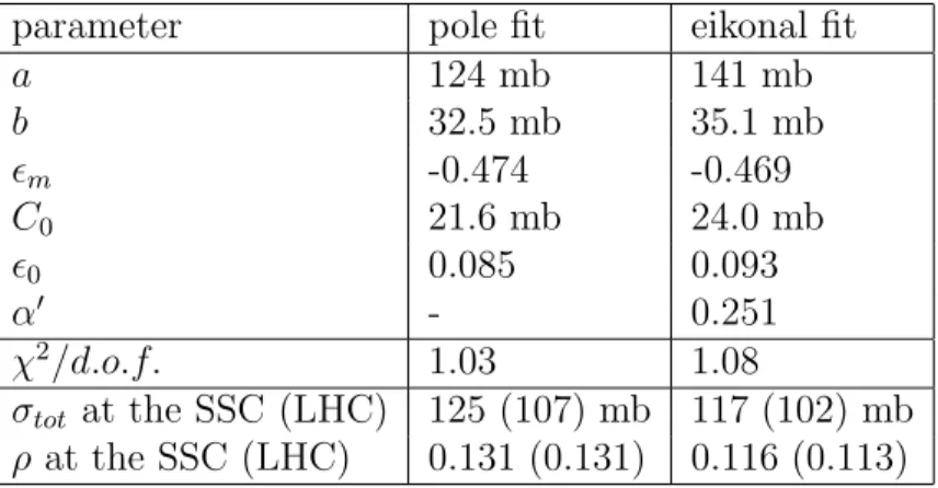
The most economical fit, inspired by Regge theory, is a sum of two simple Regge poles: A(s, t) s = (a ± ib)s ǫm+α′mt+ C 0sǫ0+α ′t (1) with a, b, C0 constants independent of s. The phase of the amplitude is obtained
by the imposition of s to u crossing symmetry. The first term has a universal part (a) representing f and a2 exchange, and a part (b) changing sign between p and ¯p
scattering, which comes from ρ and ω exchange. The second term (C0) is responsible
for the rise in σtot and is referred to as the “soft pomeron”. Its only obvious problem is
the eventual violation of the Froissart bound. Therefore, we also consider a unitarized version, for which we eikonalize the second term of Equation (1).
We give the best fit values of the parameters and the χ2/d.o.f. in Table 1.
parameter pole fit eikonal fit
a 124 mb 141 mb b 32.5 mb 35.1 mb ǫm -0.474 -0.469 C0 21.6 mb 24.0 mb ǫ0 0.085 0.093 α′ - 0.251 χ2/d.o.f. 1.03 1.08 σtot at the SSC (LHC) 125 (107) mb 117 (102) mb ρ at the SSC (LHC) 0.131 (0.131) 0.116 (0.113)
Table 1: Values of the parameters of Equation (1) that result from a least-χ2 fit to
data at t = 0.
The pole fit is shown by the lower curve of Figure 1 and the eikonalized one by the lowest curve of Figure 2. Both fits reproduce the data [9], from√s = 10 Gev to 1800 GeV with χ2/d.o.f. very close to 1. The only failure is the UA4 value for ρ, which is not
reproduced by most models, and for which further experimental confirmation seems to be needed. It is a curious fact that the eikonalized fit chooses the conventional value of the pomeron slope α′ which is normally derived from other constraints[6]. Also,
notice that unitarization does not make a big difference, and that even at the SSC, the difference between the two fits is only 8 mb.
Other parametrizations are possible, e.g. [7,8], and as shown by the proponents of this one [6], multiple Regge exchanges are essential to describe the data at nonzero t. However, as we limit ourselves here to the zero momentum transfer case for which the corrections are small, and as this simple form is particularly well suited for our purpose, we shall adopt it in the following as a starting point for the QCD evolution.
3
Theory: the hard pomeron
In order to describe total cross sections within the context of perturbative QCD, one can try, for s → ∞, to isolate the leading contributions and to resum them. This is made possible by the fact that perturbative QCD is infrared finite in the leading log s approximation and in the colour-singlet channel. This suggests that very small momenta might not matter, and that one could use perturbation theory.
Such a program has been developed by BFKL [3]. In a nutshell, one can show that, when considering gluon diagrams only, the amplitude is a sum of terms Tn of order
(log s)n and that terms of order (log s)n are related to terms of order (log s)n−1 by an
integral operator that does not depend on n, and that we shall write ˆK: Tn+1(s, kT2) = ˆKTn(s′, k′2T) = 3αS π k 2 T Z s s0 ds′ s′ Z dk′2 T k′2 T [Tn(s ′, k′2 T) − Tn(s′, kT2) |k2 T − kT′2| + Tn(s ′, k2 T) q k2 T + 4k′2T ]. (2)
This leads to:
T∞=X
n
Tn= T0+ ˆKT∞ (3)
This is the BFKL equation at t = 0. Its extension to nonzero t is known, but too complicated to handle analytically. We limit ourselves here to the zero momentum transfer case.
In this regime, the BFKL equation (3) possesses two classes of solutions. First of all, at fixed αS, the resummed amplitude is a Regge cut instead of a simple pole:
T∞≈R
dνsN(ν), with a leading behaviour given by
Nmax= 1 +
12 log 2
π αS (4)
Even for a small αS, say of order of 0.2, this leads to a big intercept Nmax ≈ 1.5. As
this is much too big to accomodate the data, and as a cut rather than a pole leads to problems with quark counting, subleading terms were added via the running of the coupling constant. It was first claimed that such terms would discretize the cut and turn it into a series of poles [10], but further work has shown that the cut structure remains [5,11]. However, the leading singularity is slightly reduced, and one can derive the bound [12]
Nmax > 1 +
3.6
Again, for values of αS of the order of 0.2, this leads to an intercept of the order of
1.23.
So, we reach a contradiction: on the one hand, the data demands that the am-plitude rises more slowly than s1+ǫ0, with ǫ
0 < 0.1; on the other hand, perturbative
resummation leads to a power s1+ǫp, with ǫ
p > 0.23. The difference between the two
is a factor 3 in the total cross section at the Tevatron. The resolution of this problem is far from clear, and one can envisage the implementation of some non-perturbative effects within the BFKL equation [5]. Rather than trying to understand ǫ0, we shall
here take a much simpler approach, i.e. assume a low-kT, low-s behaviour consistent
with the data, and see what general features its perturbative evolution might exhibit. The idea is to cut off Equation (3) by imposing k2
T > Q20, with Q0 big enough for
perturbation theory to apply, so that one uses the perturbative resummation only at short distances. Furthermore, one takes T0 ∼ s1+ǫ0 as the non-perturbative driving
term, valid for k2
T < Q20. This cut-off equation has been recently solved by Collins
and Landshoff [4] in the case of deep inelastic scattering. Most of their results and approximations can be carried over to the hadron-hadron scattering case, and we shall give here the basic features of the solution in this case.
First of all, the hadronic amplitude can be thought of as the convolution of two form factors times a resummed QCD gluonic amplitude obeying a cut-off BFKL equation.
A(s, t) = Z √s Q0 dk1 V (k1) k4 1 Z √s Q0 dk2 V (k2) k4 2 T (k1, k2; s) (6)
k1 and k2 are the momenta entering the gluon ladder from either hadron, √s is the
total energy, the two form factors V (ki), i=1,2, represent the coupling of the proton
to the perturbative ladder via a non-perturbative exchange, and the 1/k4
i come from
the propagators of the external legs. T (k1, k2; s) will obey the BFKL equation both
for k1 and k2, and the two independent evolutions will be related by the driving term
T0 representing the 2-gluon exchange contribution and thus proportional to δ(k1 −
k2)s1+ǫ0
. The next terms Tn will be given by Equation (2) but cut off at small k:
Tn(kT, k2; s) = θ(√s > kT > Q0) ˆKTn−1(kT′ , k2; s′) (7)
Under these assumptions, and working at fixed αs, one can show that the amplitude
(6) conserves the structure found in [4]: A s = C0s ǫ0 + ∞ X n=1 Cn(s)sǫn(s) (8)
This solution reduces to the usual solution of the BFKL equation when s → ∞ and Q0 → 0. The coefficients Cn depend on the model assumed for the coupling V (k)
between the non-perturbative and the perturbative physics and their s dependence is a threshold effect coming from the integration in (6). Their only general property is that they are positive. On the other hand, the powers ǫn(s) are universal functions
4
Interplay between soft and hard QCD: a model
As the coefficients of the series (8) are model-dependent, we do not attempt to calculate them, but rather try to assess the constraints that present data place on them. We shall then be able to decide whether such perturbative effects could play a substantial role in soft physics at future colliders. As all the Cn are positive, the behaviour of the
series (8) will not be very different from that of its leading term, and so we truncate it. We also make an educated guess for the threshold function contained in C1(s). This
does not affect our results for the values of Q0 shown here. We finally impose crossing
symmetry to get the real part of the amplitude. This gives ˜ A s = C0s ǫ0 + [c1(1 − Q0 √ s) 2 θ(√ s − Q0)] sǫ1(s) (9)
A(s) = A(s) + ˜˜ A(se−iπ) (10)
with c1 a positive constant. To calculate ǫ1(s) we assume that Q0 is the scale of αS
and take ΛQCD = 200 MeV. Using the results of reference [4], we calculate the curves
of Figure 3, for various values of the cutoff Q0 and thus of αS. One sees that the
effective power is much smaller than its purely perturbative counterpart (4), e.g. for Q0=2 GeV, the usual estimate (4) gives ǫ=0.8, whereas a cut-off equation gives values
half as big at accessible energies.
Again, we consider both a pole fit and an eikonalized one. Note that the use of such an eikonal formalism [13] is not derived from QCD. In fact, the BFKL equation in principle sums multi-gluon ladders in the s and t channels, so that in the purely perturbative case the eikonal formalism is probably too na¨ıve. However, in this case, it can be thought of as an expansion in the number of form factors V (k1)V (k2). This is
definitely not included in the BFKL equation. We further add the meson trajectories of (1) to the amplitude (9), and proceed to fit the data.
The first obvious observation is that the extra perturbative terms do not help the fit: due to the positivity of the Cn, they cannot produce a bump in ρ that would
explain the UA4 measurement. So, one gets the best fit when the new QCD terms are actually turned off. We want to examine here what constraints are placed on them by present data, and so we proceed as follows: we choose two values of Q0, 2 and 10
GeV, where one could imagine to cut-off perturbative QCD. We then proceed to fit the data, for increasing values of c1, letting all other parameters free. When we reach
the 90% confidence letter (C.L.) as defined by our χ2/d.o.f., we have found the highest
perturbative contribution permissible. For Q0 = 2 GeV, this gives c1/C0 ≤ 6 × 10⁻⁴
for the pole fit, and 2 × 10⁻³ for the eikonal one. For Q
0 = 10 GeV, the corresponding
values are 8 × 10⁻³ and 11 × 10−3. We plot the resulting curves in Figures 1 and 2.
The parameters of the non-perturbative component are modified from those of Table 1 by a few percent only. The coupling C0 is increased a little while the power ǫ0
goes down. This maximizes the perturbative contribution, which is mainly constrained by the Tevatron measurement of the total cross section. One sees that the small
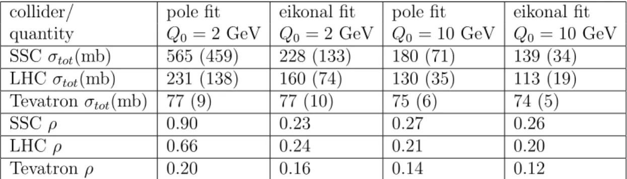
perturbative coupling can lead to quite dramatic consequences at the SSC and LHC. We show in Table 2 the 90% C.L. on the total cross section and the ρ parameter at future colliders. As the perturbative contribution can become very large, the effect of unitarization is non negligible, and depending on the value of Q0, the total cross
section could reach values as high as 230 mb at the SSC, with half of it coming from perturbative resummation.
collider/ pole fit eikonal fit pole fit eikonal fit
quantity Q0 = 2 GeV Q0 = 2 GeV Q0 = 10 GeV Q0 = 10 GeV
SSC σtot(mb) 565 (459) 228 (133) 180 (71) 139 (34) LHC σtot(mb) 231 (138) 160 (74) 130 (35) 113 (19) Tevatron σtot(mb) 77 (9) 77 (10) 75 (6) 74 (5) SSC ρ 0.90 0.23 0.27 0.26 LHC ρ 0.66 0.24 0.21 0.20 Tevatron ρ 0.20 0.16 0.14 0.12
Table 2: Allowed values of the cross section and the ρ parameter. The first two columns correspond to an infrared cutoff Q0 = 2 GeV and the two last ones to Q0 = 10 GeV,
see Equation (9). The number in parenthesis next to the cross section is the value of the perturbative component.
We emphasize that the estimates of Table 1 are conservative, as they correspond to cutoffs of 2 and 10 GeV. Cutting off the evolution when αS ≈ 1 would give a total
cross section of at least 3 b at the SSC, and be consistent with all available collider and fixed target data!
5
Conclusion
We have shown that the BFKL equation can be used to evolve the soft pomeron to higher s, and that perturbative effects could become measurable at the SSC/LHC. These effects are cutoff dependent, and perturbative physics seems to couple very weakly to the proton in the diffractive region, its coupling strength being a few percent of that of the soft pomeron. However, even a very weak coupling turning on at an energy of a few GeV can lead to measurable effects at sufficiently large energy. It is known that the pomeron couples to quarks, and quarks to gluons. Therefore, the coupling to the BFKL ladder cannot be zero, and specific models can be built for it [14].
This contribution is genuinely new and comes entirely from a QCD analysis. One should not be misled by previous parton models [8] which, while using a partonic picture, keep it mostly non-perturbative, replacing the small power sǫ0 of (1) by a small power x−ǫ0
in the gluon structure function xg(x). In the present model, xg(x) will contain the same powers ǫi(Q0/x) as the total cross section, but their coefficients
will in general be different from those entering the total cross section, and the relation between them will be model dependent.
The existence of such possibilities, and the fact that very large total cross sections are expected from the same kind of arguments that lead one to predict a rising cross section [13,15], shows that small momentum physics contains a wealth of open possibil-ities worth exploring experimentally. It also suggests that a large proportion of events could become calculable at very high energy, and so could be used for the detection of new physics.
Acknowledgments
References
[1] A. Bialas and P.V. Landshoff, Phys. Lett. B256, 540 (1991)
[2] J.D. Bjorken, preprint SLAC-PUB-5545 (May 1991), SLAC-PUB-5616 (March 1992)
[3] E.A. Kuraev, L.N. Lipatov and V.S. Fadin, Sov. Phys. JETP 44, 443 (1976) and 45, 199 (1977); Ya Ya Balitskii and L.N. Lipatov, Sov. J. Nucl. Phys. 28, 822 (1978)
[4] J.C. Collins and P.V. Landshoff, Phys. Lett. 276B, 196 (1992) [5] R.E. Hancock and D.A. Ross, preprint SHEP 91/92-14 (1992)
[6] A. Donnachie and P.V. Landshoff, Nucl. Phys. B267, 690 (1986); Nucl. Phys. B231, 189 (1984)
[7] C. Bourelly, J. Soffer and T.T. Wu, Mod. Phys. Lett. A6, 2973 (1991) [8] M.M. Block, F. Halzen and B. Margolis, Phys. Rev. D45, 839 (1992)
[9] E-710 Collab., presented at the International Conference on Elastic and Diffractive Scattering (4th Blois Workshop), Elba, Italy, May 22, 1991, to be published in Nucl. Phys. B (Proc. Suppl.) B25 (1992); CDF Collab., same proceedings; M. Bozzo et al., Phys. Lett. 147B, 392; M. Ambrosio et al., Phys. Lett. 115B, 495 (1982); N. Amos et al., Phys. Lett. 120B, 460 (1983); 128B, 343 (1984); U. Amaldi and K.R. Schubert, Nucl. Phys. B166, 301 (1980)
[10] L.N. Lipatov, Sov. Phys. JETP 63, 904 (1986); R. Kirschner and L.N. Lipatov, Zeit. Phys. C45, 477 (1990)
[11] G.J. Daniell and D.A. Ross, Phys. Lett. 224B, 166 (1989) [12] J.C. Collins and J. Kwiecinski, Nucl. Phys. B316, 307 (1989) [13] S. Frautschi and B. Margolis, Nuov. Cim. 57A, 427 (1968) [14] J.R. Cudell, work in progress.
[15] W. Heisenberg, in Kosmiche Strahlung (Springer-Verlag, Berlin:1953), p. 148; V. Gribov and A. Migdal, Sov. J. Nucl. Phys. 8, 583 (1969); N. W. Dean, Phys. Rev. 182, 1695 (1969); H. Cheng and T.T. Wu, Phys. Rev. Lett. 24, 1456 (1970); S.T. Sukhorukov and K.A. Ter-Martirosyan, Phys. Lett. 41B, 618 (1972)
Figure Captions
Figure 1: Pole fits (1) and (10) at zero momentum transfer, for pp (squares) and ¯pp (crosses) scattering. The lowest curve is the best (non-perturbative) fit, while the two upper curves are allowed by a cut-off BFKL equation at the 90% C.L., for an infrared cutoff Q0=2 GeV or 10 GeV, as indicated. (a) shows the total cross section and (b)
the ratio of the real-to-imaginary parts of the amplitude. The data are from reference [9].
Figure 2: Same as Figure 1, but after eikonalization.
Figure 3: The effective power of s of Equation (8) that results from a cut-off BFKL equation, for various values of the infrared cutoff Q0, as indicated next to the curves.