Green Function and Electromagnetic Potential for Computer Vision and Convolutional Neural Network Applications

(1)

UNIVERSITÉ DE MONTRÉAL

GREEN FUNCTION AND ELECTROMAGNETIC POTENTIAL FOR COMPUTER VISION AND CONVOLUTIONAL NEURAL NETWORK APPLICATIONS

DOMINIQUE BEAINI

DÉPARTEMENT DE GÉNIE MÉCANIQUE ÉCOLE POLYTECHNIQUE DE MONTRÉAL

THÈSE PRÉSENTÉE EN VUE DE L’OBTENTION DU DIPLÔME DE PHILOSOPHIAE DOCTOR

(GÉNIE MÉCANIQUE) JUIN 2019

(2)

UNIVERSITÉ DE MONTRÉAL

ÉCOLE POLYTECHNIQUE DE MONTRÉAL

Cette thèse est intitulée :

GREEN FUNCTION AND ELECTROMAGNETIC POTENTIAL FOR COMPUTER VISION AND CONVOLUTIONAL NEURAL NETWORK APPLICATIONS

présentée par : BEAINI Dominique

en vue de l’obtention du diplôme de : Philosophiæ Doctor a été dûment acceptée par le jury d’examen constitué de :

Mme CHERIET Farida, Ph. D., présidente

M. ACHICHE Sofiane, Ph. D., membre et directeur de recherche M. RAISON Maxime, Ph. D., membre et codirecteur de recherche M. PAMPLONA SEGUNDO Mauricio, D. Sc., membre

(3)

ACKNOWLEDGEMENTS

The first acknowledgment for my Ph.D. thesis goes to my directors Prof. Sofiane Achiche and Prof. Maxime Raison for their continued support, patience and motivation. They are both wise, knowledgeable, kind and helpful. It is hard to imagine going this far in my Ph.D. without their support, their open mind and their advice.

I would like to add a special thanks to the newest member of my family, my wife Nazanin Naderi, whom I married in the middle of my Ph.D. studies. Her continued kindness and support allowed me to outperform myself by starting each of my work days with happiness. She always pushed me to overcome every difficulty and never give up, and for that, I thank her immensely.

Other special thanks go to my parents for always being there for me and pushing me to overcome myself since my youth. My older sister Véronique for guiding me through life and providing me with an example of perseverance and kindness. My younger brother Rodrigue for being my lifelong rival and for his continued support at Polytechnique. I wish him good luck for his current Master’s degree and (maybe) his Ph.D.

I also acknowledge all of my co-workers for their support, their positive attitude and the great working environment that they provided. In truth, I considered each of my co-worker to be my friend, since they only provided joy and fun to the lab, and I hope they write their thesis soon! I would like to name Mahdis Asaadi, Olivier Brochu-Dufour, and Alexandre Duperré, who worked with me as highly dedicated interns. They helped me a lot in the progress of my Ph.D., but also taught me a lot from their own perspective and experience. I also want to thank Abolfazl Mohebbi for deciding to continue the project for industrial applications.

Another thank you goes to my friend and my favorite philosophy partner Fabrice Nonez. Although his true passion is pure mathematics, he was always there to help me have a deeper understanding of the applied mathematics that I was developing for my Ph.D.

Finally, I would like to thank all my friends and family for their continuous support. I can finally answer them when they ask me the everyday question, “when do you finish your Ph.D.?”

(4)

RÉSUMÉ

Pour les problèmes de vision machine (CV) avancées, tels que la classification, la segmentation de scènes et la détection d’objets salients, il est nécessaire d’extraire le plus de caractéristiques possibles des images. Un des outils les plus utilisés pour l’extraction de caractéristiques est l’utilisation d’un noyau de convolution, où chacun des noyaux est spécialisé pour l’extraction d’une caractéristique donnée. Ceci a mené au développement récent des réseaux de neurones convolutionnels (CNN) qui permet d’optimiser des milliers de noyaux à la fois, faisant du CNN la norme pour l’analyse d’images. Toutefois, une limitation importante du CNN est que les noyaux sont petits (généralement de taille 3x3 à 7x7), ce qui limite l’interaction longue-distance des caractéristiques. Une autre limitation est que la fusion des caractéristiques se fait par des additions pondérées et des opérations de mise en commun (moyennes et maximums locaux). En effet, ces opérations ne permettent pas de fusionner des caractéristiques du domaine spatial avec des caractéristiques puisque ces caractéristiques occupent des positions éloignées sur l’image.

L’objectif de cette thèse est de développer des nouveaux noyaux de convolutions basés sur l’électromagnétisme (EM) et les fonctions de Green (GF) pour être utilisés dans des applications de vision machine (CV) et dans des réseaux de neurones convolutionnels (CNN). Ces nouveaux noyaux sont au moins aussi grands que l’image. Ils évitent donc plusieurs des limitations des CNN standards puisqu’ils permettent l’interaction longue-distance entre les pixels de limages. De plus, ils permettent de fusionner les caractéristiques du domaine spatial avec les caractéristiques du domaine du gradient. Aussi, étant donné tout champ vectoriel, les nouveaux noyaux permettent de trouver le champ vectoriel conservatif le plus rapproché du champ initial, ce qui signifie que le nouveau champ devient lisse, irrotationnel et conservatif (intégrable par intégrale curviligne). Pour répondre à cet objectif, nous avons d’abord développé des noyaux convolutionnels symétriques et asymétriques basés sur les propriétés des EM et des GF et résultant en des noyaux qui sont invariants en résolution et en rotation. Ensuite, nous avons développé la première méthode qui permet de déterminer la probabilité d’inclusion dans des contours partiels, permettant donc d’extrapoler des contours fins en des régions continues couvrant l’espace 2D. De plus, la présente thèse démontre que les noyaux basés sur les GF sont les solveurs optimaux du gradient et du Laplacien. De ce fait, même s’il n’existe pas de solution exacte au gradient et au Laplacien, les

(5)

noyaux développés trouvent la solution la plus rapprochée possible d’un résultat, et ce en étant au moins 3.2 fois plus rapide que toute autre méthode de la littérature.

Ainsi, en utilisant notre solveur de gradient, nous avons développé la première méthode qui permet de combiner directement des matrices de contours avec des matrices de salience. L’amélioration des matrices de salience est en moyenne 6.6 fois supérieure au plus proche compétiteur sur des bases de données sélectionnées. Ensuite, pour améliorer notre algorithme de salience, nous avons développé le modèle DSS-GIS qui combine les contours et à la salience directement à l’intérieur d’un CNN profond. Cette combinaison a permis d’améliorer la performance du CNN, de réduire le surapprentissage et de réduire le temps d’apprentissage, pour une augmentation de seulement 10% du temps d’exécution. En plus, la couche GIS a permis d’améliorer les performances du

F-measure de 3.9% dans le cas d’images bruitées et de 2.3% dans le cas d’images à faible

luminosité. Finalement, nous avons développé un premier prototype qui permet d’utiliser les GF à différentes profondeurs dans un réseau de classification de chiffres. Ce prototype fonctionne en transformant le champ vectoriel de caractéristiques en un champ conservatif. Les premiers résultats sont prometteurs, car ils montrent une réduction du temps d’entrainement d’un facteur 5.2, une réduction du bruit dans les courbes d’apprentissage et une réduction de 28% de l’erreur de classification.

La principale retombée scientifique de la présente thèse est la création d’une nouvelle catégorie d’opérations pouvant être utilisés dans les CNNs. Ces opérations basées sur les GF permettent aux CNN de combiner l’information du domaine de l’image avec l’information du domaine du gradient, ce qui diffèrent entièrement des autres catégories d’opérations, soit les noyaux de convolutions, la réduction de taille (pooling) et les fonctions d’activations. Les GF permettent au CNN d’avoir un champ réceptif illimité, et ce à tout emplacement dans le réseau. De plus, ils permettent de convertir en un champ conservatif tout champ d’informations contenus dans les CNN. Enfin, dans le but d’étendre la portée du travail, ces opérations ont été codées dans différents langages, soit Matlab, C++ (OpenCV) et Python (Tensorflow et Pytorch).

(6)

ABSTRACT

For advanced computer vision (CV) tasks such as classification, scene segmentation, and salient object detection, extracting features from images is mandatory. One of the most used tools for feature extraction is the convolutional kernel, with each kernel being specialized for specific feature detection. In recent years, the convolutional neural network (CNN) became the standard method of feature detection since it allowed to optimize thousands of kernels at the same time. However, a limitation of the CNN is that all the kernels are small (usually between 3x3 and 7x7), which limits the receptive field. Another limitation is that feature merging is done via weighted additions and pooling, which cannot be used to merge spatial-domain features with gradient-domain features since they are not located at the same pixel coordinate.

The objective of this thesis is to develop electromagnetic (EM) convolutions and Green’s functions (GF) convolutions to be used in Computer Vision and convolutional neural networks (CNN). These new kernels do not have the limitations of the standard CNN kernels since they allow an unlimited receptive field and interaction between any pixel in the image by using kernels bigger than the image. They allow merging spatial domain features with gradient domain features by integrating any vector field. Additionally, they can transform any vector field of features into its least-error conservative field, meaning that the field of features becomes smooth, irrotational and conservative (line-integrable).

At first, we developed different symmetrical and asymmetrical convolutional kernel based on EM and GF that are both resolution and rotation invariant. Then we developed the first method of determining the probability of being inside partial edges, which allow extrapolating thin edge features into the full 2D space. Furthermore, the current thesis proves that GF kernels are the least-error gradient and Laplacian solvers, and they are empirically demonstrated to be faster than the fastest competing method and easier to implement.

Consequently, using the fast gradient solver, we developed the first method that directly combines edges with saliency maps in the gradient domain, then solves the gradient to go back to the saliency domain. The improvement of the saliency maps over the F-measure is on average 6.6 times better than the nearest competing algorithm on a selected dataset. Then, to improve the saliency maps further, we developed the DSS-GIS model which combines edges with salient regions deep inside the network. This combination helped improve the performance and reduce the overfitting of the

(7)

model using a single GF-based kernel at the last layer of each branch. The added GIS layer allowed an average F-measure improvement of 3.9% for noisy images and 2.3% for low-light images with only 10ms of additional computation cost. Finally, we developed an early prototype that uses the GF convolution at different points inside a classification network for digit recognition. It acts by transforming the field of features into the nearest possible conservative field. Early results show that it helped reduce the training time by a factor 5, reduce the noise in the validation curve and reduce the testing error by 28%, without increasing the computational capacity of the network. The main outcome of the current thesis is the creation of GF-based operations, a novel category of operations that can be used to improve CNN’s. Standard operations used in CNN are the convolutions, the pooling and the activation functions. The GF-based operations do not fit in any of these categories as they offer completely novel properties, allowing the network to have an unlimited receptive field at any given layer, to operate in the gradient-domain and to convert its features into conservative and physically interpretable features. Furthermore, the GF-based operations were written into different languages: Matlab, C++ (OpenCV) and Python (Tensorflow and Pytorch); allowing to deliver the work to the computer vision and machine learning community.

(8)

LIST OF TABLES

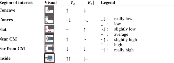
Table 3.1 : Potential and Field Characteristics at Different Regions of a Shape Filled with

Monopoles, for 𝑛 > 2 ... 26

Table 3.2 : Percentile Thresholds Used for the Discovery of the Regions of Interest ... 33

Table 3.3 : Qualitative Comparison Between Different Image Analysis Methods ... 42

Table 4.1 : List of fundamental properties for the consistency of the probabilities ... 58

Table 7.1 : Side layer information of HED and DSS architectures given by 𝑛, 𝑘 × 𝑘, where 𝑛 is the number of output channels and 𝑘 × 𝑘 is the size of the kernel. “Layer” is the name of the layer from the VGGnet-16 whose output is connected to a side layer. “1”, “2” and “3” represent the 3 layers for each side output. “1” and “2” are followed by a ReLU operation. If a GIS layer is added, 𝑛𝑜 = 3, otherwise 𝑛𝑜 = 1. ... 134

Table 7.2 : Comparison between the percentage testing results of HED and our HED-GIS. The * means that a denseCRF layer is added at the output. The best value in each category is highlighted in bold (ignoring GIS*). The values are in percentages. ... 144

Table 7.3 : Comparison between the testing results of DSS and our DSS-GIS. The * means that a denseCRF layer is added at the output. The best value in each category is highlighted in bold (ignoring GIS*). The values are in percentages. ... 145

Table 7.4 : Comparison of the proposed DSS-GIS and HED-GIS approaches (grey rows) with other saliency algorithms proposed in the literature. The best result of each column is highlighted in bold. The values are in percentages. ... 146

Table 7.5 : Comparison of the DSS and HED approaches with and without the proposed GIS layer when a 30% salt-and-pepper noise is added to the test set. The best result of each column is highlighted in bold. The values are in percentages. ... 148

Table 7.6 : Comparison of the DSS and HED approaches with and without the proposed GIS layer when a the brightness is reduced by 80% to simulate low-light pictures. The best result of each column is highlighted in bold. The values are in percentages. ... 149

Table 9.1 : Tools developed during the thesis in different languages and libraries ... 169

(15)

LIST OF FIGURES

Figure 1-1 : Overview of the objective and methodology of the thesis ... 3

Figure 2-1 : Example of saliency for a person image from the ECSSD dataset [68]; (a) Original image; (b) Ground-truth saliency map; (c) Saliency map produced by the DRFI method [67]; (d) Saliency map produced by the DSS method [26]. ... 11

Figure 2-2 : Image and channel sizes throughout the VGGnet-16 given by width × height × channels [10,83] ... 14

Figure 2-3 : Convolution kernel sizes given by width × height, number of neurons [10,83] ... 15

Figure 2-4 : Illustration of the InceptionNet v1 architecture, known as GoogLeNet [20,85]. ... 15

Figure 2-5 : Architecture of the ResNet neural network [84,85] ... 16

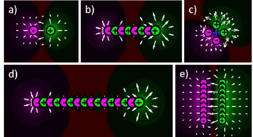
Figure 3-1 : Static electric potential and field of a: (a) positive monopole. (b) negative monopole ... 22

Figure 3-2 : Electric Potential and field for static monopoles placed as (a) a dipole. (b) a small chain of simple dipoles. (c) a horizontal and a vertical dipole, equivalent as 2 dipoles at 45°. (d) a long chain of simple dipoles. (e) simple dipoles in parallel. ... 23

Figure 3-3 : Potential and field with 𝑛 = 3 for positive monopoles placed on (a) A circle. (b) A corner. ... 25

Figure 3-4 : Example of convolution kernel for a particle potential matrix 𝑃𝑒 of size 7 × 7; (a) Euclidian distance from center 𝑟. (b) Potential of a centered monopole 𝑃𝑒 = 𝑉𝑒 , 𝑛 = 3 . ... 27

Figure 3-5 : Steps to calculate the normalized potential kernel for a dipole (a) Positive and negative monopoles at 1 pixel distance. (b) Potential kernel 𝑃𝑒 . (c) Dipole potential kernel 𝑃𝑑𝑖𝑝𝑥 resulting from the convolution of image “a” with kernel “b”. ... 28

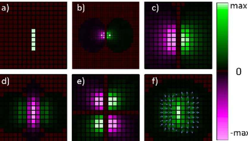
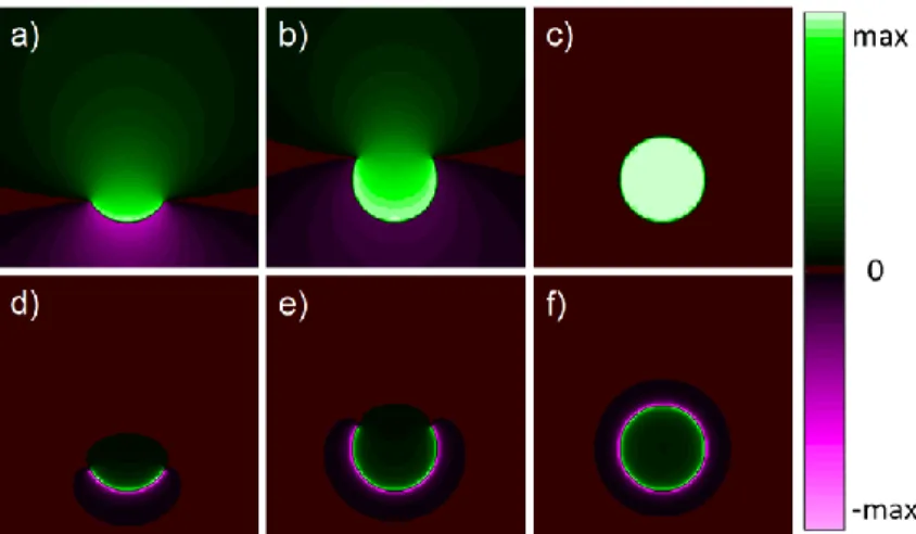
Figure 3-6 : Calculation of the potential and field of an image (a) Monopoles in the image. (b) Potential kernel 𝑃𝑒 . (c) Total potential 𝑉𝑒 . (d) Horizontal field 𝐸𝑒𝑥. (e) Vertical field 𝐸𝑒𝑦 . (f) Field norm 𝑬𝑒 and direction ... 29

(16)

Figure 3-7 : Steps to calculate the magnetic PF of an image (a) Dipoles in the image. (b) Horizontal dipole potential kernel 𝑃𝑚𝑥 . (c) Total potential 𝑉𝑚 . (d) Horizontal field 𝐸𝑚𝑥. (e) Vertical field 𝐸𝑚𝑦 . (f) Field norm 𝑬𝑚 and direction. ... 30 Figure 3-8 : (a) Special shape with the white region being a uniform density of charge, used to

compute the following PF with 𝑛 = 3. (b) The potential 𝑉𝑒. (c) The field 𝑬𝑒. (d) The potential squared only on the contour 𝑉𝑒onC2. (e) The field squared only on the contour 𝑬𝑒onC2. .. 32 Figure 3-9 : RoI found on a complex shape using a contour analysis by potential and field

thresholds. (a) Concave regions. (b) Convex regions. (c) Flat regions. (d) Regions near the CM. (e) Regions far from the CM. (f) Regions inside the shape. ... 33 Figure 3-10 : RoI found on a complex shape (filtered with a twirl, twist and wave distortion) using

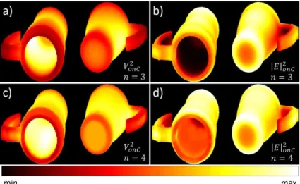
a contour analysis by potential and field thresholds. (a) Concave regions. (b) Convex regions. (c) Flat regions. (d) Regions near the CM. (e) Regions far from the CM. (f) Regions inside the shape. ... 34 Figure 3-11 : EM potential 𝑉 and field 𝐸 generated by a 3D mug, with different values of 𝑛. (a)

𝑉𝑜𝑛𝐶2 with 𝑛 = 3. (b) 𝐸𝑜𝑛𝐶2 with 𝑛 = 3. (c) 𝑉𝑜𝑛𝐶2 with 𝑛 = 4. (d) 𝐸𝑜𝑛𝐶2 with 𝑛 = 4. ... 35 Figure 3-12 : Potential 𝑉𝑚 resulting of the convolution of a dipole perpendicular to the partial

contour lines. (a) Partial contour with low resolution 64x64. (b) Dipole with 𝑛 = 3 and low resolution. (c) Dipole with 𝑛 = 2 and low resolution. (d) Partial contour with high resolution 512x512. (e) Dipole with 𝑛 = 3 and high resolution. (f) Dipole with 𝑛 = 2 and high resolution. ... 36 Figure 3-13 : Potential 𝑉𝑚 of a circular partial contour magnetized perpendicular to their

orientations. (a) Circle arc of 90°, with 𝑛 = 2. (b) Circle arc of 270°, with 𝑛 = 2. (c) Circle arc of 360°, with 𝑛 = 2. (d) Circle arc of 90°, with 𝑛 = 3. (e) Circle arc of 270°, with 𝑛 = 3. (f) Circle arc of 360°, with 𝑛 = 3. ... 37 Figure 3-14 : PF computed from the initial partial contour, with 𝑛 = 2 and the dipole perpendicular

to the partial contours. (a) Initial partial contour. (b) Potential of attraction 𝑉𝑚. (c) Potential of repulsion 𝑉𝑚. (d) Field of attraction 𝐸𝑚0.5. (e) Field of repulsion 𝐸𝑚0.5. ... 38

(17)

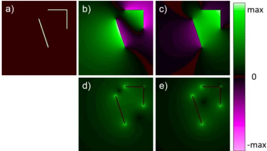
Figure 3-15 : Partial contours for the number “2” at the left, with the potentials 𝑉𝑚 of dipoles perpendicular to the partial contours, with 𝑛 = 2. (a) Clean partial contour. (b) Deformed partial contour. (c) Heavily distorted partial contour. ... 39 Figure 3-16 : Contour approximation via Fourier descriptors. (a) Fourier descriptor with 4

harmonics. (b) Fourier descriptors with 32 harmonics. [37,38] ... 43 Figure 4-1 : Definitions of different concepts. (a) Image of an elk from BSD500 dataset. (b) Edges

computed using the Sobel algorithm. (c) The contour of the elk. (d) Partial contour (stroke) along with 2 possible paths that close the partial contour. ... 47 Figure 4-2 : Example of a partial contour 𝑆 between points 𝛾𝑖, 𝑓, closed by a path 𝑆𝑛 to generate

the region 𝑅𝑛 containing the point 𝛾𝑖𝑛 but excluding 𝛾𝑜𝑢𝑡. 𝑆 is an existing partial contour and does not have restrictions. 𝑆𝑛 is the generated path used to close 𝑆, thus 𝑆𝑛 must be non-self-intersecting, convex and smooth. ... 50 Figure 4-3 : Example of 7 paths 𝑆𝑛 between points 𝛾𝑖 and 𝛾𝑓, with starting angles 𝛽1 → 5 + and

𝛽1 → 2 −, such that 𝑅𝑛, the region between 𝑆𝑛 and 𝑆, is a subset of 𝑅𝑛 + 1 ... 51 Figure 4-4 : Example of a circular path between points 𝛾𝑖 and 𝛾𝑓, with a starting angle 𝛽 ... 53 Figure 4-5 : Example of 2 regions 𝑅(𝛽1,2+) formed by the closure of the path 𝑆 with the circular

arcs 𝑆𝐶𝛽1,2 + ... 53 Figure 4-6 : Example of (a) a partial contour 𝑆 that intersect a circular arc 𝑆𝐶 at the point 𝛾 ×. (b)

The region inside the closure of the partial contour 𝑆 with the sub-paths 𝑆𝐶 − and 𝑆𝐶 +. .. 54 Figure 4-7 : Example of (a) A complex intersection between 𝑆 and 𝑆𝐶. (b) The regions that do not

respect the logical operation are eliminated. (c) The region 𝑅 is formed with a union of the remaining regions. ... 55 Figure 4-8 : Complementarity of the enclosure probability across the path 𝑆. (a) 2 points at an

opposed side of 𝑆. (b) Multiple complementary points, at opposed sides of 𝑆, but with an infinitesimal distance. ... 57 Figure 4-9 : A line on the 𝑥 axis, composed of dipoles parallel to the 𝑦 axis. ... 59

(18)

Figure 4-10 : Example of equipotential lines of 𝑉𝑚 (green and pink) computed on 6 different partial contours (dark grey), with the light grey lines being the perfectly circular equipotential lines of equations (40) and (41) ... 62 Figure 4-11 : Algorithm used for repulsion optimization by flipping the magnetic orientation of

each individual or group of sub-partial contours 𝐺𝑘. ... 64 Figure 4-12 : (a) Artificial image composed of different nearby shapes (b) Extracted partial

contours using Canny [63]; (c) Resulting 𝑉𝑚 in the initial orientation; (d) resulting 𝑉𝑚 after the repulsion optimization. ... 64 Figure 4-13 : (a) Artificial image composed of different adjacent shapes (b) Extracted partial

contours using Canny [63], with the double boundaries in green; (c) Resulting 𝑉𝑚 without the double boundary; (d) resulting 𝑉𝑚 with the double boundary. ... 65 Figure 4-14 : The algorithm used for the image splitting into multiple sub-images ... 66 Figure 4-15 : Example of image splitting process; (a, b, e) The temporary states of the splitting; (c,

d, f, g) The final set of split potentials 𝑣𝑚𝑖... 67 Figure 4-16 : Comparison of the original images with the probabilistic reconstruction. (a, c, e)

Original synthetic image composed of different shapes with the partial contours (orange); (b, d, f) Probabilistic weighted reconstruction based on the partial contours (orange). ... 72 Figure 5-1 : Process summary of the gradient domain image editing. ... 86 Figure 5-2 : Computation time (ms) in logarithmic scale for a single channel gradient solving of

resolution of 801x1200, including the preparation time. The Perez [57] and Tanaka [61] methods have no GPU implementation. The Pytorch* implementation is tested on batches of 100 images, and the total time is divided by 100. ... 90 Figure 5-3 : Comparison of the RMSE between 𝑬𝑐 and 𝑬𝑝, where the thresholds are the

perturbation used to generate 𝑬𝑝. The displayed values are the mean of the RMSE on the 1000 images of the ECSSD dataset [68]. ... 91 Figure 5-4 : Example of Poisson Blending application; (a) Stamp to copy, with the red-dotted lines

(19)

accidentally cropped; (b) destination image; (c) Poisson blending from Perez algorithm [57,118]; (d) Proposed GFC blending. ... 92 Figure 5-5 : Example of gradient thresholding and solver steps. (a) Original image; (b) Gradient 𝑬;

(c) Thresholded gradient at 10%; (d) Solved image 𝐼𝑐, 𝑐𝑜𝑟𝑟. ... 93 Figure 5-6 : Examples of solved images 𝐼𝑐, 𝑐𝑜𝑟𝑟 after the gradient threshold at 10%. (a) Image of

a castle; (b) Solved castle image after 10% gradient threshold; (c) Image of a leopard; (d) Solved leopard image after 10% gradient threshold. ... 94 Figure 5-7 : Examples of the steps involving the GDM equation (73). (a) Original image; (b)

𝑬: Gradient; (c) 𝑬𝑝: Gradient merged with the SE method [64] and 𝛼 = 0.5; (d) Solved image. ... 95 Figure 5-8 : Example of GDM using equation (73) with a random forest edge detector [64] and

varying parameter 𝛼. ... 96 Figure 5-9 : Examples of solved images 𝐼𝑐, 𝑐𝑜𝑟𝑟 with a perturbed gradient from equation (73) with

edges information from SE method [64] and RCF method [25] and 𝛼 = 0.5. ... 97 Figure 5-10 : Comparison of edge merging methods. (a) Original image; (b) Saliency sharpening

from Bhat et al. [58]; (c) Enhancement using our GDM method with 𝛼 = 0.5 and SE edge detector. ... 97 Figure 5-11 : Examples of solved images 𝐼𝑐, 𝑐𝑜𝑟𝑟 with a perturbed gradient from equation (73)

with edges information from SE method [64] with NMS and 𝛼 = 0.5. ... 99 Figure 6-1 : Diagram of the complete SEE method, which allows improving the saliency via a

combined image preprocessing and saliency map postprocessing. The images are examples of the results at each step based on the DRFI method with a precision/recall curve for the selected example where 𝑆𝐼 is the original saliency and 𝑆𝐼0𝑅𝑅𝐶 is the same saliency improved using our SEE method. ... 104 Figure 6-2 : Comparison of SE and RCF edge detection methods trained or finetuned on the

BSDS500 or MSRA10K datasets, with the number of iterations of retraining, using 2 example images from the ECSSD dataset. The salient edges will be used as inputs for the proposed SEE method. ... 105

(20)

Figure 6-3 : Diagram of the core GDM function, allowing to merge image/saliency information with edges information by passing to the gradient domain and solving the Laplacian equation to go back to the image domain. ... 109 Figure 6-4 : Diagram of the SEE-Post method, which allows to post-process a saliency map based

on the salient edge detection. The images are examples of the results at each step based on the DRFI method with a precision/recall curve for the selected example. ... 110 Figure 6-5 : Diagram of the SEE-Pre method, which allows preprocessing an image based on the

salient edge detection for a more accurate saliency map. The images are examples of the results at each step based on the DRFI method with a precision/recall curve for the selected example. ... 113 Figure 6-6 : Smooth-step function (85) with different values of 𝐾. ... 115 Figure 6-7 : Comparison of the results from 5 different SoA methods (MC, RBD, DRFI, DCL, and

DSS) and their improvement using our SEE algorithm highlighted in green. The examples are chosen as some of the most difficult images in the datasets. ... 117 Figure 6-8 : Comparison between the regular saliency methods, the enhanced saliency using our

SEE-Post algorithm and the enhanced saliency using our SEE algorithm. A higher percentage is better for 𝐴𝑈𝐶, 𝐹𝑚, 𝑃𝑅 and 𝑃max , but a lower percentage is better for 𝑀𝐴𝐸. The 3 datasets used are ECSSD (E), PASCAL-S (P-S) and DUT-OMRON (D-O). ... 120 Figure 6-9 : Precision-recall curves comparing 6 different methods (DSR, RBD, DRFI, MC, DCL,

and DSS) with and without our SEE method on 3 different datasets. ... 121 Figure 6-10 : Comparison of the improvement over 𝐹𝑚 and 𝑀𝐴𝐸 for different SoA saliency

improvement methods. ... 122 Figure 7-1 : Graph summary of the gradient integration and sum (GIS) layer, which outputs 𝑛

channels from 3𝑛 inputs. ... 130 Figure 7-2 : The HED [66] and DSS [11,26] architectures nested upon the pre-trained VGGnet-16

[10] network, with a total of 6 side layers. The red arrows are the short connections implemented by the DSS model [11,26]. Our contribution is the GIS at the end of each side-layer, which requires the layer sideX_3 to output 3 channels instead of 1. ... 132

(21)

Figure 7-3 : Closer view on the integration of the GIS layer inside the DSS architecture. For the HED architecture, the GIS layer is placed directly after the channel split since there are no short connections. ... 133 Figure 7-4 : Example of the inputs of the GIS layer coming from a fully trained HED-GIS network.

𝑆 is expected to be in the saliency domain; 𝐸𝑥, 𝐸𝑦 are expected to represent the 2 components of the gradient domain. ... 135 Figure 7-5 : Test results comparison between the DSS and HED methods with and without the

proposed GIS layer. ... 141 Figure 7-6 : Comparison of the validation curves of different models for the optimally found

parameters. The validation performance is computed every 500 iterations on the full validation set. ... 142 Figure 7-7 : Comparison of 6 validation curves in orange of our implementation of the DSS model,

and 6 validation curves in blue of our DSS-GIS model. The curves are smoothed using exponential smoothing with a factor 0.9, and the x-axis represents the number of iterations. ... 142 Figure 7-8 : Precision-Recall curves (top row) and true-positive/false-positive curves (bottom row)

for the 3 test datasets ... 146 Figure 7-9 : Test results comparison between the DSS and HED methods with and without the

proposed GIS layer, when the test set is modified with noise or reduced brightness. ... 148 Figure 7-10 : Performance impact of adding noise to the testing set for the DSS and the proposed

DSS-GIS methods. ... 149 Figure 8-1 : Inception module of the Google-net [20] with an added GDI2 or GDI3 layer. The

Conv + R indicate a convolutional layer with a Relu activation function, the 𝑛 × 𝑛 means that the kernel size is 𝑛 and the 𝑚S means that the stride is 𝑚. ... 153 Figure 8-2 : Internal structure of the GDI2 which splits the data into 2 inputs for the GFC; and

GDI3 which splits the data into 3 inputs for the GDM or GIS layers. The 𝑑𝑥 and 𝑑𝑦 represent numerical derivatives and the Conv-layer does not use an activation function or bias; the 𝑛 × 𝑛 means that the kernel size is 𝑛 and the 𝑚S means that the stride is 𝑚. ... 154

(22)

Figure 8-3 : Validation accuracy on the MNIST dataset for a smaller Google-net with 2 inception layers. The blue line is the standard network and the orange line is the same network with the added GID2 in each inception layer. ... 155 Figure 9-1 : Example of saliency maps produced with a single layer of convolution network which

is able to perfectly detect the salient edges, but not the regions within the edges. The images are not real results, they are produced by an image editing software. (a1) Original image; (a2) True saliency value; (b1) Detected normalized saliency features with the small receptive field; (b2) Final saliency after thresholding; (c1) Detected normalized directional gradient of saliency features with the small receptive field; (c2) extended features using the GFC; (c3) Final saliency after GFC and thresholding. ... 163 Figure 9-2 : Example of documentation used for our green_function_torch module. ... 170 Figure 9-3 Our contribution, in terms of categories of possible operations inside CNN. ... 172 Figure 10-1 : Neural network architecture with the neurons being the yellow circles, with a view

inside the neurons ... 190 Figure 10-2 : Static electric potential and field of a: (a) positive monopole. (b) negative monopole ... 192 Figure 10-3 : Electric Potential and field for static monopoles placed as (a) A simple dipole. (b) A

small chain of simple dipoles. (c) A horizontal and a vertical dipole, equivalent as 2 dipoles at 45°. (d) A long chain of simple dipoles in series. (e) A long chain of simple dipoles in parallel. ... 193 Figure 10-4 : Potential and field for circles, with 𝑛 = 3, for (a) positive monopoles. (b) parallel

dipoles. The green part is the positive charges/potential, and the purple part is the negative charges/potential. ... 196 Figure 10-5 : Potential and field for corners of (a) positive monopoles. (b) parallel dipoles. ... 197 Figure 10-6 : Example of different symmetric paths between points 𝛾𝑖 and 𝛾𝑓, with a starting angle

𝛽 ... 201 Figure 10-7 : Example of a circular path between points 𝛾𝑖 and 𝛾𝑓, with a starting angle 𝛽 ... 204 Figure 10-8 : Demonstration that the potential 𝑉𝑚 has circular equipotentials ... 206

(23)

LIST OF SYMBOLS AND ABBREVIATIONS

The list of symbols and abbreviations presents the symbols and abbreviations used in the thesis or dissertation in alphabetical order, along with their meanings. First, we present the list of symbols, then the list of abbreviations.

Latin symbols

𝐶, 𝐶₀ Edge intensity computed from an edge detection method

𝑑𝑖𝑝 Dipole

𝑒, 𝑚 Electric (𝑒) or Magnetic (𝑚)

𝑬_𝑒,𝑚 Virtual Vector field associated to electric 𝑒 or magnetic 𝑚 charge 𝑬 Electric field, being the gradient of 𝑉_𝐸 or 𝑉_𝑚

𝑬_𝑐 Reconstructed conservative electric field 𝑬𝑝 Perturbed non-conservative electric field

𝐹 Density correction factor of 𝐼 𝐹_𝑚 F-measure on a given dataset 𝐺 Binary ground truth of the saliency 𝐺_𝑘 A possible group of different 𝑠_𝑖 or 𝑆

𝐼 Image matrix, with values between -1 and +1 𝐼0 Input image normalized in the range [0, 1]

𝐼_𝑅 The resulting image after solving the Laplacian 𝐿_𝑝

K_I→E Complex kernel used to compute the gradient 𝑬 from an image 𝐼₀ KE→L Complex kernel used to compute the Laplacian 𝐿𝑝 from a gradient 𝑬

𝐾_𝛻2 Convolution kernel for the Laplacian operator 𝐾̌_𝛻2 Zero-padded Laplacian kernel

(24)

𝐾_𝜃 Complex derivative kernel in 2D 𝐿_𝑝 Laplacian of the image 𝐼₀

𝑀 Binary mask generated by a threshold on 𝑆

𝑀𝐸 Function used to merge the norm of the gradient with the edges

𝑀_𝜃 Function used to merge the orientation of the gradient with the edges 𝑁 Number of partial contours, or Total number of pixels in an image

𝑛 Number of spatial dimensions for the virtual potential (𝑛 = 2 for an image) 𝑜𝑛𝐶 Only values on the Contour

𝑃 Precision of 𝑆 against 𝐺 𝑃_max Maximum value of 𝑃

𝑃_{𝑒,𝑚,𝑑𝑖𝑝} Virtual Potential kernel of a monopole or dipole 𝑃𝑒 Electric potential by a single monopole

𝑃_𝑑𝑖𝑝𝜃 Complex dipole potential

𝑃𝑆 Probability of being enclosed in 𝑆

𝑃_𝑆± The value of 𝑃_𝑆 associated to 𝑉_𝑚±

PR

̅̅̅̅ Average of the precision-recall curve 𝑃𝐼0→1 Preparation step for the image 𝑃_𝐶_0→1 Preparation step for the edges 𝑞_𝑒,𝑚 Virtual Charge

𝑟 Euclidean distance

𝑅 The region inside a closed 𝑆, or Recall of 𝑆 against 𝐺

𝑆 Partial contour, defined as a partial contour, or Saliency map defined in the range [0, 1]

(25)

𝑆_𝐶± The sections of 𝑆_𝐶 defined with 𝛽±

𝑆𝑛 The n-sphere area constant (𝑆2 = 2𝜋)

𝑠_𝑖 A part of the partial contour 𝑆 𝑡 Time for parametric functions 𝑡𝑖,𝑓 Initial and final time

𝑈 Any possible potential, meaning that ∆𝑈 is any possible field 𝑉_𝑒,𝑚 Virtual Potential associated to electric 𝑒 or magnetic 𝑚 charge 𝑉𝑚± Region where the 𝑉𝑚 is expected to be positive/negative

𝑉_𝐸 Potential, often represents the signal or computed image 𝑉_{𝐸,𝑐𝑜𝑟𝑟} Potential corrected to preserve colours and contrast

𝑉mono Green’s function, equivalent to electric potential by a single monopole

𝑉_monoℱ _{Optimal Green’s function in the Fourier domain}

𝑽dip Gradient of 𝑉mono

𝑉_dip𝜃 Complex dipole potential 𝑊𝑆 Weighted probability

𝑤_𝑆 Weighted probability of a sub-image 𝑥_𝑚 Cartesian coordinate in the dimension 𝑚 𝑥, 𝑦 Horizontal and vertical axis

Greek or scripts symbols

𝛼 Factor between 0 and 1 to preserve the edge invariance

𝛽 The starting angle of a symmetric 𝑆, or parameter of the F-measure set to 0.3 𝛽± The starting angle from one side of 𝑆, or the other side

(26)

𝛿̌ Zero-padded numerical Dirac’s delta

𝜃 Orientation matrix perpendicular to the partial contours in 𝐼 𝜃𝐶 Orientation of the edges 𝐶

𝜃_𝐸 Orientation of the gradient 𝑬 𝛾 A specific point in space

𝛾𝑖,𝑓 The starting and ending points of 𝑆

𝓔𝑒,𝑚 Electromagnetic vector field according to physics [V m−1]𝑒, [V s m−2]𝑚

𝓥_𝑒,𝑚 Electromagnetic potential according to physics [V]_𝑒, [V s m−1]_𝑚

ℱ Fourier transform

ℱ−1 Inverse Fourier transform

ℜ(), ℑ() Real part ℛ or Imaginary part ℐ of any complex value

𝜎 Standard deviation

Ω(𝑓) Variance of 𝑓

Operators

∆𝑥,𝑦 Numerical derivative kernel in 𝑥̂ or 𝑦̂ direction

∇ Gradient operator

∇2 _{Laplacian operator}

∇ ⋅ Divergence operator

⋅ Scalar product

∗ Convolution operator

∘ Hadamard product (Element-wise multiplication) ⊂ Subset operator, used to indicate 𝛾 is inside 𝑅 ∩ Intersection (AND operator)

(27)

∪ Union (OR operator) ⋃ 𝑎𝑖 𝑖 Union of all the elements 𝑎𝑖

±? Either sum or subtraction, to be decided

̅ Mean value

! _{Logical NOT operator}

Abbreviations

AUC Area under the true-false-positive curve

CAMERA-I Convolutional approach of magnetic and electric repulsion to analyse an image CNN Convolutional neural network

CPU Central processing unit

CV Computer vision

DSS-GIS Deeply supervised saliency with gradient integration and sum EM Electromagnetic OR Electromagnetism

FFT Fast Fourier transform

GDIE Gradient domain image editing GDM Gradient-domain merging GIS Gradient integration and sum

GF Green’s function

GFC Green function convolution GPU Graphic processing unit MAE Mean absolute error between

NN Neural network

PIIPE Probability of inclusion inside partial edges Post For postprocessing

(28)

Pre For preprocessing RGB Red green blue

RMSE Root-mean-squared-error

SEE Saliency enhancement using edges SoA State of the art

(29)

LIST OF APPENDICES

APPENDIX A BENCHMARKING PARAMETERS ... 187 APPENDIX B STANDARD NEURAL NETWORKS ... 189 APPENDIX C GENERAL ELECTROMAGNETISM ... 191 C.1 Supplementary Nomenclature ... 191 C.2 Monopoles and Dipoles ... 191 C.2.1 Electric monopoles ... 191 C.2.2 Electric dipoles ... 192 C.2.3 Magnetic charges and dipoles ... 193 C.3 Mathematical Laws of EM ... 194 C.3.1 Maxwell’s Equations ... 194 C.3.2 Adaptation of Maxwell’s equations for Computer Vision ... 195 C.4 Geometrical Interpretation of Maxwell’s Equations ... 196 C.4.1 Closed shapes with particles on the contour ... 196 C.4.2 Corners with particles on the contour ... 197 C.5 Partial contour Manipulations ... 197 C.5.1 Grow and unite contour regions ... 198 C.5.2 Finding Partial contour Orientation ... 199 APPENDIX D GENERAL ELECTROMAGNETISM ... 201

D.1 Supplementary nomenclature ... 201 D.2 Paths characteristics ... 201 D.2.1 Characteristics of the paths between 2 points ... 201 D.2.2 Choosing the circle, rejecting the parabola ... 202 D.2.3 Circular path parameters ... 203

(30)

D.3 Electromagnetic potential ... 204 D.3.1 Elliptical potentials and paths ... 204 D.3.2 Convolution alternative ... 205 D.3.3 Demonstration that equipotential lines are circular ... 205

(31)

CHAPTER 1 INTRODUCTION

Since the year 2000, there has been an exponential rise in the sale of consumer digital cameras [1] followed by the bigger rise of smartphones equipped with digital cameras [2] and the exponential increase in the commercial robotics market [3]. Those factors led directly to an explosion in the computer vision (CV) and artificial intelligence (AI) market, both in robotics and in data analysis [4]. For example, our research lab uses CV to perform airplane topological optimization [5], intelligent robot control for the disabled using eye-tracking [6,7] and automated drone control. Then, the years 2010s have been revolutionary in terms of image understanding thanks to the rise of machine learning algorithms and convolutional neural networks (CNN). The CNN was initially able to outperform any standard algorithm for image classification purposes [8–10]. Then, they were used to solve the binary problems of CV, such as edge detection, skeleton extraction and saliency [11], and are now performing at near human level.

Chapter 1 In the field of machine learning and CV, many successful methods were based on the biological observation of nature. For example, the structure of the CNN is heavily inspired by the way the frontal cortex analyses images [9,12]. However, there are limited uses of physically inspired models. For example, the usage of electromagnetic (EM) based fields is limited to quadrupole text orientation [13] and the gravity-based edge detection [14]. Although those methods were inspired by a physical model and they initially performed well, they were soon outpaced by competing methods. One of the reasons is that they used the potentials and fields convolutions in an intuitive way such as bluring filters and derivative filters. The current thesis differs since it thoroughly studies the mathematical behavior of EM and GF for image convolutions.

1.1 Objectives

The main objective of the current thesis is to develop electromagnetic (EM) convolutions and Green’s functions (GF) convolutions to be used in Computer Vision and convolutional neural networks (CNN).

The main objective can be divided into the following sub-objectives (Obj):

Obj - 1. Develop a mathematical and intuitive understanding of the behavior of EM and GF convolutions in an image.

(32)

This objective allows to better guide the research decisions and to better understand the results. It was fundamental for the next sub-objectives.

Obj - 2. Use the GF convolutions to reduce the computation time and numerical error of the EM and allow fast and efficient gradient-domain image editing.

This objective allows editing an image in a non-intuitive way by enhancing or reducing the gradient of the image at specified locations.

Obj - 3. Use the GF to improve the results of CNN for salient object detection and digit classification.

This objective allows improving the extracted features by using the properties of conservation of energy and smoothness of EM. It also allows the current work to have a broader impact on the CV community since an important part of the research focuses of CNN.

1.2 Methodology

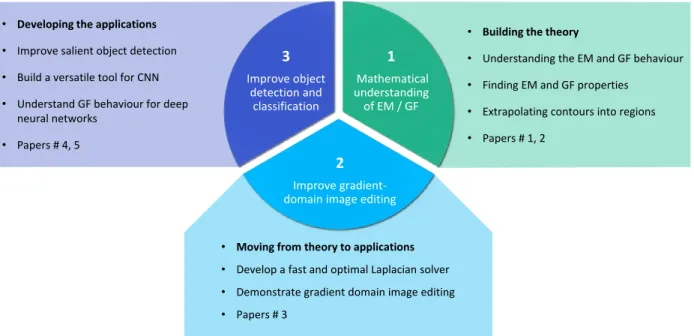
To answer the objectives given previously, a total of 5 papers were written and are included as chapters in the current thesis. This section will present a summary of the methodology and the articles developed to answer each of the sub-objectives. First, an overview of the objectives of the thesis is presented in Figure 1-1, followed by the detailed methodology below.

(33)

Figure 1-1 : Overview of the objective and methodology of the thesis

Obj - 1. The thesis first studies how Maxell’s equations of EM behave in an image using their numerous physical, geometrical and mathematical properties. The study is presented in our first paper [15] in Chapter 3. It computes the EM potential and field using numerical convolutions and performs a qualitative analysis of the results. Then, the second paper [16] presented in Chapter 4 demonstrates mathematically that dipole potentials can be used to compute the probability of belonging inside partial contours. For example, the paper showed how the resulting potential allows reconstructing the shapes when only incomplete contours are provided. These two papers were fundamental for answering the first objective, specifically to develop a mathematical and intuitive understanding of the behavior of EM convolutions in an image.

Obj - 2. After demonstrating the usefulness of EM potential and fields, the GF is developed in the paper [17] presented in Chapter 5. The GF reduces the numerical error to almost zero and improves the computation time by a factor 4 compared to EM. In fact, we have proven mathematically that, when a non-conservative perturbation is added to a gradient, the GF convolution (GFC) is the least-error gradient or Laplacian solver. Plus, it is shown to perform well on multiple tasks of gradient domain image editing. Hence, this paper answers the second objective of the current thesis, specifically to reduce the computation time and numerical error of the EM potentials while developing a gradient domain editing method.

• Building the theory

• Understanding the EM and GF behaviour • Finding EM and GF properties

• Extrapolating contours into regions • Papers # 1, 2

1

Mathematical understanding

of EM / GF

• Moving from theory to applications • Develop a fast and optimal Laplacian solver • Demonstrate gradient domain image editing • Papers # 3

2

Improve gradient-domain image editing

• Developing the applications • Improve salient object detection • Build a versatile tool for CNN • Understand GF behaviour for deep

neural networks • Papers # 4, 5 3 Improve object detection and classification

(34)

Obj - 3. Using the efficient GFC Laplacian solver, the current objective is to improve salient object detection and neural network using the gradient domain. At first, the objective focueses on salient object detection, with the paper [18] presented in Chapter 6. In this work, we developed a method that combines the output of a saliency network with the output of an edge detection network using a novel method we called gradient domain merging (GDM). The GDM uses the gradient domain to merge features of different nature (edges vs regions), then uses a GFC to solve the perturbed gradient. It showed to be fast and effective at improving the saliency maps of different methods. Then, the next paper [19] presented in Chapter 7 shows that another GFC-based operation, called gradient integration and sum, can be added inside different CNN to improve the testing saliency maps further, to reduce the training convergence time, to reduce the model overfitting and to increase the robustness against parameter initialization and noise. Finally, additional prototypes are developed in section 8.1 to demonstrate that GFC can be added within the Google-net [20] to improve its training time and testing performance on the MNIST dataset [8]. These 3 chapters and section allowed to answer the third objective of the current thesis, specifically to improve the results of CNN on image analysis using GF convolutions (GFC).

1.3 Overview of the thesis

In the CV field, the current thesis positions itself mostly in the fields of mathematical imaging, feature detection via machine learning, and image processing. For the mathematical imaging, the current thesis developed EM and GF convolutions for image editing, demonstrated that they can be used to compute contour inclusion probabilities [16] and that they are the least-error gradient and Laplacian solver. For the feature detection, the presented work explored many different areas such as shape analysis [15,21], saliency detection improvement [18] and deep learning classification. In general, our approach was fast to compute and able to improve many state-of-the-art methods. For image processing, the proposed GFC showed to be faster and have less error than competing methods of gradient domain image editing [17].

The work done in the current thesis allowed our team to submit 3 patents with support from Polytechnique Montreal and the technology transfer company Univalor. The first patent “Object analysis in images using electric potentials and electric fields” [21] is already accepted, but the

(35)

second and third have been submitted at the time of writing and are pending approval from the patent office.

Chapter 2 will present a detailed literature review of the different methods related to the proposed approach.

Chapters 3-7 will present each of 5 different scientific papers that are submitted to scientific journals, conferences or archives.

Chapter 3 is about the general understanding of CAMERA-I since it presents Maxwell’s equations, it finds the potential and field equations for an n-dimension system, and it focuses on the 2D properties of monopoles and dipoles [15].

Chapter 4 focuses on the mathematical demonstration of how EM potentials and fields allow to numerically compute the probability of inclusion inside partial edges (PIIPE), how to use it on images composed of edges and partial contours and how do these edges and partial contours interact [16].

Chapter 5 follows by demonstrating that the EM kernels can be used to perform a Green’s function convolution (GFC), thus solving the Laplacian or Gradient in a fast and robust way which allows for fast gradient-domain image editing (GDIE) [17].

Chapter 6 shows that GDIE can be used for saliency enhancement using edges (SEE), which allows using gradient domain merging (GDM) between the 1D edge information with the 2D saliency information. Hence, it was possible to improve the results of any high-performance saliency algorithm [18].

Chapter 7 demonstrates that the proposed gradient and integration and sum (GIS) layer enhances standard deep saliency models since it improves the repeatability of the training, reduces the overfit, enhances the testing results and improves the stability to noise.

Finally, Chapter 9 includes a critical review of the thesis results and a discussion of its limitations. Then, the chapter proposes future improvements and possibilities of research, including how to use the GFC in different types of 2D CNN.

(36)

CHAPTER 2 LITERATURE REVIEW

The scope of the current thesis covers different fields of computer vision (CV), most notably nature-based algorithms, shape and partial contour analysis, feature detection, gradient-domain image editing, and convolutional neural networks (CNN). Hence, this section will present a detailed literature review for each of the covered CV fields.

2.1 Nature-based algorithms

Since the electromagnetism (EM) approach proposed research project is based on physics principle, this section will cover some other nature-inspired techniques in CV.

2.1.1 Biology inspired techniques

For the biology-inspired techniques, the most prominent one is the neural networks (NN), more specifically the convolution neural networks (CNN) [22–24], which mimics how the human frontal cortex works. Currently, the CNN are the most performant methods in classification [8,22,24], edge detection [11,25] and salient object detection [11,26,27]. More details are given in the section “2.5 The convolutional neural network”.

There are other biology inspired techniques, like those based on population evolution, but they are principally used for parameter optimization in CV [24], which is not relevant in the case of this research project.

2.1.2 Physics-inspired techniques

The use of physics inspired techniques in CV is not as present in literature as biology, due to the success of NN and NN-inspired approaches. Some examples of physics inspired techniques include the entropy used to analyze the information of an image [24], watershed droplets for edge detection [28] and force vector fields used for active contours [29].

The main methods related to my Ph.D. research project are the quadrupole convolution, used to define the orientation of contours [13] and the edge detection using gravitational fields (which is mathematically similar to electric fields) [14]. Although those 2 works proved to be efficient new ways of analyzing images, they did not see the full possibilities of using EM fields, nor did they use any EM potential or Green’s function (GF). This research thesis aims to go a lot further in

(37)

exploring a multitude of possibilities using the laws of EM as described by J.C. Maxwell [30–32] and the properties of GF [17,33] for shape/partial contour analysis, gradient/Laplacian solver and saliency improvement.

2.2 Shape and partial contour analysis

From the early days of computer vision, one of the early tasks was to analyze shape profiles and partial contours using different tools. Those tools include morphological operations [34,35], boundary and corner detection [36], skeleton extraction [36], elliptic Fourier transforms [37,38] and fractal dimensions [39]. However, most of those tools are considered early vision and are minimally used in most recent papers and advanced technique [23,34], especially since the rise of deep learning. This section will show that the proposed approach, based on electromagnetism, distinguishes itself from the rest of the literature by providing a fast, robust and unique way of analyzing a shape or partial contour. In fact, the proposed approach still performs well alongside deep learning algorithms.

2.2.1 Electromagnetic convolutions

For a great part of the shape and partial contour analysis, convolution kernels were always among the favored method of information extraction, with multiple usages in noise removal [40], defect detection [41,42], image segmentation [29,43], edge detection [14], machine learning [24,44,45], etc. They are known to be easy to implement, fast to compute, are translation agnostic and are available in most computer vision libraries such as MATLAB® (Mathworks, USA) [36] and OpenCV [35]. To extract the features of the shapes, each convolution uses a kernel that “slides” over an image to apply local arithmetic’s on neighbor pixels [23]. Usually, the convolution kernels are small since they only require the information of nearby pixels, with usual maximum sizes of 5×5 [20], 7×7 [14], 9×9 [41], 11×11 [45]. However, some cases such as the EM or GF kernels developed in our work [15,16,21] or other physics-based methods [29,43], the kernels are bigger than the image.

With such a big kernel size, fast Fourier transforms (FFT) are used to speed up the computation of the convolution [23]. For an image of 𝑛 pixels and a kernel of 𝑚 element, a standard convolution has a time complexity of 𝑂(𝑛 ⋅ 𝑚) but a FFT based algorithm has a time complexity of 𝑂(𝑛 log(𝑛) + 𝑚 log(𝑚)) [23]. Hence, if we suppose that the kernel is the same size as the image

(38)

(𝑚 = 𝑛), then the time complexity is 𝑂(𝑛2_{) for a standard convolution and 𝑂(𝑛 log(𝑛)) for the}

FFT.

The proposed image analysis with CAMERA-I and GF goes further than the methods reported in the literature by providing multiple symmetrical or asymmetrical kernels that are scale invariant and rotation invariant [15,21]. Hence, they give the same result, no matter the resolution of the image. This seems to contradict the scale-space theory of computer vision which states that different information is available at different scales [46]. However, many applications require scale invariance such as contour completion [47] and wavelet analysis [48]. Plus, the rotation invariance is important since many applications use the same filters in different orientations to detect rotation invariant features for defect detection [41] or for edge detection [49]. Furthermore, some advanced machine learning algorithms for edge detection forces the rotation invariance by creating a dataset of rotated images [25].

2.2.2 Space probability analysis

In the literature, multiple methods exist to generate closed regions from different partial contours (partial contours) [50–53], but they do not provide any spatial information about the pixels not belonging to a contour. They are used for contour completion whose goal is to connect different contour parts to obtain continuous 1D boundaries and closed regions. Hence, they cannot be used jointly with region-based methods since they do not generate 2D information unless binary regions are produced through segmentation.

Other region-based methods allow to generate probabilistic information in 2D by analyzing the 2D space filled with pixels, but not its edges [23,34,54–56]. Hence, there is a discontinuity between the computer vision methods that detect edge-based information and those that detect spatial-based information.

Therefore, we propose the mathematical innovation of the EM and GF kernels which allow analyzing the space probability of inclusion inside a set of thin partial contours [16,21]. It means that using only thin partial contours, we can analyze the space between those partial contours. This is innovative since no other method exists to perform such task, and that we demonstrated that the EM-based convolution kernels are the only possible kernels that allow such a task [16], with the GF kernels being an improvement over the EM kernels [17]. The reason is that the kernels act as

(39)

space integrators and are the only kernels that guaranty conservation of energy [31–33]. Hence, they are the only kernels that guaranty that the inside of a shape has a constant probability value, which is mandatory for inclusion probability analysis [16]. This allows the proposed method to act as a bridge between the edge-based methods and the region-based methods. The method is called “Probability of Inclusion Inside Partial Edges” (PIIPE) and is discussed in more details in Chapter 3.

2.3 Gradient-domain image editing

Gradient-domain image editing (GDIE) was first founded by Perez et al. [57] when they proposed the first Laplacian solver (also called Poisson equation solver). By doing so, they were able to do image blending in the gradient domain, which allowed for seamless Poisson blending [57]. Hence, they opened the door to multiple applications for image editing software, such as the suite of GDIE applications proposed in the GradientShop [58]. However, all the applications remain for image or video post-processing and special effect, without any unsupervised application. This is an important aspect of the current thesis since we developed the first method of merging salient object detection with edge detection using the gradient-domain [18].

2.3.1 Poisson solver for seamless blending

The fundamental step of any GDIE-based algorithm is solving the Laplacian (or Poisson equation), which can then be used for applications such as seamless blending and gradient removal [57–59]. Perez et al. proposed a numerical solver for the Laplacian of an image by iteratively minimizing the variational problem [57]. This allowed many others to develop a more optimal method to reduce the computation speed and error [57,60] while others proposed an alternative solver based on the Jacobi method [59]. Although these methods converge with no error, they are hard to implement and require heavy computing since they need iterative computing to solve it. An alternative method of modifying the Poisson problem is proposed by Tanaka [61], but it can only be used for seamless blending since it cannot reconstruct an image from its Laplacian.

2.3.2 Green’s function

The proposed Green function convolution (GFC) method uses the GF in 2D space to solve the Laplacian or Gradient in a single convolution [17]. It is based on the mathematical principal of GF

(40)

developed in the 1830s, which are used in mathematics and physics to solve a different kind of inhomogeneous linear differential equation [33]. Using GFC, it becomes possible to solve any Laplacian in n-dimensions by convolving the differential equation with the hypersurface-normalized GF potential [17,33]. To our knowledge, no other computer vision method uses GF for gradient-domain editing or feature detection.

Hence, the method proposed in the current thesis unlocked many possibilities for gradient-domain editing, since it is more precise, faster and easy to implement on a central processing unit (CPU) or a graphics processing unit (GPU) [17]. Furthermore, it was demonstrated using a mathematical proof that the proposed GFC method yields always to the least-error solution [17]. Since the GFC method is both fast and optimal, then it positions itself as an important innovation for the subfield of gradient-domain image editing (GDIE), as discussed in Chapter 5. The current thesis also proposes the first GDIE method for machine learning applications [18,19].

2.4 Feature detection

To build smart systems based on computer vision, one of the most important tasks is to detect the features of an image [23,34,46]. Those features allow defining “interesting” parts of an image according to abstract concepts such as edges and saliency. Edges allow finding the boundary between different regions and objects [50,51], while saliency allows finding the important region in an image, which is often the foreground and the object of focus [26,62]. They are binary problems since their goal is to assign a value of true or false to every pixel, although in practice they assign a value in the range [0, 1] before applying a threshold. This section will present a critical review of the methods used to detect these features. Some of those methods are based on CNN with more details in section “2.5 The convolutional neural network”.

2.4.1 Edge detection

Solving the binary problem of edge detection has seen a great amount of progress in recent years. The edges are the boundaries between distinct image regions, which differ in terms of color, texture, contrast, etc.

The most basic method was to compute the gradient of the image using numerical derivatives [35] and Gaussian derivative filters [41,49]. Then, Canny’s algorithm in 1986 proposed multi-stage

(41)

thresholding with edge continuity [63]. Other methods were developed to compute the edges of more complex or noisy images such as watershed models [28], the gravity models [14] and the gPb method in 2010, which combined multi-scale Gaussian derivatives with statistical K-means clustering [49]. To better compare different methods, datasets were created on which to perform rigorous benchmarking of the results, such as the BSDS500 [49], on which 7 different humans traced the “true” edges of the image.

The creation of the datasets started a new revolution in the edge detection world since they could also be used for training machine learning algorithms. One of the first machine learning algorithms is proposed in 2013 and is based on a structured forest [64,65]. Then, from 2015 to 2018, multiple different types of convolutional neural networks (CNN) were developed which outcompeted any previous method both in precision and computation time, such as HED[66], RCF [25] and UCF [11]. Hence, since the year 2015, most edge detection methods are based on deep learning.

2.4.2 Salient object detection

The development of salient object detection (SOD) had similar progress as the edge detection, except that it started with the individual extraction of different statistical features. A salient object is defined as the object of importance in an image, which is often different from surrounding in terms of contrast, color, texture, orientation… It is easier to understand it with the example provided in Figure 2-1 where we observe that the salient object is the person and its clothing. We also observe a major performance difference between the DRFI method based on structured forest [67] and the DSS method based on CNN [26].

Figure 2-1 : Example of saliency for a person image from the ECSSD dataset [68]; (a) Original image; (b) Ground-truth saliency map; (c) Saliency map produced by the DRFI method [67]; (d)