Neutronics-Thermalhydraulics Coupling in a CANDU SCWR

NEUTRONICS-THERMALHYDRAULICS COUPLING IN A CANDU SCWR

PIERRE ADOUKI

D´EPARTEMENT DE G´ENIE PHYSIQUE ´

ECOLE POLYTECHNIQUE DE MONTR´EAL

M ´EMOIRE PR´ESENT´E EN VUE DE L’OBTENTION DU DIPL ˆOME DE MAˆITRISE `ES SCIENCES APPLIQU´EES

(G´ENIE ´ENERG´ETIQUE) AO ˆUT 2012

c

´

ECOLE POLYTECHNIQUE DE MONTR´EAL

Ce m´emoire intitul´e:

NEUTRONICS-THERMALHYDRAULICS COUPLING IN A CANDU SCWR

pr´esent´e par: ADOUKI Pierre

en vue de l’obtention du diplˆome de: Maˆıtrise `es sciences appliqu´ees a ´et´e dˆument accept´e par le jury d’examen constitu´e de:

M. KOCLAS Jean, Ph.D., pr´esident.

M. MARLEAU Guy, Ph.D., membre et directeur de recherche. M. ´ETIENNE St´ephane, Doct., membre.

ACKNOWLEDGMENTS

I would like to thank my research director, Guy Marleau, for allowing me to work on this project. I am grateful for the scientific and the financial support he has provided me with, in order to bring this project to completion. Also, I would like to thank the following individuals for their willingness to answer the various questions that I brought to their attention, even though they were under no obligation to reply to my queries. In alphabetical order, they are: Matt Edwards, Atomic Energy of Canada Limited

Dave Novog, McMaster University

Jeremy Pencer, Atomic Energy of Canada Limited Igor Pioro, University of Ontario Institute of Technology

R´ESUM´E

Le but de ce travail est de d´eterminer la distribution de puissance et les param`etres thermohy-drauliques pour un r´eacteur CANDU SCWR, par un couplage neutronique-thermohydraulique. La distribution de puissance obtenue a un facteur de puissance de 1.4. Chaque canal a un maximum de puissance `a la troisi`eme grappe (`a partir de l’entr´ee du canal), et cette valeur maximale augmente avec la puissance du canal. Le co´efficient de transf`ere thermique et la chaleure sp´ecifique atteingnent leur valeur maximale `a la mˆeme position dans un canal, et cette position se d´eplace vers l’entr´ee du canal en raison d’une augmentation de puissance de canal. La temp´erature de sortie du caloporteur augmente avec la puissance du canal, tandis que la pr´ession et la densit´e de sortie diminuent avec l’augmentation de la puissance du canal. L’augmentation de la puissance du canal r´esulte aussi en des temp´eratures ´elev´ees pour le combustible et la gaine. Le facteur de multiplication et les paramˆetres thermohydrauliques oscillent autours de leurs valeurs `a la convergence.

ABSTRACT

In order to implement new nuclear technologies as a solution to the growing demand for energy, 10 countries agreed on a framework for international cooperation in 2002, to form the Generation IV International Forum (GIF). The goal of the GIF is to design the next generation of nuclear reactors that would be cost effective and would enhance safety. This forum has proposed several types of Generation IV reactors including the Supercritical Water-Cooled Reactor (SCWR). The SCWR comes in two main configurations: pressure vessel SCWR and pressure tube SCWR (SCWR). In this study, the CANDU SCWR (a PT-SCWR) is considered. This reactor is oriented vertically and contains 336 channels with a length of 5 m. The target coolant inlet and outlet temperatures are 350 Celsius and 625 Celsius, respectively. The coolant flows downwards, and the reactor power is 2540 MWth. Various fuel designs have been considered in order not to exceed the linear element rating. However, the dependency between the core power and thermalhydraulics parameters results in the necessity to use a neutronics/thermalhydaulics coupling scheme to determine the core power and the thermalhydraulics parameters. The core power obtained has a power peaking factor of 1.4. The bundle power distribution for all channels has a peak at the third bundle from the inlet, but the value of this peak increases with the channel power. The heat-transfer coefficient and the specific-heat capacity have a peak at the same location in a channel, and this location shifts toward the inlet as the channel power increases. The exit coolant temperature increases with the channel power, while the exit coolant density and pressure decrease with the channel power. Also, higher channel powers lead to higher fuel and cladding temperatures. Moreover, as the coupling method is applied, the effective multiplication factor and the values of thermalhydaulics parameters oscillate as they converge.

TABLE OF CONTENTS ACKNOWLEDGMENTS . . . iii R´ESUM´E . . . iv ABSTRACT . . . v TABLE OF CONTENTS . . . vi LIST OF TABLES . . . ix LIST OF FIGURES . . . x

LIST OF APPENDICES . . . xii

LIST OF ACRONYMS AND ABREVIATIONS . . . xiii

CHAPTER 1 CANDU SCWR CELL AND REACTOR DATABASE . . . 3

1.1 Cell-model description . . . 3

1.2 Cell neutronics properties . . . 3

1.2.1 Effect of burnup on reactivity . . . 7

1.2.2 Effect of the fuel temperature on reactivity . . . 9

1.2.3 Effect of the coolant temperature on reactivity . . . 9

1.2.4 Effect of the coolant density on reactivity . . . 12

1.3 Reactor-database generation . . . 13

1.4 Reactor-database validation . . . 16

CHAPTER 2 STEADY-STATE ANALYSIS . . . 20

2.1 Reactor-core model . . . 20

2.2 Thermalhydraulics and heat-transfer models . . . 21

2.2.1 Thermalhydaulics model . . . 22

2.2.2 Heat-transfer model . . . 23

2.3 Reactor-power calculation procedure . . . 24

2.4 Thermalhydraulics calculation procedure . . . 26

2.5 Description of the neutronics/thermalhydraulics coupling procedure . . . 28

2.6 Validation tests for the THERMO: module . . . 30

2.6.1 Test 1 . . . 30

2.6.2 Test 2 . . . 30

CHAPTER 3 RESULTS FOR STEADY-STATE ANALYSIS . . . 35

3.1 Effective multiplication factor . . . 35

3.2 Channel-power distribution . . . 36

3.3 Results for channel 1 . . . 38

3.3.1 Bundle power . . . 38

3.3.2 Specific-heat capacity . . . 39

3.3.3 Heat-transfer coefficient . . . 41

3.3.4 Coolant temperature . . . 42

3.3.5 Coolant density . . . 44

3.3.6 Pressure along the channel . . . 45

3.3.7 Fuel and cladding temperatures . . . 47

3.4 Results for channel 5 . . . 48

3.4.1 Bundle power . . . 48

3.4.2 Specific-heat capacity . . . 49

3.4.3 Heat-transfer coefficient . . . 51

3.4.4 Coolant temperature . . . 52

3.4.5 Coolant density . . . 54

3.4.6 Pressure along the channel . . . 55

3.4.7 Fuel and cladding temperatures . . . 57

3.5 Results for channel 10 . . . 58

3.5.1 Bundle power . . . 58

3.5.2 Specific-heat capacity . . . 59

3.5.3 Heat-transfer coefficient . . . 61

3.5.4 Coolant temperature . . . 62

3.5.5 Coolant density . . . 64

3.5.6 Pressure along the channel . . . 65

3.5.7 Fuel and cladding temperatures . . . 67

CHAPTER 4 CONCLUSION . . . 68

REFERENCES . . . 69

APPENDICES . . . 71

A.1 Main input file . . . 71

A.2 Procedures . . . 76

A.2.1 Procedure PGeoIns4Z . . . 76

A.2.3 Procedure MapflInit . . . 81

B.1 Main input file . . . 99

B.2 Procedures . . . 101

B.2.1 Procedure SCWRLib1 . . . 101

B.2.2 Procedure SCWRGeo2D . . . 109

B.2.3 Procedure SCWRTrack2D . . . 111

B.2.4 EvolRefB . . . 112

C.1 Main input files . . . 117

C.1.1 File RefG2.x2m . . . 117 C.1.2 File CFC.x2m . . . 119 C.1.3 File PerG2BM.x2m . . . 122 C.1.4 File PerG2CMB.x2m . . . 124 C.1.5 File PerG2DM.x2m . . . 127 C.1.6 File PerG2IF.x2m . . . 131 C.1.7 File PerG2PM.x2m . . . 134 C.1.8 File PerPowG2.x2m . . . 137 C.1.9 File PerG2TC.x2m . . . 140 C.1.10 File PerG2TF.x2m . . . 143 C.2 Procedures . . . 146 C.2.1 Procedure CpoG2.c2m . . . 146 C.2.2 Procedure EvoG2Per.c2m . . . 148 C.2.3 Procedure EvoG2Pui.c2m . . . 152 C.2.4 Procedure EvoG2Ref.c2m . . . 157 C.2.5 Procedure GEOG2.c2m . . . 161 C.2.6 Procedure MicG2IAEA.c2m . . . 163

LIST OF TABLES

Table 1.1 CANDU SCWR channel parameters . . . 4

Table 1.2 Cell composition . . . 4

Table 1.3 Reference database parameters . . . 7

Table 1.4 Perturbation database parameters . . . 13

Table 1.5 Database validation (Part 1) . . . 17

Table 1.6 Database validation (Part 2) . . . 18

Table 2.1 Channel design parameters . . . 26

Table 2.2 Default local and global parameters for the THERMO: module . . . 28

LIST OF FIGURES

Figure 1.1 CANDU SCWR cell with 54 fuel elements per bundle . . . 5

Figure 1.2 Cell model for self-shielding (top) and flux (bottom) calculations . . . . 6

Figure 1.3 Calculation scheme for the effective multiplication factor . . . 8

Figure 1.4 Reactivity as a function of burnup . . . 9

Figure 1.5 Effect of the fuel temperature on reactivity . . . 10

Figure 1.6 Effect of the coolant temperature on reactivity . . . 11

Figure 1.7 Effect of the coolant density on reactivity . . . 12

Figure 1.8 Calculation scheme for the generation of a fixed parameter database . . 14

Figure 1.9 Calculation scheme for the generation of a variable-parameter database 15 Figure 1.10 Variations of Xenon, Samarium, and Neptunium concentrations with burnup . . . 15

Figure 1.11 Difference in channel power (CPO results - AFM results) for Simulation condition 1 (top) and Simulation condition 2 (bottom) . . . 19

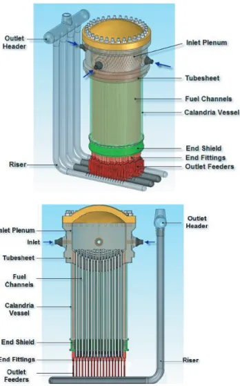
Figure 2.1 Reactor core: outside view (top) and inside view (bottom) . . . 20

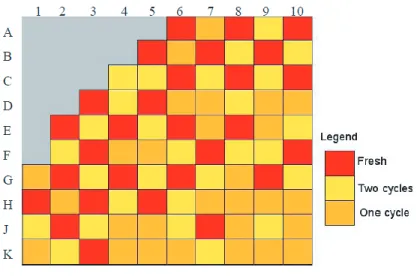
Figure 2.2 Fuel loading map . . . 21

Figure 2.3 Power calculation procedure . . . 25

Figure 2.4 Thermalhydraulics calculation procedure . . . 27

Figure 2.5 Flow chart of coupling calculations . . . 29

Figure 2.6 Comparison of density (top) and temperature (bottom) obtained from THERMO: and AECL . . . 31

Figure 2.7 Comparison of bundle power obtained from THERMO (top) and AECL (bottom) . . . 33

Figure 2.8 Comparison of coolant and cladding temperatures obtained from THERMO: (top) and AECL (bottom) . . . 34

Figure 3.1 Values of the Kef f during iterations . . . 36

Figure 3.2 Channel-power distribution at convergence . . . 37

Figure 3.3 Bundle power at the first 4 iterations . . . 38

Figure 3.4 Bundle power at convergence . . . 39

Figure 3.5 Specific-heat capacity at the first 4 iterations . . . 40

Figure 3.6 Specific-heat capacity at convergence . . . 40

Figure 3.7 Heat-transfer coefficient at the first 4 iterations . . . 41

Figure 3.8 Heat-transfer coefficient at convergence . . . 42

Figure 3.9 Coolant temperature at the first 4 iterations . . . 43

Figure 3.11 Coolant density at the first 4 iterations . . . 44

Figure 3.12 Coolant density at convergence . . . 45

Figure 3.13 Pressure at the first 4 iterations . . . 46

Figure 3.14 Pressure at convergence . . . 46

Figure 3.15 Data at convergence; heat-transfer (H-T) coefficient in 100 W·(m2_{· K)}−1 ₄₇ Figure 3.16 Bundle power at the first 4 iterations . . . 48

Figure 3.17 Bundle power at convergence . . . 49

Figure 3.18 Specific-heat capacity at the first 4 iterations . . . 50

Figure 3.19 Specific-heat capacity at convergence . . . 50

Figure 3.20 Heat transfer coefficient at the first 4 iterations . . . 51

Figure 3.21 Heat-transfer coefficient at convergence . . . 52

Figure 3.22 Coolant temperature at the first 4 iterations . . . 53

Figure 3.23 Coolant temperature at convergence . . . 53

Figure 3.24 Coolant density at the first 4 iterations . . . 54

Figure 3.25 Coolant density at convergence . . . 55

Figure 3.26 Pressure at the first 4 iterations . . . 56

Figure 3.27 Pressure at convergence . . . 56

Figure 3.28 Data at convergence; heat-transfer coefficient in 100 W·(m2· K)−1 _{. . . 57}

Figure 3.29 Bundle power at the first 4 iterations . . . 58

Figure 3.30 Bundle power at convergence . . . 59

Figure 3.31 Specific-heat capacity at the first 4 iterations . . . 60

Figure 3.32 Specific-heat capacity at convergence . . . 60

Figure 3.33 Heat-transfer coefficient at the first 4 iterations . . . 61

Figure 3.34 Heat-transfer coefficient at convergence . . . 62

Figure 3.35 Coolant temperature at the first 4 iterations . . . 63

Figure 3.36 Coolant temperature at convergence . . . 63

Figure 3.37 Coolant density at the first 4 iterations . . . 64

Figure 3.38 Coolant density at convergence . . . 65

Figure 3.39 Pressure drop at the first 4 iterations . . . 66

Figure 3.40 Pressure at convergence . . . 66

LIST OF APPENDICES

Appendix A DONJON input files . . . 71 Appendix B DRAGON input files for reactivity-coefficient calculations . . . 99 Appendix C DRAGON input files for database generation . . . 117

LIST OF ACRONYMS AND ABREVIATIONS

P Power

˙

m Mass flow rate

q′′ Heat flux

q′′′ Power density

Q1 Heat transfer rate from fuel to cladding Q2 Heat transfer rate from cladding to coolant Vf Fuel volume

Vg Cladding volume

Af Fuel surface area

Ag Cladding surface area

hc Coolant heat transfer coefficient

hgap Gap conductance between fuel and cladding

H Enthalpy

cp Specific-heat capacity of the coolant

Nrod Number of fuel rods per bundle

Rrod Radius of each fuel rod

kc Coolant thermal conductivity

G Mass flux

f Single-phase friction factor

tf Fuel temperature

tg Cladding temperature

ρc Coolant density

Kef f Effective multiplication factor

p Coolant pressure

AECL Atomic Energy of Canada Limited

νΣf Product of the macroscopic fission cross section to the average number of neutrons produced by fission

Σ Total macroscopic fission cross section

Dh Hydraulic diameter

Pwet Wetted perimeter

Dhe Heated equivalent diameter

Phe Heated perimeter

nR1 Number of fuel elements in Ring 1

N u Nusselt number

P r Prandtl number

nR2 Number of fuel elements in Ring 2

nR3 Number of fuel elements in Ring 3

Dc Diameter of central pin including cladding

DR1 Outer diameter of pins in Ring 1

DR2 Outer diameter of pins in Ring 2

DR3 Outer diameter of pins in Ring 3

Dliner Inner diameter of liner

Af low Flow area

µ Dynamic viscosity

cpf Specific heat-capacity of the fuel

cpg Specific heat-capacity of the cladding

INTRODUCTION

In order to implement new nuclear technologies as a solution to the growing demand for energy, 10 countries agreed on a framework for international cooperation in 2002, to form the Generation IV International Forum (GIF). The goal of the GIF is to design the next genera-tion of nuclear reactors that would be cost effective and would enhance safety. This forum has proposed several types of Generation IV reactors including the Supercritical Water-Cooled Reactor (SCWR). The SCWR comes in two main configurations: pressure vessel SCWR and pressure tube SCWR (PT-SCWR).

Several neutronics/thermalhydaulics coupling studies have been performed on the CANDU SCWR (a PT-SCWR) to understand its properties. Shan et al. (2009a) studied the effects of fuel enrichment and of the lattice pitch on the power distribution within a channel. The chan-nel consisted of the 43-rod CANFLEX bundle, and the coupling was done through MCNP (Briesmeister, 2000) and ATHAS (Shan et al., 2009b). To analyze the effects of fuel enrich-ment, two cases were considered: a reference case and an improved case. In the reference case, all fuel rods were assumed to be made of UO2 enriched to 4% in U235. The results showed

that, for each fuel bundle, the power was not evenly distributed across all sub-channels, with the power peak located next to the outer sub-channels. Also, the heat-transfer coefficient was relatively low around this region. Therefore, the cladding temperatures in some outer sub-channels exceeded the allowed cladding temperature. To solve this problem, Shan et al. (2009a) proposed an improved case in which the fuel rods in rings 1, 2, 3, and 4 would be enriched to 6%, 6%, 5%, and 2.5%, respectively. As a result, the radial power in each bundle was more evenly distributed, and the cladding temperatures were within the allowable limit. They concluded the study by showing that lower values of the lattice pitch resulted in a more uniform radial power distribution in a channel.

The 43-rod CANFLEX bundle was intended to be used in a horizontal CANDU SCWR, similar to a CANDU 6 reactor, with online refueling. However, it was determined that online refueling was not an easy option with supercritical water. Consequently, high-burnup bundle designs were considered so as not to use online refueling and to allow longer refueling cycles. Nevertheless, the use of high-burnup fuel imposed severe contraints on the linear element rating (LER) due to the accumulation of fission gases between the fuel and the cladding, as the fuel is irradiated (MacDonald et al., 2011). MacDonald et al. (2011) performed a neutron-ics/thermalhydaulics coupling study to calculate the linear element rating for three bundle designs. The first one was the 54-element-bundle design that consisted of one non-fuel rod in the center surrounded by 54 fuel rods arranged in 3 rings of 12, 18, and 24 rods, respectively.

Also, the design used fuel rods of the same diameter. The second design had 79 rods per bundle, out of which only the central pin did not contain fuel. The central pin in this case was surrounded by 3 rings of 15, 21, and 42 elements, respectively. The fuel rods in the outer ring had a smaller diameter in order to reduce their LER. As Shan et al. (2009a) had shown, the fuel rod in the outer ring would generate the maximum power in the bundle. Therefore, it would be important to impose a restriction on their diameter to insure their LER had an acceptable value. The third design had 51 rods with one non-fuel rod at the center and 50 fuel rods arranged in 3 rings of 12, 18, and 20 rods, respectively. Once again, the focus in this design was on the outer ring. This design would reduce the LER in this ring by using fuel rods with an annular shape (having a hole at the center in which the coolant flows) In all three designs, a homogeneous fuel composition of Thorium Oxyde with 12% Plutonium Oxyde was considered. MacDonald et al. (2011) concluded that the 79-rod design gave the lowest LER for a burnup of up to 40MWD/Kg.

It this study, the vertically-oriented CANDU SCWR is analyzed. It contains 336 chan-nels with a length of 5 m. The target coolant inlet and outlet temperatures are 350 C and 625 C, respectively. The coolant flows downwards at a pressure above the critical pressure, and the reactor power is 2540 MWth.

The aim of this study is to use the neutronics-thermalhydraulics coupling method to de-termine the core-power distribtution and the thermalhydraulics parameters of a CANDU SCWR. To this end, Chapter 1 gives a description of the SCWR-cell model and of the reactor-database generation process. Chapter 2 presents the reactor-core model, the steady-state thermalhydraulics and heat-transfer models, and the coupling algorithm. In Chapter 3, the results obtained for selected channels are conveyed. Finally, a discussion of the signif-icance of the results concludes the study.

CHAPTER 1

CANDU SCWR CELL AND REACTOR DATABASE

The implementation of a neutronics/thermalhydraulics coupling scheme relies on the use of a reactor-cell model to generate the cross-section database for full-core calculations. The cell model also gives information about the dependence of the effective multiplicative factor on local and global parameters. This chapter gives a description of the cell model, analyzes the effects of local parameters (fuel temperature, coolant temperature, and coolant density) on the effective multiplication factor, and gives details about the reactor-database generation process.

1.1 Cell-model description

The reactor-cell model used is presented in Figure 1.1, and its parameters are given in Table 1.1 (Pencer, 2008). It has 54 fuel rods organized in 3 rings having 12, 18, and 24 elements, respectively. The center pin contains light water surrounded by cladding. Table 1.2 gives details about its composition (Pencer, 2008); in this table, the isotopic content of the PuO2 is 2.5%, 54.2%, 23.8%, 12.6%, and 6.8% in Pu238, Pu239, Pu240, Pu241, and Pu242, respec-tively.

The CANDU SCWR cell differs from the CANDU 6 cell in many aspects. The CANDU SCWR cell has more fuel rods per bundle, and uses an insulator and a liner to seperate the pressure tube from the coolant. The insulator is used to prevent damage to the pressure tube resulting from the high-temperature coolant, and the liner protects the insulator from being damaged during channel refueling. The CANDU SCWR cell also has a central pin whose goal is to reduce the coolant-void reactivity. Due to the presence of the high-temperature coolant, the cladding is made of stainless steel, instead of Zirconium.

1.2 Cell neutronics properties

The multigroup transport equation is given by (H´ebert, 2008)

Table 1.1 CANDU SCWR channel parameters

Parameter Value Parameter Value

Pitch circle radius, ring 1 2.8755 cm Lattice pitch 25 cm

Pitch circle radius, ring 2 4.3305 cm Pressure tube inner radius 8.23 cm Pitch circle radius, ring 3 5.8000 cm Pressure tube thickness 1.4 cm

Radius of central pin 1.8 cm Liner tube inner radius 6.8 cm

Outer radius of central pin cladding 2.0 cm Liner tube thickness 0.1 cm Radius of pins in ring 1, 2 and 3 0.620 cm Insulator inner radius 6.9 cm Outer radius of ring 1, 2 and 3 pin cladding 0.660 cm Insulator thickness 1.33 cm

Table 1.2 Cell composition

Material Composition

Fuel rods 88 wt% ThO2, 12 wt% PuO2

Cladding (center pin and rings 1, 2, and 3) 310 Stainless Steel

Liner 30% 310 Stainless Steel, 70% Coolant

Insulator 30% ZrO2, 70% Coolant

Pressure tube Zr-2.5Nb

Coolant H2O

Moderator D2O

Moderator Fuel Cladding Pressure tube

Liner Insulator Coolant

Figure 1.1 CANDU SCWR cell with 54 fuel elements per bundle

where 1 ≤ g ≤ G, and Qg(r, Ω) = G ∑ h=1 L ∑ l=0 2l + 1 4π Σs,l,g←h(r) l ∑ m=−l Rm_l (Ω)ϕm_l,h(r) + 1 4πKef f J ∑ j=1 χj,g G ∑ h=1 νΣf,j,h(r)ϕh(r) (1.2) χj,g = ∫ ug ug−1 χj(u)du (1.3)

In order to determine the properties of the CANDU SCWR cell and to generate the cross-section database required in subsequent full-core calculations, the version 3.06K of the DRAGON code is used (Marleau et al., 2008). The multigroup transport equation is solved (with the assumption of isotropic scattering) by the method of collision probability, using the ENDF/B-VII nuclear library. A coarse geometry is used for self-shielding calculations, and a fine-mesh geometry is chosen for flux calculations (Figure 1.2). The flux obtained is used to homogenize cross sections over the entire cell and to condense them into 2 energy groups with a boundary of 0.625 eV (Harrisson and Marleau, 2011).

1.2.1 Effect of burnup on reactivity

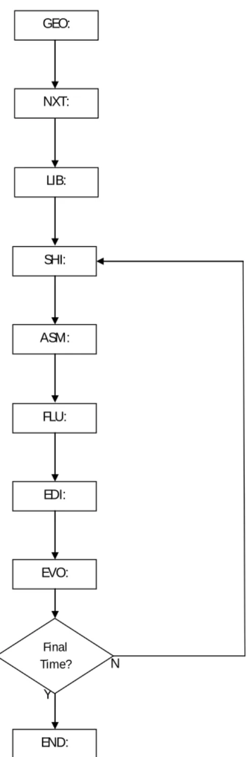
A lattice calculation (Figure 1.3) is done to analyse the impact of burnup on reactivity. The GEO: module defines two geometries (Figure 1.2). The NXT: module creates integration lines in both geometries. The LIB: module creates a microlib data structure that contains both microscopic and macroscopic cross sections for all reactions types and for all the iso-topes considered. The microlib is generated based on the parameters given in Table 1.3. The SHI: module then performs resonance self-shielding calculations on the microlib, by using the coarse geometry. The collision probability matrices are calculated by the ASM: module, based on the self-shielded cross sections and the fine geometry. Once the collision probability matrices are known, the FLU: module determines the flux, along with the Kef f, and the EDI: module uses the flux to homogenize cross sections, over the entire cell, and to con-dense them into two energy groups. By using the specified bundle power and time step, the EVO: module solves the isotope evolution equations to determine their new concentrations; the new concentrations are added to the microlib. If the final simulation time is reached, the END: module terminates the DRAGON program; otherwise, the SHI: module performs self-shielding calculations on the new microlib data structure, and the computations continue according to Figure 1.3.

Once the Kef f is known, the reactivity ρmk is given by

ρmk =

(Kef f − 1) · 1000

Kef f

(1.4)

In Figure 1.4, the reactivity starts at 149.1 mk with fresh fuel and decreases with time due to Table 1.3 Reference database parameters

Fuel temperature (K) 1273.15 Moderator purity (%) 99.833

Coolant temperature (K) 923.15 Boron concentration (cm· b)−1 1.0E-10 Moderator temperature (K) 342.16 Xenon concentration (cm· b)−1 1.0E-24 Coolant density (g· cm−3) 0.35 Samarium concentration(cm· b)−1 1.0E-24 Moderator density (g· cm−3) 1.08509 Neptunium concentration (cm· b)−1 1.0E-24

Coolant purity (%) 0.0156 Bundle power (MW) 0.75595

burnup. The reactivity is not less than 0 for burnup values up to approximately 25 MWD/Kg.

N Y GEO: NXT: LIB: SHI: ASM: FLU: EDI: EVO: END: Final Time?

0 5 10 15 20 25 30 35 40 45 −100 −50 0 50 100 150 Burnup (MWD/Kg) Reactivity (mk)

Figure 1.4 Reactivity as a function of burnup

coolant density on reactivity, are presented. In each case, the calculation scheme of Figure 1.3 is used, and only the parameter being analyzed (fuel temperature, coolant temperature, or coolant density) is varied, while all the other local and global parameters are kept at their reference values (Table 1.3). However, in all cases, the burnup is allowed to vary.

1.2.2 Effect of the fuel temperature on reactivity

The reactivity decreases with an increase in the fuel temperature due to the doppler effect (Figures 1.5). However, the fuel-temperature coefficient increases with burnup. The average fuel-temperature coefficients are -2.0602 mk/K, -1.8952 mk/K, and -1.6589 mk/K for

0 MWD/Kg, 15 MWD/Kg, and 25 MWD/Kg, respectively. These values are calculated from Figure 1.5 by the expression ∆ρmk

∆tf . The fuel-temperature coefficient decreases with the

burnup probably because of the creation of U233 from Th232, and the fission cross section of U233 may counter the doppler effect.

1.2.3 Effect of the coolant temperature on reactivity

The coolant-temperature coefficient decreases with an increase in the coolant temperature. Also the sign of the coolant-temperature coefficient changes, but the temperature at which this transition occurs depends on the burnup (Figures 1.6). The change in the sign of the

600 800 1000 1200 1400 1600 1800 135 140 145 150 155 160 165 Temperature (K) Reactivity (mk) Burnup = 0 600 800 1000 1200 1400 1600 1800 45 50 55 60 65 Temperature (K) Reactivity (mk) Burnup = 15 MWJ/Kg 600 800 1000 1200 1400 1600 1800 −2 0 2 4 6 8 10 12 14 16 Temperature (K) Reactivity (mk) Burnup = 25 MWJ/Kg

coolant-temperature coefficient could be the result of peaks in the fission cross sections of Pu239 and U233 at 0.3 eV and 200 keV, respectively. Increasing the coolant temperature increases the energy of neutrons, and some of them have energy transitions past these reso-nance energies. For fresh fuel, the resoreso-nance of Pu239 is the main contributor. As the fuel burnup increases, more U233 is created and less Pu239 is present; therefore, U233 becomes more significant, and the transition temperature for the coolant-temperature coefficient in-creases. For fresh fuel, the transition happens at T = 412.5 K, whereas for 15 MWD/Kg and 25 MWD/Kg the transition temperatures are T = 637.5K and T = 862.5K, respectively.

300 400 500 600 700 800 900 1000 1100 1200 148 148.5 149 149.5 Temperature (K) Reactivity (mk) Burnup = 0 MWD/Kg 300 400 500 600 700 800 900 1000 1100 1200 52.8 53 53.2 53.4 53.6 53.8 54 54.2 54.4 54.6 Temperature (K) Reactivity (mk) Burnup = 15 MWD/Kg 300 400 500 600 700 800 900 1000 1100 1200 4.4 4.6 4.8 5 5.2 5.4 5.6 5.8 6 Temperature (K) Reactivity (mk) Burnup = 25 MWD/Kg

1.2.4 Effect of the coolant density on reactivity

The coolant-density coefficient increases with an increase in the coolant density. Also the sign of the coolant-density coefficient changes, but the density at which this transition occurs does not depend on the burnup (Figures 1.7): the transition density in all three cases is determined to be ρc = 0.0875 g/cm3. For densities ρc ≥ ρref, the calculated values of the coolant density coefficients are 39.4 mk/g·cm3_{, 47.4 mk/g}·cm3_{, and 45.1 mk/g}·cm3 _{for 0}

MWD/Kg, 15 MWD/Kg, and 25 MWD/Kg, respectively. In this case, the coolant-density coefficients are the values of ∆ρmk

∆tc , calculated from Figure 1.7. Moreover, the coolant void

fraction is negative since

ρmk(ρc = 10−3 g/cm3) - ρmk(ρc) < 0 ∀ρc such that ρc ≥ ρref, where ρref is the reference coolant density given in Table 1.3.

0 0.1 0.2 0.3 0.4 0.5 0.6 0.7 144 146 148 150 152 154 156 158 160 162 164 Coolant density (g/cc) Reactivity (mk) Burnup = 0 MWD/Kg 0 0.1 0.2 0.3 0.4 0.5 0.6 0.7 45 50 55 60 65 70 75 Coolant density (g/cc) Reactivity (mk) Burnup = 15 MWJ/Kg 0 0.1 0.2 0.3 0.4 0.5 0.6 0.7 −5 0 5 10 15 20 25 Coolant density (g/cc) Reactivity (mk) Burnup = 25 MWD/Kg

1.3 Reactor-database generation

The generation of a reactor database can be done in three stages.

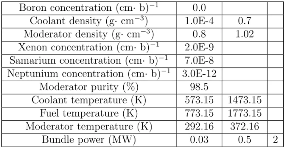
The first stage consists of creating a fixed-parameter database with each parameter fixed at its reference value (Table 1.3). More fixed-parameter databases are created during the second stage with the use of perturbation values (Table 1.4). It is worth mentioning that in the first two stages, the computations are performed according to Figure 1.8; this is similar to Figure 1.3, with the exception that the CPO: module is used to generate the databases. Finally, in the last stage, the CFC: module combines all the databases, resulting from the first two stages, into a single variable-parameter database for full-core calculations (Figure 1.9).

Table 1.4 Perturbation database parameters

Boron concentration (cm· b)−1 0.0

Coolant density (g· cm−3) 1.0E-4 0.7 Moderator density (g· cm−3) 0.8 1.02 Xenon concentration (cm· b)−1 2.0E-9

Samarium concentration (cm· b)−1 7.0E-8 Neptunium concentration (cm· b)−1 3.0E-12

Moderator purity (%) 98.5

Coolant temperature (K) 573.15 1473.15

Fuel temperature (K) 773.15 1773.15

Moderator temperature (K) 292.16 372.16

Bundle power (MW) 0.03 0.5 2

The database parameters are not all determined in the same way:

• The Boron concentrations are selected to agree with the fact that no Boron will be used

in core calculations.

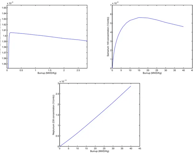
• The Xenon, Samarium, and Neptunium concentrations are determined through a lattice

calculation that determines their maximum values during the reactor operating cycle, as indicated in Figure 1.10.

• The maximum and minimum values of the bundle power, fuel temperature, coolant

temperature, and coolant density are selected so that their values in the core, obtained with the neutronics/thermalhydraulic coupling, are within these boundaries: these val-ues are selected so that they represent upper/lower bounds for the bundle power, fuel temperature, coolant temperature, and coolant density values obtained with the neu-tronics/thermalhydraulics coupling to be discussed in the next chapter.

N Y GEO : NXT : LIB: SHI : ASM : FLU : EDI: EVO : CPO : Final Time? END :

Figure 1.9 Calculation scheme for the generation of a variable-parameter database 0 0.5 1 1.5 2 2.5 1.55 1.56 1.57 1.58 1.59 1.6 1.61 1.62 1.63 1.64 1.65 x 10−9 Burnup (MWD/Kg) Xenon 135 concentration (1/(cmb)) 0 5 10 15 20 25 30 35 40 45 0 1 2 3 4 5 6 7x 10 −8 Burnup (MWD/Kg) Samarium 149 concentration (1/(cmb)) 0 5 10 15 20 25 30 35 40 45 0 0.5 1 1.5 2 2.5 3x 10 −12 Burnup (MWD/Kg) Neptunium 239 concentration (1/(cmb))

1.4 Reactor-database validation

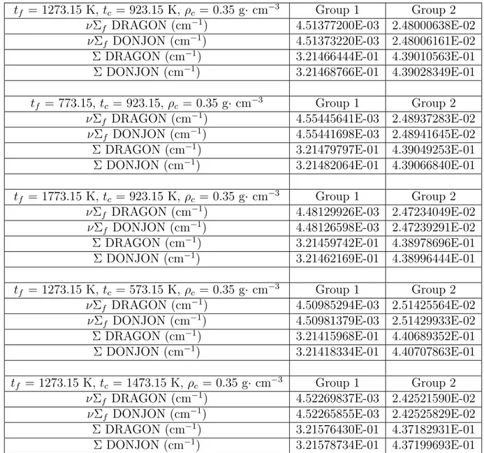
In order to validate the reactor database, a comparison between the macroscopic cross sec-tions obtained with DRAGON and DONJON (Varin et al., 2005) are compared. Different simulation conditions are selected, corresponding to reference conditions or perturbation con-ditions. The DRAGON macroscopic cross section data is generated by the CPO: module, while the DONJON macroscopic cross section data is generated by the AFM: module. The results show a very good agreement between the cross sections resulting from DRAGON and DONJON (Tables 1.5 and 1.6). To determine the difference in channel power resulting from the use of the CPO: and the AFM: cross sections, the core power is calculated under the following conditions:

• Simulation condition 1: tf = 1273.15 K, tc = 923.15 K, ρc = 0.0001 g· cm−3

Table 1.5 Database validation (Part 1)

tf = 1273.15 K, tc = 923.15 K, ρc = 0.35 g· cm−3 Group 1 Group 2

νΣf DRAGON (cm−1) 4.51377200E-03 2.48000638E-02

νΣf DONJON (cm−1) 4.51373220E-03 2.48006161E-02

Σ DRAGON (cm−1) 3.21466444E-01 4.39010563E-01

Σ DONJON (cm−1) 3.21468766E-01 4.39028349E-01

tf = 773.15, tc = 923.15, ρc = 0.35 g· cm−3 Group 1 Group 2

νΣf DRAGON (cm−1) 4.55445641E-03 2.48937283E-02

νΣf DONJON (cm−1) 4.55441698E-03 2.48941645E-02

Σ DRAGON (cm−1) 3.21479797E-01 4.39049253E-01

Σ DONJON (cm−1) 3.21482064E-01 4.39066840E-01

tf = 1773.15 K, tc = 923.15 K, ρc = 0.35 g· cm−3 Group 1 Group 2

νΣf DRAGON (cm−1) 4.48129926E-03 2.47234049E-02

νΣf DONJON (cm−1) 4.48126598E-03 2.47239291E-02

Σ DRAGON (cm−1) 3.21459742E-01 4.38978696E-01

Σ DONJON (cm−1) 3.21462169E-01 4.38996444E-01

tf = 1273.15 K, tc = 573.15 K, ρc = 0.35 g· cm−3 Group 1 Group 2

νΣf DRAGON (cm−1) 4.50985294E-03 2.51425564E-02

νΣf DONJON (cm−1) 4.50981379E-03 2.51429933E-02

Σ DRAGON (cm−1) 3.21415968E-01 4.40689352E-01

Σ DONJON (cm−1) 3.21418334E-01 4.40707863E-01

tf = 1273.15 K, tc = 1473.15 K, ρc = 0.35 g· cm−3 Group 1 Group 2

νΣf DRAGON (cm−1) 4.52269837E-03 2.42521590E-02

νΣf DONJON (cm−1) 4.52265855E-03 2.42525829E-02

Σ DRAGON (cm−1) 3.21576430E-01 4.37182931E-01

Table 1.6 Database validation (Part 2)

tf = 1273.15 K, tc = 923.15 K, ρc = 0.0001 g· cm−3 Group 1 Group 2

νΣf DRAGON (cm−1) 3.80233530E-03 2.57132040E-02

νΣf DONJON (cm−1) 3.66699745E-03 2.59954415E-02

Σ DRAGON (cm−1) 2.82237007E-01 4.14263243E-01

Σ DONJON (cm−1) 2.75949165E-01 4.04561347E-01

tf = 1273.15 K, tc = 923.15 K, ρc = 0.7 g· cm−3 Group 1 Group 2

νΣf DRAGON (cm−1) 4.88468069E-03 2.55906676E-02

νΣf DONJON (cm−1) 4.91055898E-03 2.58561428E-02

Σ DRAGON (cm−1) 3.60683613E-01 4.72757666E-01

Σ DONJON (cm−1) 3.66969935E-01 4.85383192E-01

tf = 528.501 K, tc = 416.3884 K, ρc = 0.264086 g· cm−3 Group 1 Group 2

νΣf DRAGON (cm−1) 4.44213714E-03 2.53161277E-02

νΣf DONJON (cm−1) 4.41257098E-03 2.52200373E-02

Σ DRAGON (cm−1) 3.11764035E-01 4.34029735E-01

Σ DONJON (cm−1) 3.10630768E-01 4.36999036E-01

tf = 1028.5 K, tc = 805.0995 K, ρc = 0.1938247 g· cm−3 Group 1 Group 2

νΣf DRAGON (cm−1) 4.26642017E-03 2.49514516E-02

νΣf DONJON (cm−1) 4.20798628E-03 2.51534902E-02

Σ DRAGON (cm−1) 3.03934086E-01 4.27176837E-01

Σ DONJON (cm−1) 3.01729445E-01 4.32215285E-01

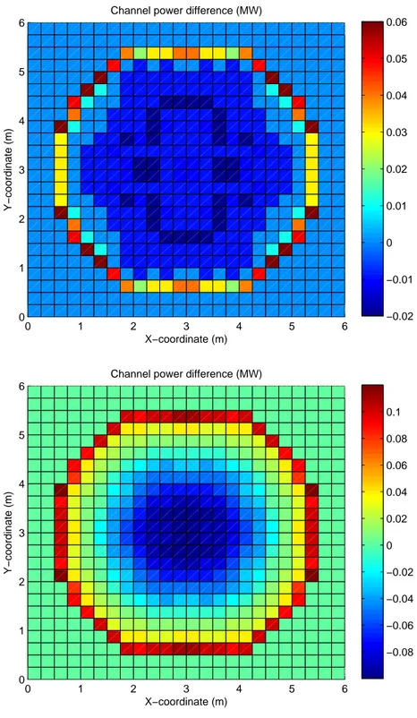
In Figure 1.11, the maximum error occurs at outer channels, and has a value of 3.5% of the channel power where it occurs; the power of this channel is 3.02 MW.

0 1 2 3 4 5 6 0 1 2 3 4 5 6 X−coordinate (m) Channel power difference (MW)

Y−coordinate (m) −0.02 −0.01 0 0.01 0.02 0.03 0.04 0.05 0.06 0 1 2 3 4 5 6 0 1 2 3 4 5 6 X−coordinate (m) Channel power difference (MW)

Y−coordinate (m) −0.08 −0.06 −0.04 −0.02 0 0.02 0.04 0.06 0.08 0.1

Figure 1.11 Difference in channel power (CPO results - AFM results) for Simulation condition 1 (top) and Simulation condition 2 (bottom)

CHAPTER 2

STEADY-STATE ANALYSIS

After generating and validating the cross-section database, the next step is to implement a reactor-core model, a thermalhydraulics model, a heat-transfer model, and a neutron-ics/thermalhydaulics coupling methodology.

2.1 Reactor-core model

Figure 2.2 Fuel loading map

The reactor is made of 336 channels of 5 m in length. It has a vertical orientation, and the coolant flows downward. As Figure 2.1 shows, the coolant enters the inlet plenum through inlet pipes. It spreads across all channels in such a way as to maintain an even channel input mass-flow rate and temperature. It then flows through the channels all the way to the outlet header (MacDonald et al., 2011).

In contrast to the CANDU 6 reactor, this reactor design does not support online refueling, and one possible reason for this choice is the need for a new refueling machine design to deal with supercritical water. As a result, the designers of this reactor plan on using a three-batch scheme in which one third of the core contains fresh fuel, one third contains fuel having spent a loading cycle in the core, and the remaining third has fuel having spent two loading cycles. The cycle length depends on the fuel composition, and the designers chose the fuel arrangement of Figure 2.2 so as to minimize the power peaking factor (MacDonald et al., 2011).

Although the designers intent to use a three-batch scheme, the present study is done with the assumption that the core is filled with fresh fuel; furthermore, neither reactivity control mechanisms nor burnable absorbers are taken into account.

2.2 Thermalhydraulics and heat-transfer models

In order to perform a thermalhydaulics and heat-transfer analysis, the THERMO: module (Adouki, 2011) has been included in the DONJON code. Let z be an axial location mea-sured from the channel inlet; the module determines the fuel temperature tf(z), the cladding temperature tg(z), the coolant pressure p(z), the coolant density ρc(z), and the coolant

tem-perature tc(z) at the axial location z from p(0), ˙m, q

′′

(z), ρc(0), and tc(0). Solving this problem requires models for thermalhydraulics and heat-transfer. The following models are known to give satisfactory results:

• 1-D model for thermalhydaulics (Tapucu, 2009).

• Doubly-lumped parameter model for heat-transfer (Lewis, 1977).

During constant-power conditions, the core-power distributions changes; therefore, thermal-hydaulics parameters change with time. However, their rates of change are so small that they can be ignored, as it is commonly done. As a result, steady-state models for thermalhydaulics and heat transfer are used in this chapter.

2.2.1 Thermalhydaulics model

The 1-D thermalhydaulics model is based on the following conservation laws:

• Mass: ˙ m(z) = constant (2.1) • Momentum: dP (z) dz =− f G2 2ρc(z)Dh − G2d ( 1 ρc(z) ) dz + ρc(z)g (2.2) • Energy: dH(z) dz = 2πq′′(z)RrodNrod ˙ m (2.3)

Not having an adequate correlation for the friction factor f , the following assumption is made:

− f G2

2ρc(z)Dh + ρc(z)g = 0 (2.4)

so that the momentum conservation becomes:

dP (z) dz =−G 2d ( 1 ρc(z) ) dz (2.5)

Applying the conservation laws between z and z + ∆z, for ∆z small, gives for the monentum equation P (z + ∆z) = P (z)− G2 ( 1 ρ(z + ∆z)− 1 ρ(z) ) (2.6)

while the energy equation becomes H(z + ∆z)− H(z) = 2πq ′′ (z)∆zRrodNrod ˙ m (2.7) The relation H(z + ∆z)− H(z) = cp(z) (tc(z + ∆z)− tc(z)) (2.8) gives tc(z + ∆z) = 2πq′′(z)∆zRrodNrod ˙ mcp(z) + tc(z) (2.9)

The heat-transfer coefficient is

hc(z) =

kc(z)N u(z)

Dhe

(2.10) From (MacDonald et al., 2011), we obtain that:

N u(z) = 0.023Re0.8(z)P r0.4(z) (2.11) Dhe = 4Af low Phe (2.12) Phe = π (Dc+ nR1DR1+ nR2DR2+ nR3DR3) (2.13) Af low= π 4 ( D_liner2 − D_c2− nR1DR12 − nR2D2R2− nR3DR32 ) (2.14) Dh = 4Af low Pwet (2.15) Pwet= π (Dliner+ Dc+ nR1DR1+ nR2DR2+ nR3DR3) (2.16) P r(z) = cp(z)µ(z) kc(z) (2.17) 2.2.2 Heat-transfer model

The heat-transfer model is based on the doubly-lumped parameter model, and it has the following attributes:

• It neglects the axial heat transfer along the fuel and the cladding.

• Instead of using tf(z, r) and tg(z, r), it uses their channel-averaged values in the radial direction, between z and z +∆z, denoted by tf(z) and tg(z), respectively.

By using the energy balance in the fuel and in the cladding, between z and z + ∆z, we obtain for each fuel rod:

q′′′(z)Vf − Q1(z) = 0 Q1(z)− Q2(z) = 0 Q2(z) = hc(z)Ag[tg(z)− tc(z)] Q1(z) = Afhgap[tf(z)− tg(z)] Therefore, tg(z) = q ′′′ (z)Vf hc(z)Ag + tc(z) (2.18) tf(z) = q′′′(z)Vf hg(z)Af + tg(z) (2.19)

2.3 Reactor-power calculation procedure

The multigroup steady state diffusion equation is given by (H´ebert, 2008)

− ∇ · Dg(r)∇ϕg(r) + Σg(r) = Qg(r) (2.20)

The source term is

Qg(r) = G ∑ h=1 Σg←h(r)ϕg(r) + χg(r) Kef f G ∑ h=1 νΣf h(r)ϕh(r) (2.21)

The reactor core model is implemented with the 3-D diffusion code DONJON version 3.02B (Varin et al., 2005), and calculations are performed with two energy groups. Each channel is partitioned into 10 cells of length, width, and height 25 cm, 25 cm, and 50 cm, respectively. The flux in each cell is determined by the Mesh-Centered-Finite-Difference Approximation. At the onset of a power calculation (Figure 2.3), the GEOD: creates the core geometry which consists of 10 planes of 576 cells each, 336 cells of which are fuel ones. The USPLIT: module performs mesh splitting on the geometry and determines new mixtures indices so that every mixture index corresponds to only one sub-region. After the mesh splitting is completed, the TRIVAT: module performs a TRIVAC-type tracking on the geometry, and the geometry is then used by the INIRES: module to create a fuel map. The fuel map contains information on each fuel cell, such as fuel burnup, fuel power, fuel temperature, coolant temperature, and

coolant density. The REFRES: module establishes a correspondance between the calculation geometry, the material indices, and the fuel map; this singles out indices that refer to mixtures in fuel cells from indices that do not. By using the information about each cell, the AFM: module creates two macroscopic cross sections data structures: one for fuel cells and the other one for reflector cells. These data structures are combined into a single one by the UNIMAC: module, and this allows the TRIVAA: module to create systems matrices necessary for flux calculations. The FLUD: module determines the flux distribution in the core, which is then averaged over each cell by the FLXAXC: module. Finally, the POWER: module uses the average flux and the total core power, to determine the power in each cell.

2.4 Thermalhydraulics calculation procedure

The goal of the new THERMO: module is to determine, for each channel, the fuel temperature

tf(z), the cladding temperature tg(z), the coolant pressure p(z), the coolant density ρc(z), and the coolant temperature tc(z) at the axial location z from p(0), ˙m, q

′′

(z), ρc(0), and tc(0). The module uses the finite-volume method, the conservation laws, and the NIST Standard Reference Database 23 (NIST, 2011) to determine the unknown parameters. Calculations are based on the value of hgap = 10 kW/m2/oC (Rozon, 1998) and the channel design parameters depicted in Table 2.1 (MacDonald et al., 2011). The algorithm of the module is given in Figure 2.4. It is based on the assumption that an equation of state, giving all the thermodynamic properties of water, is available. Thus, after selecting a channel, the module determines

hc(z), tg(z), and tf(z) from tc(z) and p(z) by using equations 2.10 through 2.19. tc(z + ∆z) is calculated from equation 2.9 by using p(z), tc(z), and the bundle powers for the channel being analyzed, and equations 2.10 through 2.20 allow the calculation of hc(z + ∆z), tg(z + ∆z), and tf(z + ∆z) from tc(z + ∆z) and p(z). Finally, Equation 2.6 gives p(z + ∆z) from p(z) and tc(z + ∆z).

Table 2.1 Channel design parameters

Parameter Value

Inlet pressure (MPa) 26

Inlet temperature (o_{C) 350} Channel massflow rate (Kg/s) 3.89

2.5 Description of the neutronics/thermalhydraulics coupling procedure

The THERMO: module exchanges data with the rest of the DONJON code, through the fuel map file that contains the data for each cell (Figure 2.5 top). In Figure 2.5 (bottom), the method starts with a core-power calculation performed from the default thermalhydaulics parameters given in Table 2.2. The resulting bundle powers are saved into the fuel map. Bundle powers are then read from the fuel map, and the THERMO: module determines the coolant temperature, the coolant density, and the fuel temperature of each cell, and this data is saved into the fuel map. The fuel temperature, coolant temperature, and coolant density of each bundle are then read, and bundle powers are computed through a full-core calculation, based on the temperature and density data of each cell; the AFM: module uses this data to determine the cross sections of each cell. The resulting bundle powers are again saved. This process is repeated until the convergence of the effective multiplication factor is reached. Note: In Figure 2.5, the initialization kef f(i−1) = 0 is done so as to ensure that at least the

second iteration is performed.

Table 2.2 Default local and global parameters for the THERMO: module Material Density (Kg/m3) Temperature (K)

Fuel N.A. 1273.15

Coolant (light water) 350 923.15

A B

D Fuel map C THERMO :

Power calculation Y N

Start

to default values

Perform power calculation

Perform power calculation Read bundle powers

Run THERMO : module Initialization

k-eff(i-1)= 0

| k-eff(i)ʹ k-eff(i-1)| < ɸ

Read THERMO : output

i = i + 1 i = 1

Stop

2.6 Validation tests for the THERMO: module

In order to validate the THERMO: module, three tests are performed in which the results of the THERMO: module are compared to those of AECL.

2.6.1 Test 1

In this test, the coolant temperature and density, for the average-power channel, are used as validation parameters. First, the core power is calculated with the fuel arrangement of Figure 2.2 and homogeneous thermalhydaulics parameters. Then, the resulting coolant temperature and density are determined without a neutronics/thermalhydaulics coupling; therefore, in this channel, the power is symetrical with respect to the normal plane to the channel axis, at 2.5 m from the channel inlet. Also, the mass flow rate used is selected so as to have a coolant output temperature of 625 o_{C while a constant channel pressure of 25.1} MPa is assumed. The coolant temperature and density predicted by THERMO: agree with those calculated by AECL, within 3%. Even though both data sets agree well (Figure 2.6), the graphs obtained with the THERMO: module show some discontinuities in the slope, whereas those obtained by AECL are smooth. The discontinuities occur only between two adjacent bundles. They result from the fact that the average power of each bundle was used in thermalhydraulics calculations. From Equation 2.9, the slope of the coolant-temperature curve is given by 2πq′′(z)RrodNrod

˙

mcp(z) , and q ′′

(z) may have discontinuities at the interface of two bundles and accordingly affect the slope at these locations.

2.6.2 Test 2

This test uses the bundle powers of the maximum-power channel as the validation pa-rameter. In the case of THERMO:, the core power is determined through a neutron-ics/thermalhydraulics coupling procedure under the assumption that the core is filled with fresh fuel only. Thermalhydaulics calculations are done with a channel mass-flow rate of 3.89 Kg/s. In the case of AECL, the same neutronics/thermalhydaulics coupling method is per-formed with a channel mass-flow rate of 3.89 Kg/s and the fuel loading pattern of Figure 2.2; Figure 2.7 gives the results. The AECL graph shows results both at the beginning of cycle (blue curve) and at the end of cycle (red curve). The result comparison at the beginning of cycle indicates a power peak at the third bundle (from the channel input) in the case of THERMO: and at the fourth bundle in the case of AECL. Also, the power peak predicted by THERMO: is higher than that predicted by EACL since only fresh fuel is used in the THERMO: core model, while a combination of fresh and spent fuel is used in the AECL core model (Figure 2.2). Moreover, the use of spent fuel shifts the power peak to the right, as it

Figure 2.6 Comparison of density (top) and temperature (bottom) obtained from THERMO: and AECL

is the case for the AECL results. Therefore, the power obtained with THERMO: agrees with that obtained by EACL.

2.6.3 Test 3

This final test uses the coolant and the cladding temperatures, of the average-power channel, as validation parameters. The assumptions are similar to those of Test 2, with the exception that a constant channel pressure of 25 MPa is taken into account. In Figure 2.8, the coolant temperature predicted by THERMO: is similar to that predicted by AECL, with the exception that the peak in the temperature given by THERMO: is lightly shifted to the left of the one predicited by AECL. For the cladding temperature, both data sets show peaks next to the channel inlet; the peak predicted by THERMO: is higher than that predicted by AECL. Another observation from Figure 2.8 is that the cladding temperatures determined by THERMO:, for the last 5 bundles in the channel, are lower than their corresponding values given by AECL; this is because THERMO: predicts a bundle-power profile that is shifted to the left of the one predicted by AECL.

0 0.5 1 1.5 2 2.5 3 3.5 4 4.5 5 0 0.2 0.4 0.6 0.8 1 1.2 1.4 1.6 1.8 Axial position (m) Bundle power (MW)

0 0.5 1 1.5 2 2.5 3 3.5 4 4.5 5 0 100 200 300 400 500 600 700 800 900 Axial position (m) Temperature (K) Coolant Cladding

Cladding temperature Coolant temperature

Figure 2.8 Comparison of coolant and cladding temperatures obtained from THERMO: (top) and AECL (bottom)

CHAPTER 3

RESULTS FOR STEADY-STATE ANALYSIS

The neutronics/thermalhydraulics method, introduced in the previous chapter, is used to determine the core power and the thermalhydraulics parameters of its channels. These results are presented in this chapter.

3.1 Effective multiplication factor

Table 3.1 Effective multiplication factor

Kef f Iteration number 1.149594E+00 1 1.164142E+00 2 1.155806E+00 3 1.159475E+00 4 1.157450E+00 5 1.158354E+00 6 1.157941E+00 7 1.158120E+00 8 1.158044E+00 9 1.158075E+00 10 1.158063E+00 11 1.158068E+00 12

0 2 4 6 8 10 12 1.148 1.15 1.152 1.154 1.156 1.158 1.16 1.162 1.164 1.166 1.168 Iteration number

Effective multiplication factor

Figure 3.1 Values of the Kef f during iterations

In Table 3.1 and Figure 3.1, the value of the effective multiplication factor oscillates around the convergence value. If one iteration under-estimates the Kef f, the next one will over-estimate it, and vice-versa. This process is repeated until convergence, as the difference between successive values of the Kef f decreases. The value ϵ = 10−5is used in the convergence condition for the Kef f in Figure 2.5.

3.2 Channel-power distribution

Figure 3.2 shows that the channel power is not evenly distributed; most channels have a power larger than the average channel power (7.556 MW). The high power density at the center of the core results from the use of fresh fuel without any reactivity control mechanisms. The results are as follows:

• Maximum channel power: 10.55 MW • Minimum channel power: 4.05 MW • Power peaking factor: 1.4

0 1 2 3 4 5 6 0 1 2 3 4 5 6 X−Coordinate (m) Channel power (MW) Y−Co ord ina te ( m ) 0 1 2 3 4 5 6 7 8 9 10 Channel 5 Channel 1 Channel 10

3.3 Results for channel 1 3.3.1 Bundle power 0 0.5 1 1.5 2 2.5 3 3.5 4 4.5 5 0 0.2 0.4 0.6 0.8 1 1.2 1.4 Axial position (m) Bundle power (MW) Iteration 1 Iteration 2 Iteration 3 Iteration 4

Figure 3.3 Bundle power at the first 4 iterations

In Figure 3.3, each iteration either over-estimates a bundle power, or under-estimates it. If a bundle power is under-estimated at an iteration, it will be over-estimated at the next it-eration, and vice-versa. This process is repeated as the difference between successive bundle powers diminishes, from one iteration to the next one. Also, the location of the bundle-power peak oscillates during iterations. If it is under-estimated at one iteration, it will be over-estimated at the next iteration. This process is repeated until convergence is reached (Figure 3.4), at which point the bundle-power peak is located at the third bundle from the channel inlet.

Even though a convergence test was only applied to the Kef f in Figure 2.5, the results of Figure 3.4 show that the convergence criterion used, in Figure 2.5, is sufficient to garan-tee the convergence of the power and, consequently, the convergence of thermalhydraulics parameters.

0 0.5 1 1.5 2 2.5 3 3.5 4 4.5 5 0 0.1 0.2 0.3 0.4 0.5 0.6 0.7 0.8 0.9 1 Axial position (m) Bundle power (MW) Iteration 11 Iteration 12

Figure 3.4 Bundle power at convergence

3.3.2 Specific-heat capacity

Studies have shown, in the case of supercritical water, that the specific-heat capacity has its maximum value at the pseudo-critical point (Pioro and Duffey, 2007). Therefore, Figures and 3.5 and 3.6 give the locations of the pseudo-critical point from one iteration to another. Each iteration either over-estimates a specific-heat capacity, or under-estimates it. If a value of the specific-heat capacity is under-estimated at an iteration, it will be over-estimated at the next iteration, and vice-versa. This process is repeated as the difference between successive values of the specific-heat diminishes, from one iteration to the next one. Moreover, each iteration either over-estimates the position of the pseudo-critical point, or under-estimates it. If an iteration under-estimates this position, the next iteration will over-estimate it, and vice-versa. This process is repeated as the difference between successive positions of the pseudo-critical point diminishes, from one iteration to the next one.

0 0.5 1 1.5 2 2.5 3 3.5 4 4.5 5 0 10 20 30 40 50 60 Axial position (m) Specific heat (KJ/(KgK)) Iteration 1 Iteration 2 Iteration 3 Iteration 4

Figure 3.5 Specific-heat capacity at the first 4 iterations

0 0.5 1 1.5 2 2.5 3 3.5 4 4.5 5 0 10 20 30 40 50 60 Axial position (m) Specific heat (KJ/(KgK))

3.3.3 Heat-transfer coefficient 0 0.5 1 1.5 2 2.5 3 3.5 4 4.5 5 0.4 0.6 0.8 1 1.2 1.4 1.6 1.8 2 2.2 2.4x 10 4 Axial position (m)

Heat transfer coefficient (W/(square meter K))

Iteration 1 Iteration 2 Iteration 3 Iteration 4

Figure 3.7 Heat-transfer coefficient at the first 4 iterations

An analysis of the heat-transfer coefficient in a channel is useful in understanding its tem-perature profiles. In this study, the maximum of the heat-transfer coefficient coincides with that of the specific-heat capacity (Figures 3.5 and 3.7). Also, if a value of the heat-transfer coefficient is under-estimated at an iteration, it will be over-estimated at the next iteration, and vice-versa. This process is repeated as the difference between successive values of the heat-transfer coefficient diminishes, from one iteration to the next one. At convergence, the position of the peak of the heat-tranfer coefficient coincides with that of the specific-heat capacity (Figures 3.6 and 3.8).

0 0.5 1 1.5 2 2.5 3 3.5 4 4.5 5 0.4 0.6 0.8 1 1.2 1.4 1.6 1.8 2 2.2 2.4x 10 4 Axial position (m)

Heat−transfer coefficient (W/(square m K))

Figure 3.8 Heat-transfer coefficient at convergence

3.3.4 Coolant temperature

The coolant temperature increases rapidly at the approach of the peak of the heat-transfer coefficient (Figure 3.9); when the heat-transfer coefficient is maximum, the rate of heat transfer to the coolant is also maximum. Also, if a value of the coolant temperature is under-estimated at an iteration, it will be over-under-estimated at the next iteration, and vice-versa. This process is repeated as the difference between successive values of the coolant temperature diminishes, from one iteration to the next one, until convergence is reached (Figure 3.10).

0 0.5 1 1.5 2 2.5 3 3.5 4 4.5 5 340 360 380 400 420 440 460 480 Axial position (m) Coolant temperature (C) Iteration 1 Iteration 2 Iteration 3 Iteration 4

Figure 3.9 Coolant temperature at the first 4 iterations

0 0.5 1 1.5 2 2.5 3 3.5 4 4.5 5 340 360 380 400 420 440 460 480 Axial position (m) Coolant temperature (C)

3.3.5 Coolant density 0 0.5 1 1.5 2 2.5 3 3.5 4 4.5 5 0.1 0.2 0.3 0.4 0.5 0.6 0.7 0.8 Axial position (m) Coolant density (g/cc) Iteration 1 Iteration 2 Iteration 3 Iteration 4

Figure 3.11 Coolant density at the first 4 iterations

It is known that, for supercritical water, the coolant density varies rapidely around the critical point (Pioro and Duffey, 2007). As a result, since the location of the pseudo-critical point changes from one iteration to another, the shape of the density curve is affected by each iteration until convergence is reached. Moreover, if a value of the coolant density is under-estimated at an iteration, it will be over-estimated at the next iteration, and vice-versa. This process is repeated as the difference between successive values of the coolant density diminishes, from one iteration to the next one (Figures 3.11 through 3.12).

0 0.5 1 1.5 2 2.5 3 3.5 4 4.5 5 0.1 0.2 0.3 0.4 0.5 0.6 0.7 0.8 Axial position (m) Coolant density (g/cc)

Figure 3.12 Coolant density at convergence

3.3.6 Pressure along the channel

In general, the pressure drop is determined by the energy transfer resulting from friction, acceleration, or gravity. The friction and gravity contributions are neglected in Equation 2.4. Therefore, the pressure drop obtained in this chapter is only determined by the coolant-density changes in the channel. Consequently, the higher the coolant-coolant-density gradient, the higher the coolant-pressure gradient (Figures 3.11 through 3.14). Also, if one iteration under-estimates the pressure, the next one over-under-estimates it, and vice-versa. This process is repeated until convergence is reached.

0 0.5 1 1.5 2 2.5 3 3.5 4 4.5 5 25.996 25.9965 25.997 25.9975 25.998 25.9985 25.999 25.9995 26 26.0005 Axial position (m) Pressure (MPa) Iteration 1 Iteration 2 Iteration 3 Iteration 4

Figure 3.13 Pressure at the first 4 iterations

0 0.5 1 1.5 2 2.5 3 3.5 4 4.5 5 25.996 25.9965 25.997 25.9975 25.998 25.9985 25.999 25.9995 26 26.0005 Axial position (m) Pressure (MPa)

3.3.7 Fuel and cladding temperatures 0 0.5 1 1.5 2 2.5 3 3.5 4 4.5 5 0 100 200 300 400 500 600 Axial position (m) Temperature (C) Coolant Fuel Cladding H−T coefficient

Figure 3.15 Data at convergence; heat-transfer (H-T) coefficient in 100 W·(m2· K)−1

In Figure 3.15, the fuel and cladding temperatures, for bundles next to the channel inlet, increase due to the low heat-transfer coefficient. Around the pseudo-critical point, they decrease with the rapid increase in the heat-transfer coefficient. Towards the end of the channel, they increase as a result of the low heat-transfer coefficient. The discontinuity in the fuel and cladding temperatures, for adjacent bundles, results from the discontinuity of the power from one bundle to the next one. Moreover, the center-line temperatures for the fuel and the cladding may be lower than their fusion temperatures (3300 Celsius for the fuel and 850 Celsius for the cladding), since their radially-averaged values are below these limits.

3.4 Results for channel 5 3.4.1 Bundle power 0 0.5 1 1.5 2 2.5 3 3.5 4 4.5 5 0 0.2 0.4 0.6 0.8 1 1.2 1.4 1.6 1.8 Axial position (m) Bundle power (MW) Iteration 1 Iteration 2 Iteration 3 Iteration 4

Figure 3.16 Bundle power at the first 4 iterations

In Figure 3.16, each iteration either over-estimates a bundle power, or under-estimates it. If a bundle power is under-estimated at an iteration, it will be over-estimated at the next iteration, and vice-versa. This process is repeated as the difference between successive bunder powers diminishes, as convergence is approached (Figure 3.16). Also, the location of the bundle-power peak oscillates during itetations. If it is under-estimated at one iteration, it will be over-estimated at the next iteration. This process is repeated until convergence is reached (Figure 3.17), at which point the bundle-power peak is located at the third bundle from the channel inlet. Furthermore, the value of the peak bundle power for Channel 5 is larger than that of Channel 1 since Channel 5 has a higher power.

0 0.5 1 1.5 2 2.5 3 3.5 4 4.5 5 0 0.2 0.4 0.6 0.8 1 1.2 1.4 Axial position (m)

Bundle power at convergence (MW)

Figure 3.17 Bundle power at convergence

3.4.2 Specific-heat capacity

In Figure 3.18, each iteration either over-estimates the specific heat, or under-estimates it. If a value of the specific heat capacity is under-estimated at an iteration, it will be over-estimated at the next iteration, and vice-versa. This process is repeated as the difference between successive values of the specific heat capacity diminishes, from one iteration to the next one. Moreover, each iteration either over-estimates the position of the pseudo-critical point, or under-estimates it. If an iteration under-estimates this position, the next iteration will over-estimate it, and vice-versa. This process is repeated as the difference between successive positions of the pseudo-critical point diminishes, from one iteration to the next (Figure 3.18). At convergence, the peak of the specific-heat capacity of Channel 5 is shifted to the left of the one for Channel 1, due to the higher power of Channel 5 (Figures 3.6 and 3.19).

0 0.5 1 1.5 2 2.5 3 3.5 4 4.5 5 0 10 20 30 40 50 60 Axial position (m) Specific heat (KJ/(KgK)) Iteration 1 Iteration 2 Iteration 3 Iteration 4

Figure 3.18 Specific-heat capacity at the first 4 iterations

0 0.5 1 1.5 2 2.5 3 3.5 4 4.5 5 0 10 20 30 40 50 60 Axial position (m)

Specific heat capacity (KJ/(KgK))

3.4.3 Heat-transfer coefficient 0 0.5 1 1.5 2 2.5 3 3.5 4 4.5 5 0 0.5 1 1.5 2 2.5x 10 4 Axial position (m)

Heat transfer coefficient (W/(square meter K))

Iteration 1 Iteration 2 Iteration 3 Iteration 4

Figure 3.20 Heat transfer coefficient at the first 4 iterations

The position of the maximum of the heat-transfer coefficient coincides with that of the spe-cific heat (Figures 3.18, 3.19, 3.20, and 3.21). Also, if a value of the heat-transfer coefficient is under-estimated at an iteration, it will be over-estimated at the next iteration, and vice-versa. This process is repeated as the difference between successive values of the heat-transfer coef-ficient diminishes, from one iteration to the next one, as convergence is approached (Figure 3.21).

0 0.5 1 1.5 2 2.5 3 3.5 4 4.5 5 0 0.5 1 1.5 2 2.5x 10 4 Axial position (m)

Specific heat capacity (W/(square meter K))

Figure 3.21 Heat-transfer coefficient at convergence

3.4.4 Coolant temperature

The coolant temperature increases rapidly at the approach of the peak of the heat-transfer coefficient (Figure 3.22); when the heat-transfer coefficient is maximum, the rate of heat transfer to the coolant is also maximum. Also, if a value of the coolant temperature is under-estimated at an iteration, it will be over-under-estimated at the next iteration, and vice-versa. This process is repeated as the difference between successive values of the coolant temperature diminishes, from one iteration to the next one, until convergence is reached (Figure 3.23). At convergence, the exit coolant temperature for Channel 5 is higher than the one for Channel 1; these are the consequences of the relatively higher power for Channel 5.

0 0.5 1 1.5 2 2.5 3 3.5 4 4.5 5 350 400 450 500 550 600 650 700 750 Axial position (m) Coolant temperature (C) Iteration 1 Iteration 2 Iteration 3 Iteration 4

Figure 3.22 Coolant temperature at the first 4 iterations

0 0.5 1 1.5 2 2.5 3 3.5 4 4.5 5 350 400 450 500 550 600 650 700 Axial position (m) Coolant temperature (C)

3.4.5 Coolant density 0 0.5 1 1.5 2 2.5 3 3.5 4 4.5 5 0 0.1 0.2 0.3 0.4 0.5 0.6 0.7 Axial position (m) Coolant density (g/cc) Iteration 1 Iteration 2 Iteration 3 Iteration 4

Figure 3.24 Coolant density at the first 4 iterations

In Figure 3.24, if a value of the coolant density is under-estimated at an iteration, it will be over-estimated at the next iteration, and vice-versa. This process is repeated as the difference between successive values of the coolant density diminishes, from one iteration to the next one. In Figure 3.25, the coolant density has an earlier drop and a lower exit value, compared to Figure 3.11.

0 0.5 1 1.5 2 2.5 3 3.5 4 4.5 5 0 100 200 300 400 500 600 700 Axial position (m) Coolant density (g/cc)

Figure 3.25 Coolant density at convergence

3.4.6 Pressure along the channel

In Figure 3.26, if one iteration under-estimates the pressure, the next one over-estimates it, and vice-versa. The process is repeated as the difference between successive values of the pressure diminishes, from one iteration to the next. In Figure 3.27, the pressure has an earlier drop and a lower exit value, compared to Figure 3.14.

0 0.5 1 1.5 2 2.5 3 3.5 4 4.5 5 25.993 25.994 25.995 25.996 25.997 25.998 25.999 26 26.001 Axial position (m) Pressure (MPa) Iteration 1 Iteration 2 Iteration 3 Iteration 4

Figure 3.26 Pressure at the first 4 iterations

0 0.5 1 1.5 2 2.5 3 3.5 4 4.5 5 25.993 25.994 25.995 25.996 25.997 25.998 25.999 26 26.001 Axial position (m) Pressure (MPa)

3.4.7 Fuel and cladding temperatures 0 0.5 1 1.5 2 2.5 3 3.5 4 4.5 5 0 100 200 300 400 500 600 700 800 900 Axial position (m) Temperature (C) Coolant Fuel Cladding H−T coefficient

Figure 3.28 Data at convergence; heat-transfer coefficient in 100 W·(m2· K)−1

In Figure 3.28, the fuel and cladding temperatures, for bundles next to the channel inlet, increase due to the low heat-transfer coefficient. Around the pseudo-critical point, they decrease with the rapid increase in the heat-transfer coefficient. Towards the end of the channel, they increase as a result of the low heat-transfer coefficient. Also, Channel 5 has higher fuel and cladding temperatures than Channel 1, and the center-line temperatures for the fuel and the cladding, in the case of Channel 5, may be lower than their fusion temperatures (3300 Celsius for the fuel and 850 Celsius for the cladding), since their radially-averaged values are below these limits.