OATAO is an open access repository that collects the work of Toulouse
researchers and makes it freely available over the web where possible
Any correspondence concerning this service should be sent
to the repository administrator:
[email protected]
This is a Publisher’s version published in:
http://oatao.univ-toulouse.fr/27678
To cite this version:
Quintero Rincón, Antonio and D'Giano, Carlos and Batatia, Hadj
Artefacts
Detection in EEG Signals. ( In Press: 2021) In: Advances in Signal Processing:
Reviews. (Book Series). International Frequency Sensor Association
Chapter 11
Artefacts Detection in EEG Signals
Antonio Quintero-Rincón, Carlos D’Giano and Hadj Batatia
111.1. Introduction
Electroencephalography (EEG) is a non-invasive and widely available biomedical modality that is used to measure brain activity in order to diagnose different neurological pathologies and plan treatment. Neurologists trained in EEG are able to determine the correct medical diagnostics by identifying visually different waveforms, known as spikes, sharp waves, or the mix of both.
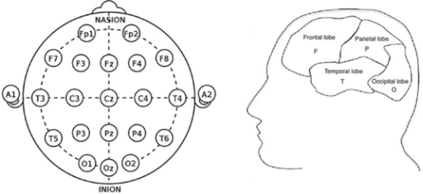
The standardized international 10-20 system is generally used to record EEG activity. This system has 21 electrodes located symmetrically on the surface of the scalp. These positions are computed as percentages of standard distances, the resulting records are comparable between different patients. EEG electrode positions are determined as follows: the reference points are the nasion, which is the delve at the top of the nose, at the level of the eyes; and the inion, which is the bony lump at the base of the skull on the midline at the back of the head. From these points and once the central point (Cz) is localized, the skull perimeters are measured in the transverse and median planes. Electrode locations are determined by dividing these perimeters into 10 % and 20 % intervals, see Fig. 11.1. Additionally, the EEG measurement provides temporal and spatial information about the synchronous firing of many neurons inside the brain with a dominant frequency according to the brain rhythms [1]. The EEG measurement can use a unipolar montage configuration, where the potential of each electrode is compared either to a neutral electrode or to the average of all electrodes; or bipolar montage configuration, where the potential difference between a pair of electrodes spatially close is measured. An artefact in EEG signals is defined as an electrical potential that is not originated in the brain. The two basic artefact types are physiological and non-physiological. A physiological artefact is generated from the electrical activity associated with the patient's body normal functioning, e.g., eye movement and blinking, normal and fast breathing,
Antonio Quintero-Rincón
Department of Electronics, Catholic University of Argentina (UCA), and Epilepsy and Telemetry Integral Center, Foundation for the Fight against Pediatric Neurological Disease (FLENI), Buenos Aires, Argentina.
chewing, bruxism, swallowing, tongue movement, skin potentials, body tremor, cardiac activity, muscle activity, sweat glands, pulse in the tissues, and artificial cardiac pacemaker. A non-physiological artefact is generated by electromagnetic fields outside the body, such as bad signal recording, line frequency (50/60 Hz), misplaced or malfunctioning electrodes, medical equipment, cell phones, lights, and the environmental movement.
Fig. 11.1. Standard 10-20 system montage. Location and nomenclature of the electrodes:
temporal lobe (T), parietal lobe (P), occipital lobe (O), and frontal lobe (F). The odd number corresponds to the left hemisphere and the even number to the right hemisphere.
Noises are as important as artefacts. Acquiring EEG signal properly means mainly measuring biosignals with safety, high signal to noise ratio (SNR) and no data loss. The system electronics include circuitry and printed circuit board design, filtering stages, electronic amplifier’s noise control, correct signal conversion, data storing, contact resistance skin-electrodes, and background noise. See [2-4] for more details.
Significant sources of fluctuating electric potential, proper to the human body, cannot be simply ruled out. They must be filtered out during the EEG measurement. Three examples are the face muscle contractions caused by blinking, the chest motion due to respiration, and the electrocardiogram [5].
Due to the large variability and dynamics of EEG signals, diverse artefacts are common during the acquisition such as sampling errors, noises, unusually small or large values, individual cases that violate the nominal relationship between specific variables, and missing data values. It is very important to know the origins, characteristics, sources, and influence of these anomalies on the data, in order to improve analysis. The goal of this chapter is to review and evaluate some classical methods used to detect different types of EEG artefacts in clinical applications. We review supervised detection methods with a variety of features, including mainly temporal-domain curve fitting, multiple signal frequency-domain, empirical wavelet transforms, t-location-scale statistical modeling, and multivariate analysis with independent vector analysis. Multivariate analysis is widely used to remove artefacts. We show the potential of this approach, using the Hampel filter to correct different types of artefacts. In addition, the chapter provides a complete state-of-the-art along with a recommended bibliography.
11.2. Artefacts
The artefacts caused by involuntary body movements are frequent. They are generated by electrical muscular activity, which can be measured through electromyographic signals (EMG). Muscle contraction, bruxism chewing, swallowing, and tongue movement that include the face, the jaw, and the neck, are examples of EMG. Usually, these types of artefacts occur when the patient is stressed, anxious with difficulties to relax or stay still. To control involuntary movements and correct them, electrodes are placed so that simultaneous reference signals are acquired and correlated with EEG recordings. Involuntary movement can also be controlled using neuromuscular-blocking drugs [6]. For illustration see Figs. 11.2 and 11.3.
Fig. 11.2. Bruxism artefact example. The figure shows that all the channels are affected starting
at 5 seconds abruptly, especially visible between 10 and 20 seconds, and 40 and 45 seconds.
Fig. 11.3. Arm movements artefact example. The figure shows a train of low-amplitude spikes
in all channels starting at 5 seconds, and occasionally high amplitude spikes, as between 5 and 25 sec.
However, depending on the EEG application, muscular artefacts might be highly desired. This is the case in brain-computer interface (BCI) approaches where motor EEG signal imagery is analyzed [7].
Eye movement artefacts, called electrooculogram (EOG), are generated when the eye potential changes between the cornea and the retina. While electroretinogram (ERG) artefacts occur as a response of the eyes-retinal cell to photic stimulation. In general, these artefacts are present in the frontal electrodes such as Fp1, Fp2, F3, F4, and F7, implying many high and low frequencies, depending on their duration and amplitude [6, 8]. ERG artefacts can be corrected by blocking the light source to the eye. Ocular movement can be cancelled by placing a reference electrode over the nose and using a common-mode rejection ratio from a differential amplifier [5].
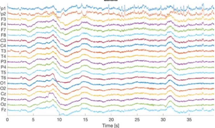
The artefacts produced by the movement of the tongue are called Glossokinetic potential (GKP). These artefacts make the electric field around the mouth and the jaw change as the tongue behaves like a dipole. GKP is best detected in the ramifications located near the mouth, such as the lips, the infraorbital leads, and the Fp1 and Fp2 electrodes. To understand this phenomenon, some tests can be made in order to detect possible artefacts. For example, comparing the not-talk with repeating words that cause significant movement of the tongue, such as saying the expressions “lalala” or “tom thumb”. In children or infants, this artefact is manifested when chewing, sucking, crying, swallowing, or hiccup [6]. See Figs. 11.4 and 11.5 for some examples.
Fig. 11.4. “lalala” artefact example. The figure shows that all channels are affected starting
at 5 seconds, especially from 6 to 15 sec and 30 to 35 sec.
Electrocardiogram (ECG or EKG) artefacts are produced by heart electrical activity. Usually, they have a spike or sharp waveform and can be confused by non-expert with epileptiform activity. The heart rate of the ECG can be recorded by placing two EEG electrodes in any non-cephalic part of the body. The ECG heart rate variability (HRV) can be recorded by placing two EEG electrodes in any non-cephalic part of the body. Due to
their high waveform amplitude, it is possible to distinguish ECG artefacts from natural EEG signals. The voltage of such artefacts is also reduced by using a bipolar instead of a unipolar montage with OA1 and OA2 ear reference electrodes.
Fig. 11.5. Swallowing artefact example. The figure shows high spikes present between 10-sec
and 25-sec on almost all channels.
Power supply (50 or 60 Hz) artefacts are caused by electrical and/or mechanical devices such as the stretcher, ventilation, intravenous infusion devices, sequential compression devices, ECG monitors, dialysis machines, fluorescent lights, heating/cooling, lighting, and rugs. Note that, the 50/60 Hz interference may produce an imprecise reference that can be confused with muscular artefacts or fast brain activity.
This same artefact may be caused by EEG wires in contact with the ground or with electrical wires from other devices, including the power cord from the EEG instrument itself. It can also be caused by poor electrode contact, inadequate preparation of the skin, faulty wiring, or faulty ground making. This artefact leads to high impedance, which can be amplified and detected in one or more channels [9]. In the presence of 50/60 Hz artefacts, and where the impedance of the electrodes is less than 5 KΩ, the plug of each electrical device should be disconnected one at a time while checking the EEG signal improvement. This simple cyclical action permits identifying the source to be removed. At last, a notch filter with a cut-off frequency equal to 50/60 Hz can be used. It must be taken into account that the cerebral signals within this range would also be attenuated. This hinders the detection of epileptiform spikes that have a low amplitude frequency similar to the cut-off frequency [10].
Interruptions between electrodes and the skin can be source of artefacts due to inadequate contact, lack of conductive gel, broken or damaged wires. These are easily distinguished due to the abrupt change in the electrode impedance that creates unexpected potential. Such electrode "pop" may appear in EEG signals as focal spikes or sharp waves with characteristic morphology waveforms having a very steep ascent and a deep fall resembling the shape of the direct current (DC) calibration signal [6]. The movement of
the electrodes can also break their balance that can be identified through the movement magnitude. However, the restoration of the equilibrium point may require a long time, with the possibility of compensation using a low-pass filter with a small cut-off frequency that does not affect the EEG signal [5].
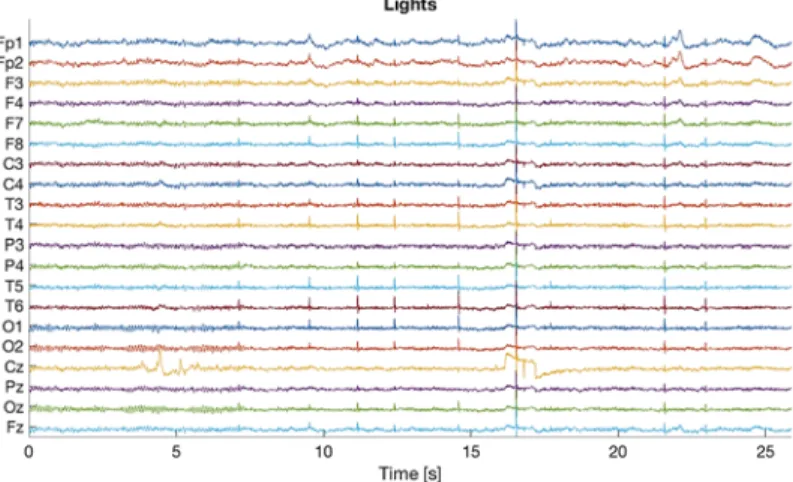
In addition, physical environment factors, such as wires and human movement, can also generate artefacts when they interfere with the magnetic fields. The wires act as antennas and collect different signals by induction, such as power supplies or switching equipment. Human movements near magnetic fields (close to the patient) generate capacitive or electrostatic charges. A controlled environment is required to avoid this type of artefacts. See Figs. 11.6 and 11.7 for some examples.
Fig. 11.6. Example of cell phone artefact. The figure shows an effect
on all channels from 0 to 20 sec.
Fig. 11.7. Example of light artefacts. The figure shows that spike waveforms are exhibited
11.3. Database
For this study, we created a database of EEG signals from two healthy subjects at the Foundation for the Fight against Pediatric Neurological Disease (FLENI) hospital, Buenos Aires. Each signal has 20 unipolar channels with a sampling frequency of 200 Hz, and duration of 1 minute. The location and nomenclature of the electrodes were placed according to the International 10-20 system (Fig. 11.1). Physiological artefacts such as arm and legs movements, swallowing, bruxism, and movement of the tongue with the expression "lalala", were created. While cell phone and light interferences were introduced as non-physiological artefacts. Artefacts were measured successively, with a resting epoch with closed eyes as a control signal after each measurement. Signals measured from the two subjects with 20 channels were partitioned into 1-second segments for subsequent analysis. This resulted in a large dataset with a variety of situations suitable for analysis.
11.4. Artefacts Removal Methods
It is very important that the actions taken to cancel artefacts do not cause new artefacts or loss of neurological valuable information. Therefore, adequate algorithms depend on the intended application. Visual inspection is often required in order to guarantee good signals. This section presents briefly the most common methods used for artefacts cancellation.
Let X NxM the EEG matrix, where M is the number of channels measured
simultaneously. X columns are naturally correlated as electric brain sources are projected on different channels. Assuming, reasonably, that all brain signals arrive at the electrodes instantaneously at the same time, N represents the time-instants of observations
1 2
( ) [ , , , , , ] ,T
m M
x n x x x x (11.1)
We define WK as a moving window so that
,
K K
X W X (11.2)
where K is the positive integer representing the width of the window. Selecting the width is as crucial as the time interval of epochs and segments to capture the phenomenon under study. Typically, in EEG signal processing, the width of 1 or 2 seconds is recommended to guarantee stability, especially with low sampling frequencies [5].
11.4.1. Time-domain Analysis
Empirically, artefacts are determined by using an amplitude threshold. Thus, any signal-segment that crosses the threshold is considered an artefact. Since this is an insufficient condition, some criteria related to the data are usually added. A typical criterion is to combine the threshold with the boundary conditions of the algorithm [11]. For example,
a signal-segment is considered an artefact when the instantaneous amplitude exceeds six times the average amplitude of the recording over the preceding 10 seconds [5].
Usually, the electrical signals generated by the muscular activity have steeper slopes than the average EEG signal. Therefore, the first and second-order derivatives can be used to measure EEG signal mobility [8]. The methodology of differential registration is used in order to improve spatial resolution. The idea is to analyze the signal amplification and digitization systems independently for each electrode with CMOS technology [12]. The time-resolution can be improved by the feed-forward displacements of an order of 10 ms, on the selected time segment. This is used for applications where an analyzing fast signal change is required, such as detecting epileptic seizures [5].
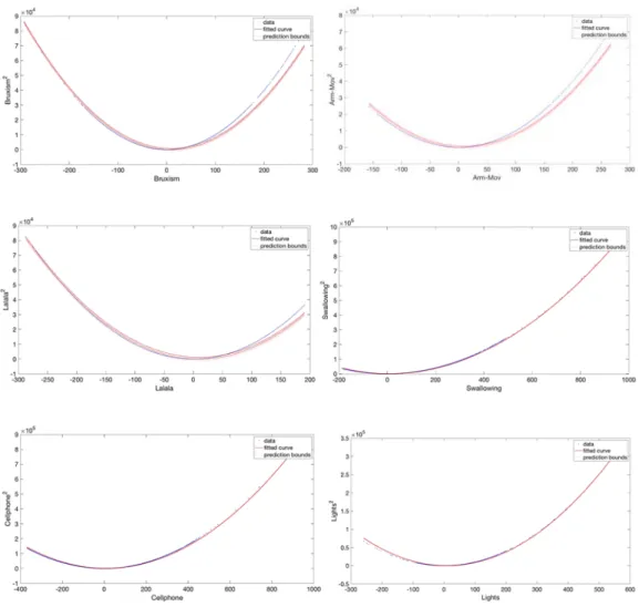
In previous work [13], we found that EEG signals can be analytically represented by using a quadratic linear-parabolic model:
2 sin( ) ( 10)
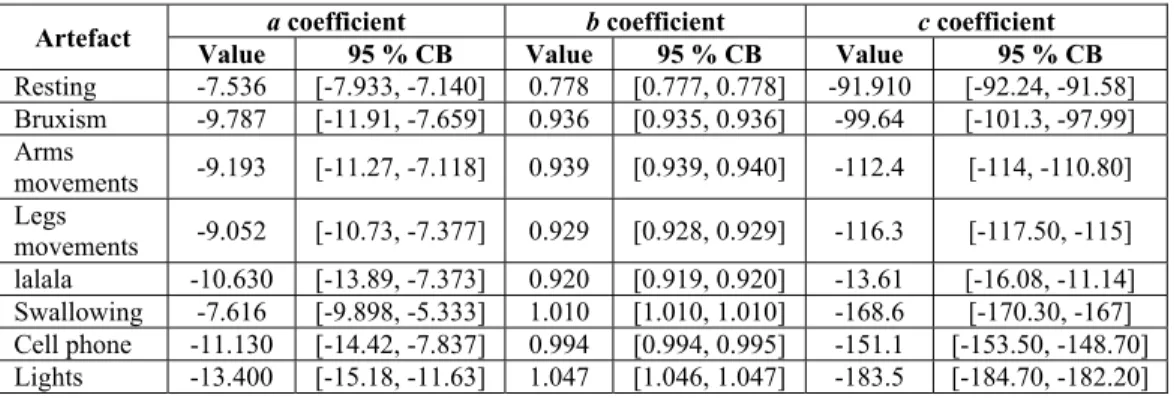
y a x b x . c (11.3) In this work, we make use of this model in order to differentiate EEG resting states signals from artefacts. The underlying hypothesis is that parameters a , b and c are characteristics of these two classes. Here we estimated a, b and c using the least-squares method [14]. Table 11.1 shows the resulting coefficients for different types of signals. One notices that a threshold approach can be used in order to detect artefacts. Figure11.8 illustrates the detection based on this model.
Table 11.1. Estimated quadratic linear-parabolic coefficients and their associated 95%
confidence bounds (CB). These results show that it is possible to use a threshold to distinguish between a resting signal and an artefact.
Artefact Value a coefficient 95 % CB Value b coefficient 95 % CB Value c coefficient 95 % CB
Resting -7.536 [-7.933, -7.140] 0.778 [0.777, 0.778] -91.910 [-92.24, -91.58] Bruxism -9.787 [-11.91, -7.659] 0.936 [0.935, 0.936] -99.64 [-101.3, -97.99] Arms movements -9.193 [-11.27, -7.118] 0.939 [0.939, 0.940] -112.4 [-114, -110.80] Legs movements -9.052 [-10.73, -7.377] 0.929 [0.928, 0.929] -116.3 [-117.50, -115] lalala -10.630 [-13.89, -7.373] 0.920 [0.919, 0.920] -13.61 [-16.08, -11.14] Swallowing -7.616 [-9.898, -5.333] 1.010 [1.010, 1.010] -168.6 [-170.30, -167] Cell phone -11.130 [-14.42, -7.837] 0.994 [0.994, 0.995] -151.1 [-153.50, -148.70] Lights -13.400 [-15.18, -11.63] 1.047 [1.046, 1.047] -183.5 [-184.70, -182.20]
This time-domain experimentation with the quadratic linear-parabolic model brings a different approach to artefact detection in EEG signals, as compared to existing techniques. The confidence intervals estimated for the coefficients (eq.11.3) provide a good discrimination between resting and artefact signals. This simple model can be implemented easily in real-time.
Fig. 11.8. Examples of fitting the quadratic linear-parabolic
model to different artefact signals.
11.4.2. Frequency-domain analysis
Fast Fourier transform (FFT) is the principal linear time-invariant (LTI) method to use with the signal power spectrum density (PSD), PSD x f( ) .2 This is easily achieved by calculating the discrete Fourier transform (DFT) from the correlation function [15]. For example, PSD shows irregular patterns on the higher harmonics of the frequency spectrum for artefacts [8]. PSD can also be used to decompose the EEG signal into different brain rhythms, following current medical practices. It is well known that a large time-interval for the frequency transformation gives a better frequency-resolution [11].
In general, LTI filters are used to reduce EMG and line interference artefacts [16, 17]. Notch and band-pass filters are two classical filters. A notch adaptive digital filter allows
all frequencies to pass except for interference noise [18]. While a band-pass filter is used to filter the low frequencies caused by the muscular activity and the high frequencies generated by medical instrument interferences [5]. This allows attenuating a specific range of frequencies to extract the EEG signal in the purest possible form. The main filtering disadvantage is when an interesting neurological phenomenon occurs, and artefacts are overlapping or in the same frequency band.
11.4.2.1. Singular Value Decomposition (SVD)
SVD is a linear algebra operation that reduces a given matrix to the product of three matrices. Thus, the EEG matrix X NxM can be decomposed as the product of three
matricesXT USVT, where UMxN is an orthonormal matrix obtained from matrix NxN
V , which contains the eigenvectors. SMxN is the diagonal matrix related to the
actual covariance matrix of the data set. The diagonal elements are the singular values representing the variance of the principal components ordered by order of magnitude. The classical expression is given by
0 X v v X v I v X I v (11.3)where
are the square roots of the eigenvalue associated with the variance eigenvector The eigenvectors have the same order as the eigenvalues and should be normalized and scaled by their respective singular values given by the square root of the eigenvalues, to become the principal components with decreasing order of magnitude. Note that, Sand V depend on the source.
11.4.2.2. Multiple Signal Classification (MUSIC)
MUSIC is based on the Pisarenko harmonic decomposition method used to estimate the spectrum of the noise subspace, not the signal subspace. The idea is based on the assumption that after eigenvalue decomposition using SVD for example, the signal and noise subspaces are orthogonal, with a small noise spectrum at frequencies where a signal is present [15]. MUSIC narrowband estimator from the PSD is given by
2 1 1 ( ) , / M k k k p PSD FFT V
(11.4)where M is related to the dimension of the eigenvector, p is the dimension of the signal subspace. Note that, 1 signal subspace p , and p 1 noise subspaceM. kis the
eigenvalue of the thk eigenvector, V is the thk k eigenvector estimated from the correlation matrix of the input signal, which is ordered from the highest to the lowest power, see SVD for more details. Note that the denominator term k is the summation of the scaled power spectra of noise subspace components. If the number of narrowband processes is known, then the dimensions of the signal subspace can be estimated as twice the number of present sinusoids or narrowband processes. If it is unknown, the signal subspace can be determined using the size of the eigenvalues. The idea is based on the fact that the noise components have about the same energy with a flat slope, and the signal components decrease in energy as they are ordered by the energy level. Using a scree plot, it is possible to find the number of components where the eigenvalue plot switches from a downslope to a relatively flat slope.
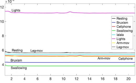
Fig. 11.9 shows the MUSIC performance to detect the different artefacts in EEG signals through the narrowband estimator from its PSD. The resting signal (black color) and legs movements artefacts (gray color) have the same PSD, therefore it is difficult to distinguish them. To the contrary, comparing the resting signal (black color) with the other artefacts, one can clearly see the possibility of distinguishing them using a threshold. Note that, the arm movements artefact (yellow color) and cell phone artefact (yellow color) have similar PSD. However, they are very different from the resting signal. Another interesting threshold is between the resting signal (black color) and the light artefact (magenta color), which has a larger amplitude with respect to the control signal. In physiological artefacts, it is also interesting to note that the resting state has the greatest amplitude with respect to the artefacts. This interesting result is useful in brain-computer interfaces (BCI) and neuron mirror studies with mu rhythm suppression [19]. The mean value and the confidence bounds show in Table 11.2 corroborate these results.
Fig. 11.9. Examples of artefacts using MUSIC narrowband estimator from the PSD. A threshold
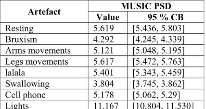
Table 11.2. Values associated with 95 % confidence bounds (CB) from the MUSIC narrowband
estimator from Fig. 11.9. All values are multiplied by e-05.
Artefact Value MUSIC PSD 95 % CB
Resting 5.619 [5.436, 5.803] Bruxism 4.292 [4.245, 4.339] Arms movements 5.121 [5.048, 5.195] Legs movements 5.617 [5.472, 5.763] lalala 5.401 [5.343, 5.459] Swallowing 3.804 [3.745, 3.862] Cell phone 5.178 [5.062, 5.29] Lights 11.167 [10.804, 11.530] 11.4.3. Wavelet-domain Analysis
Many applications rely on the detection and recognition of waveform patterns from the background noise signal. Such waveforms, with spike or wave shapes, are typical in EEG signals. They manifest randomly in a short period of time, and due to their fast transient change, the Fourier analysis does not allow their detection. Therefore, mother wavelet with specific waveform can be used to help detecting such patterns, while determining the exact time at which they occur.
Wavelets used as filter banks analysis are very appropriate for denoising and filtering EEG signals. Typically, the low scales that are related to the high frequencies identify the additive noise. Thus, the signal can be filtered by removing the low-scale components. The next section introduces the 2D empirical Littlewood-Paley wavelet transform as a tool for artefacts detection in EEG signals. The method is based on detecting the Fourier boundaries with an empirical number of filters.
11.4.3.1. 2D Empirical Littlewood-Paley Wavelet Transform
The idea of the empirical wavelet transform (EWT) is to build a family of wavelets adapted to the signal of interest across two steps: 1) Detecting the Fourier supports and building the corresponding wavelet, 2) Filtering the input signal with the obtained filter bank to extract the different components [20].
The 2D empirical Littlewood-Paley transform ( ) is widely used to filter images with 2D
wavelets defined in the Fourier domain on annuli supports, centered around the origin. The inner and outer radius of these supports are fixed upon a dyadic decomposition of the Fourier plane [20]. The wavelets come from the iteration of filters with scaling, with the scale being the inverse of the frequency. Thus, wavelets are obtained from a single prototype mother wavelet by rescaling and shifting. The idea is to use the EEG signal with its rows and columns like a 2D signal as if it was an image [21]. In order to detect the radius of each annuli, the Fourier plane is considered as a polar representation F since P
finding such boundaries is equivalent to working with the frequency modulus . To avoid discontinuities in the output components, the spectrum F is averaged with P
respect to each angle , see equation (11.5) where N is the number of discrete angles. The set of the spectral radius
0, , , n n N with 0 0
and N , is obtained by estimating the Fourier boundaries on FP
.The following 2D empirical Littlewood-Paley wavelet transform algorithm [20] is used: 1. Input: EEG signal f x( )x n( ), number of filters .N
2. Compute the pseudo-polar FFT, F fP
,
and take the average with respect to the angle :
1
01
,
,
N P P i iF
F f
N
(11.5)3. Perform the detection of the Fourier boundaries on FP
to get and build thecorresponding filter bank
1
1
1 , n Nn X X according to
2 1 1 1 1 1 1 1 if 1 1 cos 1 if 1 1 , 2 2 0 otherwise F (11.6) if n N 1:
n n 1 n 1 n 1 n 1 1 2 1 n n n 1 if 1 1 1 cos 1 if 1 1 2 2 1 sin 1 if 1 1 2 2 0 otherwise n N n F
, (11.7) if n N 1:
1 1 1 1 2 1 1 1 if 1 1 sin 1 if 1 1 2 2 0 otherwise,
N N N N N N F
(11.8) 4. Filter f by using equations (11.9) and (11.10)
*
2 2 2 , , f n W n x F F f F (11.9)
*
2 2 2 1 0, , f W x F F f F (11.10)where F is the 2D Fourier transform and 2 * 2
F its inverse.
5. Output:
and Wf
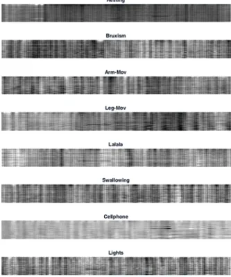
x n, .Figure 11.10 illustrates the 2D empirical Littlewood-Paley wavelet transform reconstruction of a signal by using this algorithm. Through visual inspection, we note that the resting signal has all the components while the other signals are outliers or artefacts.
Fig. 11.10. Signal reconstruction using 2D empirical Littlewood-Paley wavelet transform. The
Fig. 11.11. Concentric boundaries from the 2D empirical Littlewood-Paley wavelet transform. Table 11.3. Mean and bounds of boundaries from 2D empirical Littlewood-Paley wavelet
transform.
Artefact Value Boundaries 95 % BC
Resting 1.924 [0.662, 2.822] Bruxism 1.810 [0.552, 2.810] Arms movements 2.169 [0.154, 2.810] Legs movements 1.679 [0.294, 2.810] lalala 1.983 [0.576, 2.785] Swallowing 1.781 [0.576, 2.773] Cell phone 1.740 [0.564, 2.785] Lights 1.936 [0.589, 2.736]
We propose to use the boundaries of this 2D empirical Littlewood-Paley wavelet transform in order to detect the artefacts in EEG signals. The boundaries estimated using the algorithm introduced above allows us to define a threshold that detects artefacts. Figure 11.11 illustrates the polar representation for the 2D empirical Littlewood-Paley wavelet transform. We can observe the concentric boundary variations. But the visual inspection is complex due to the dynamics and variability of the EEG signals. Table 11.3
shows the mean value, and the confidence bounds of each signal. We can derive a threshold to detect artefacts.
11.4.4. Statistical Modeling
Creating an appropriate parametric statistical model to represent EEG signals can be very useful to capture the characteristics of the underlying physical process. When feasible, this is often done by fitting a statistical distribution to data histograms. In previous works, we found that the t-location-scale distribution is powerful for modeling EEG signals [22-24]. Fitting this distribution was performed by estimating its three parameters, namely location, scale, and shape, using maximum likelihood estimators. In this section, we use this distribution in order to characterize and detect artefacts.
11.4.4.1. The t-location-scale Distribution
The t-location-scale distribution is a statistical model that belongs to the location-scale family formed by translation and rescaling of the Student’s t-distribution. Its probability density function (PDF) is given by
1 2 2 1 2 | , , , 2 x f x (11.11)where is the location parameter, is the scale parameter, 0 is the 0 shape parameter, and (.) is the Gamma function. Figure 11.12 shows the fit of the distribution to our EEG data histograms. This shows a good fit and makes it possible to correctly characterize different artefacts the distribution parameters.
From Table 11.4, one notices that it is possible to discriminate artefacts from a resting signal. The scale and shape parameters can be used in a straightforward manner to discriminate between artefacts and non-artefacts. While values of the location parameter associated with a muscular artefact and resting signal are close. Nevertheless, discrimination is still possible.
11.4.5. Multivariate Analysis
The principle of multivariate analysis is to consider the relationship between multiple variables. Precisely, this analysis operates on all data or measurements but treats them as a single entity.
Fig. 11.12. Fits of the t-location-scale distribution to histograms of data for different artefacts. Table 11.4. Mean values associated with 95 % confidence bounds (CB) from the t-location-scale
parameters. These results show that it is possible to use intervals to differentiate between normal (resting) signals and artefacts.
Artefact Value Location parameter 95 % CB Value Scale parameter 95 % CB Value Shape parameter 95 % CB Resting -3.243 [-3.258, -3.229] 9.763 [9.749, 9.777] 6.598 [6.553, 6.644] Bruxism -3.580 [-3.631, -3.529] 14.257 [14.199, 14.316] 2.197 [2.179, 2.215] Arm movements -3.205 [-3.257, -3.153] 13.351 [13.293,13.410] 2.349 [2.328, 2.370] Legs movements -3.220 [-3.266, -3.174] 12.444 [12.396, 12.493] 2.958 [2.929, 2.987] lalala -3.747 [-3.819,-3.676] 17.309 [17.219, 17.400] 1.653 [1.639, 1.666] Swallowing -2.789 [-2.837, -2.740] 14.123 [14.069, 14.177] 2.069 [2.054, 2.084] Cell phone -4.513 [-4.565, -4.462] 1.677 [1.666, 1.689] 1.677 [1.666, 1.689] Lights -4.203 [-4.250, -4.155] 3.733 [3.674, 3.793] 3.733 [3.674, 3.793]
A classic example is the covariance matrix that incorporates variance related to the individual variables, and the covariance between variables. In essence, the multivariate data transformations search for a dimensional reduction. Three multivariate techniques used for this purpose are principal component analysis (PCA), independent component analysis (ICA), and independent vector analysis (IVA), all based on blind source separation (BSS). These techniques will be presented below in the context of EEG processing.
11.4.5.1. Blind Source Separation (BSS)
BSS assumes that the source signals reach the electrodes at the same time t instantaneously, equation (11.1) can be reformulated as
( ) ( ) ( ),
x n H s n v n (11.12)
where x n( ) is the EEG matrix, H is the mixing matrix, s n( ) is the matrix of the sources, and v n( ) is the noise. The separation is carried out by means of the matrix W , which uses only the information about x n( ) to reconstruct the original source signals as:
( ) ( )
y n W x n (11.13)
In BBS, the goal is to estimate the unmixing matrix W by using the singular value decomposition method (SVD) such that Y WX best approximates the independent sources ,S where ( )
1( ), , ( )
T M y n y n y n and ( )
1( ), , ( ) ,
T M x n x n x n therefore , S Y WX see Fig. 11.13.Fig. 11.13. Illustration of mixing information from brain sources s n( ) to create an EEG channel
( ).
x n Multivariate analysis methods aim at finding the brain sources that generated the EEG signals (source [29]).
During the BSS process, the method separates EEG signals into components of the EEG signals. Components attributed to artefacts are identified and discarded. The signal is then reconstructed based only on the remaining components. This method does not require having the reference of artefacts. BBS is typically used to correct EOG, EMG, and ECG signals [25-27].
11.4.5.2. Principal Component Analysis (PCA)
In PCA the idea is to transform the original data into a new smaller dimension dataset without loss of information. This transformation between a dataset of correlated variables into a new dataset of decorrelate variables is called principal components because it includes the most significant information from the original data. PCA uses the eigenvectors of the covariance matrix from the original data set in order to transform the data into another coordinate system, estimating the input projection data with their higher variability. Once this is done, the data set components are extracted by the eigenvectors data projection, see the previous two sections for more details. In the PCA algorithm, three recommendations have to be considered: i) data must be centered by removing the mean values
x x
., ii) data must be rotated in order to decorrelate it, iii) the data must be normalized according to its variance before the transformation. The normalization process removes variables with very small values. For example, if 12, the information energy will be mostly concentrated in the dominant matrix X1 1 1 1u v associated with the first singular values. This will be higher with respect to the other values; therefore, many values could be removed. According to [28], PCA cannot completely separate eye-movement artefacts, EMG, and ECG artefacts from the EEG signal, especially when they have comparable amplitudes. PCA also does not necessarily decompose similar EEG features into the same components when applied to different segments. Additionally, PCA is not consistent with respect to the interference suppression from overlapping brain activity [30]. One solution is to use the artefact subspace reconstruction (ASR) approach. The idea is to learn from a clean calibration statistical data model in order to attenuate the EEG artefacts by decomposing it in small segments and comparing them to calibration data in the PCA component subspaces [31]. A recent interesting study was done in simultaneous EEG-fMRI data, where the helium-pump artefacts given by the mechanical vibrations in the MRI system were removed using the EEG-segment-based principal component analysis in the gamma band [32].11.4.5.3. Independent Component Analysis (ICA)
In PCA, the data decorrelation is not sufficient to produce independence between the variables at least when the variables have non-Gaussian distributions [15]. Thus, the ICA goal is to transform the original data into statistically independent variables, which will be the most significant variables. The assumption is that the original variables are independent and non-Gaussian. The signals are assumed to be linear combinations of these original variables, with negligible propagation delay.
As such, the EEG signals are considered as combinations of the underlying neural sources with added artefacts. Signals from multiple sources S are assumed to arrive simultaneously at electrodes X see Fig. 11.8. The number of sources is usually greater than the number of electrodes. Each electrode consists of a mixture of all sources, which are assumed independent. Therefore, applying ICA to EEG signals is a way for estimating the sources. The goal is not to reduce the number of signals, but to produce signals that are more meaningful. The typical model that relates the sources with the measurements is given by
,
x As (11.14)
where x vector of EEG signals, s are the sources, and A is the mixing matrix. This assumes that the measured signal vector x, is related to the underlying source signals vector s by a linear transformation. The objective is to determine the unknown mixing matrix. Assuming that the mixing matrix is square, the independent components can be obtained through matrix inversion
1 ,
s A x (11.15)
Since the size of x is supposed to be higher than s , inversion cannot be done immediately. PCA is usually applied first to reduce the number of components to be equal to the considered number of sources. Then the ICA algorithm is applied. While assuming sources to be independent and non-Gaussian, this method does not require their distribution to be known [15]. The following standard ICA algorithm is used:
ICA algorithm
1. Center the original data by removing the mean values
x x
. Note that, the signals are assumed to be correlated.2. Apply a whitening process by rotating the data in order to decorrelate them until the non-Gaussianity of the transformed data set is maximized. This process helps to trace variance information. After whitening, the components must be scaled in order to have unit variance
21.3. Estimate the data Gaussianity. The estimation builds on the result of the central limit theorem that states that the distribution of a set of k random variables that are independent and identically distributed with mean and variance 02 1, converges to a Gaussian distribution as k grows, regardless of the distribution of the independent variables. The kurtosis measurement is used to quantify the lack of data Gaussianity. Kurtosis is the fourth order cumulant defined as
24 2
( ) 3 ,
kurt x E x E x where E is the expectation operator. Kurtosis may compress the data using a nonlinear function to restrain outliers before taking the fourth power [15]. Note that, for real data that have zero mean, the variance E x
2
2, therefore kurt x( ) mean( ) 3. x4 Depending on the shape of the distribution, there are three types of denominations. If kurt one speaks about non-Gaussian distribution, 0if kurt that data has sub-Gaussian distribution with shape broad and flat, and if 0 0
kurt data has super-Gaussian distribution with shape spiky. 4. Estimate eigenvalues of x.
5. Apply JADE algorithm for a real-valued signal [33] to find the unmixing matrix A1 with the number of independent components.
EEG signals have the assumption that the volume conduction is linear and instantaneous and the underlying brain signals are mixed together with their artefacts. Thus, the eye and muscular activity sources, line noise, and cardiac signal usually are not separated from the EEG sources activity. Therefore, ICA assumes that there exists an effective number of statistically independent signals that contribute to the scalp activity and that are not known. But it is possible to find them and discriminate between the artefacts when the signal is reconstructed using the unmixing signal, see equation (11.14) and equation (11.15). ICA was adopted as a strong algorithm used within the EEGLAB toolbox for eliminating multiple artefacts [34] and continues to evolve with the help of the scientific community as will be exposed by using the independent vector analysis approach in the next subsection.
11.4.5.4. Independent vector analysis (IVA)
IVA is an extension from the univariate source signals formulation to multivariate source signals formulation [35]. We use the algorithm proposed in [36], where the idea is to minimize the BSS mutual information through the sources to achieve independent vector analysis with second-order statistical information across datasets by assuming that the source component vector distributions are multivariate Gaussians. Precisely, this type of assumption has been considered in EEG signals [21, 37]. In [36], the proposed approach has the particularity of relying on a cost function equivalent to a particular multiset canonical correlation analysis (MCCA). Thus, the IVA cost function minimization by using a decoupled gradient-based optimization scheme permits us to find the set of nonorthogonal unmixing matrices.
Let us consider the multivariate formulation based on the classical BBS approach problem, see equation (11.12), for data observations from K datasets each formed from linear mixtures of N independent sources
[ ]K [ ] [ ]K K , 1 , X A s k K (11.16) where [ ] [ ] [ ] 1 , , T K k k N
s s s is the zero-mean source vector, and
A
[ ]K is the invertible mixing matrixA
[ ]K,
see equation (11.14). They are unknown real-valued quantities to be estimated. The n-th source component vector [1], , [ ]K Tn n n
s s s is independent of all other source component vectors within the dataset and exactly dependent on at most one source in each of the other datasets. Therefore, their joint distribution for all the
independent sources is given by
1
1
, ,
N Nn( ).
np s
s
p s
The BBS approach solution is given byy
[ ]K
W
[ ] [ ]Kx
K,
where the goal is to find K unmixing matrices[ ]K
W
and source vector estimates for each datasety
[ ]K,
see equation (11.13).
The identification of the independent source component vectors is achieved by minimizing the mutual information among the source component vectors
[ ] 1 1 1 [ ] [ ] 1 1 1 1 log det log det , N K k IVA N n k N K K k k N N n k k H y W C H y I y W C
I (11.17) where [1], , [ ]K T N n ny y y is the n-th source component vector estimation
s
n, and1
C
denotes the constant term [1], , [ ]K .H x x The equation (11.17) shows that minimizing the cost function simultaneously minimizes the entropy of all components and maximizes the mutual information within each source component vector.
The zero-mean and real-valued multivariate Gaussian distribution is useful to solve the joint BSS approach problem using second-order statistics and is given by
1 1 2 2 1 1 | exp , 2 2 det T n n K n n n n p y y y
(11.18)where K is the source component vector dimension and is the covariance matrix. Substituting in the equation (11.17) the expression
1
1
log 2
,
2
K K k kH y
e
where k is the -thk eigenvalue of the covariance matrix . Then, the cost function for the multivariate Gaussian distribution is given by
[ ] , 1 1 1 1log 2
1
log
log det
,
2
2
N K K k IVA MG k k n k nNK
e
W
C
I
(11.18)where k n, is the -thk eigenvalue of the covariance matrix associated with the -thn
source component vector. The cost function from equation (11.18) indicates that the product of the source component vector covariance eigenvalues should be minimized. Under the constraint that the sum of the eigenvalues is fixed, then the minimal cost is met when each covariance matrix is as ill-conditioned as possible. Thus, the eigenvalues are maximally spread apart. See [36] for a general description of this multivariate Gaussian formulation.
In order to check the potentiality of the independent vector analysis (IVA), we use the bruxism signal that has artefacts in all channels, see Fig. 11.2. For illustration, the resulting demixing matrices W[ ]K are illustrated in Fig. 11.14, and the signal reconstruction is
shown in Fig. 11.15. Note that, this process can help to remove artefacts from the signal, as it can be seen in the difference between Fig. 11.2 and Fig. 11.15. However, it is important to make a visual inspection with the expert physician.
Fig. 11.14. Example of unmixing matrices obtained using IVA for Bruxism signals.
Fig. 11.15. Example of reconstructed Bruxism signals using IVA.
11.4.6. Data-mining Domain
Data mining is usually defined as the use of automated procedures to extract useful information and insight from large datasets such as the EEG signal [38]. In practice, the EEG data contains various types of anomalous measurements, which are typical during the signal acquisition. These anomalous measurements can complicate the analysis
because of the prevalence of artefacts, outliers, missing or incomplete data, and other more subtle phenomena such as misalignments. Results that are essential to the medical diagnosis might be invalidated due to these phenomena. We propose the Hampel filter to correct artefacts in EEG signals. This is a non-linear filter for data cleaning that searches outliers or abnormal local data in a temporal sequence, making it interesting for looking for abnormalities in EEG signals. The motivation of using this filter is related to a previous no published work [39] where a descriptive statistical analysis and visual inspection were used to study the performance of the Hampel filter. This filter has been used in the literature to study physiological signals, as in [40, 41] for removing artefacts in deep brain stimulation (DBS), and in [42] for compensating motion artefacts in ECG signals.
11.4.6.1. Hampel Filter
Let Kin the equation (11.1) be the positive tuning integer flexible parameter from the window half-width WK. The standard median filter
k
m
using the moving data window for each channel sequence
X
k is given by
median
, , , ,
,
k k K k k K
m
x
x
x
(11.19)The main advantage of the median is its extreme resistance to local outliers or impulsive noise. While its main disadvantage is the possible introduction of significant distortions. The Hampel filter
H
K belongs to the class of decision-based filters [38] that detect outliers based on the median and the MAD scale estimator. It is based on the moving-window implementation of the Hampel identifier [43]. The filter response is given by,
k k k k k k k k kx x
m
tS
y
m x
m
tS
(11.20)where
m
k is the median value from the moving data window andS
k is the MAD scale estimate, defined by ,
1.4826 median
k j K K k j k
S x m . (11.21)
The factor S allows the MAD scale estimator of the standard deviation of Gaussian data to be unbiased. Precisely, EEG signals have been shown to follow a generalized Gaussian distribution [37]. Consequently, the Hampel filter is a good candidate to cancel outliers and artefacts in EEG. Note that if the threshold parameter t0, the standard median filter corresponds to yK t| 0 mk. This allows using the Hampel filter as a generalization of the median filter, with t as an additional tuning parameter. Note that the MAD scale estimator
is sensitive to implosion. If more than 50 % of the data values are the same, the MAD scale estimate is zero, independently of the other values and the parameter .t Thus, data
must implosion-free in order to obtain a correct characterization of the signal. Then, for an implosion-free sequence
xk , the Hampel filter reduces to an identity filter for some sufficiently large but finite value of t restricted to the range 0 t T, where T is the threshold value. Thus,max
min
k k k k kx
m
t
S
(11.22)We refer the reader to [43, 38, 44] for a comprehensive treatment of the mathematical properties of the Hampel filter.
In order to evaluate this filter, we run experiments on short epochs from each artefact signals. These epochs were annotated by a neurologist to indicate the location of the artefact in the signal. Figure 11.16 shows the results. We can notice that for physiological artefacts, when the variability of the EEG signal to that of the artefact, the Hampel filter corrections are close to the original signal. However, with high peaks, the filter brings over-corrections. We, therefore, recommend choosing a correct moving window in order to not lose relevant information. Inversely, for non-physiological artefacts, the high peaks are the principal outliers to correct making the Hampel filter useful for this type of outliers. However, visual inspection remains essential to avoid losing relevant information.
11.5. Conclusions
In this chapter, we reviewed some classical signal processing methods for detecting and removing artefacts in EEG signals. The goal was to use a supervised analysis to estimate a threshold capable of discriminating between normal EEG and artefact signals. Experiments were conducted using a signal database created specifically for this purpose. A resting-state signal was used as a control signal for comparing with artefact signals of different types. First, a time-domain analysis was used to detect artefacts with a linear-parabolic model-fitting method. Results showed that the linear-parabolic waveform is interesting in analyzing EEG signals with a convex waveform. Second, the MUSIC algorithm was used to conduct frequency-domain analysis using a narrowband estimator from the power spectrum density of the signal. Results showed interesting discrimination between normal signals and artefacts, but with a high computational cost. The third review was with wavelet-domain analysis, where we evaluated the 2D empirical Littlewood-Paley wavelet transform across its boundaries. Using boundaries as features turned out to be useful to differentiate between normal and artefact signals. Finally, the study of the statistical parameters of the t-location-scale distribution showed a good fit with EEG data. Using these parameters as features were shown to be useful for detecting artefacts in EEG signals. In conclusion, the study of all these methods showed the feasibility of detecting artefacts in EEG signals, with good performance. This makes possible the design a multi-class or multi-label detection-multi-classification [45] with unbalanced data [46], which is would be very useful during the acquisition of EEG signals.
Fig. 11.16. Examples of artefact epochs extracted from one EEG channel. The blue line is
the original signal, and the red line is the signal with the outliers removed using the Hampel filter.
For artefacts removal, we evaluated the IVA algorithm from the multivariate analysis domain and the Hampel filter as a data-mining technique. These have proven to be effective techniques to remove outliers and artefacts. Such methods can be implemented in combination with the detection methods described above to achieve automatic detection and filtering processes. However, it is important to conduct such an analysis under the supervision of expert neurologists in order to not lose essential medical information.
References
[1]. J. Malmivuo, R. Plonsey, Bioelectromagnetism, Oxford University Press, 1995.
[2]. C. M. Sinclair, M. C. Gasper, A. S. Blum, Basic electronics in clinical neurophysiology, The
[3]. S. V. Vaseghi, Advanced Digital Signal Processing and Noise Reduction, Wiley, 2006. [4]. A. B. Usakli, Improvement of EEG signal acquisition: An electrical aspect for state of the art
of front end, Computational Intelligence and Neuroscience, Vol. 2010, 2010, 630649. [5]. K. Najarian, R. Splinter, Biomedical Signal and Image Processing, CRC Press, 2016. [6]. D. M. White, C. A. Van Cott, EEG artefacts in the intensive care unit setting, American
Journal of Electroneurodiagnostic Technology, Vol. 50, Issue 1, 2010, pp. 8-25.
[8]. L. Sörnmo, P. Laguna, Bioelectrical Signal Processing in Cardiac and Neurological Applications, Academic Press, 2005.
[7]. L. Frølich, I. Winkler, K.-R. Müller, Investigating effects of different artefact types on motor imagery BCI, in Proceedings of the 37th Annual International Conference of the IEEE Engineering in Medicine and Biology Society (EMBC’15), 2015, pp. 1942-1945.
[9]. A. Peper, C. A. Grimbergen, EEG measurement during electrical stimulation, IEEE
Transactions on Biomedical Engineering, Vol. 30, Issue 4, 1983, pp. 231-233.
[10]. S. Sanei, J. A. Chambers, EEG Signal Processing, Wiley-Interscience, 2013. [11]. W. van Drongelen, Signal Processing for Neuroscientists, Academic Press, 2018.
[12]. S.-F. Yen, D. Schoonover, J. C. Sanchez, J. C. Principe, J. G. Harris, Differential EEG, in
Proceedings of the 4th International IEEE/EMBS Conference on Neural Engineering
(NER’09), 2009, pp. 18-21.
[13]. A. Quintero-Rincón, C. D'Giano, H. Batatia, A quadratic linear-parabolic model-based EEG classification to detect epileptic seizures, The Journal of Biomedical Research, Vol. 34, Issue 3, pp. 205-212, 2020.
[14]. P. C. Hansen, V. Pereyra, G. Scherer, Least Squares Data Fitting with Applications, Johns
Hopkins University Press, 2013.
[15]. J. L. Semmlow, Benjamin Griffel, Biosignal and Medical Image Processing, CRC Press, 2014.
[16]. L. P. Panych, J. A. Wada, M. P. Beddoes, Practical digital filters for reducing EMG artefact in EEG seizure recording, Electroencephalography and Clinical Neurophysiology, Vol. 72, Issue 3, 1989, pp. 268-276.
[17]. M. van de Velde, G. van Erp, P. J. Cluitmans, Detection of muscle artefact in the normal human awake EEG, Electroencephalography and Clinical Neurophysiology, Vol. 107, Issue 2, 1998, pp. 149-158.
[18]. S. P. Cho, M. H. Song, Y. C. P. Choi, H. Seon, K. J. Lee, Adaptive noise canceling of electrocardiogram artefacts in single channel electroencephalogram, in Proceedings of the
29th Annual International Conference of the IEEE Engineering in Medicine and Biology
Society (EMBS’07), 2007, pp. 3278-3281.
[19]. A. Quintero-Rincón, C. D'Giano, H. Batatia, Mu-suppression detection in motor imagery electroencephalographic signals using the generalized extreme value distribution, in
Proceedings of the International Joint Conference on Neural Networks (IJCNN’ 2020), 2020,
pp. 1-5.
[20]. J. Gilles, G. Tran, S. Osher, 2D Empirical transforms. Wavelets, ridgelets and curvelets revisited, SIAM Journal on Imaging Sciences, Vol. 7, Issue 1, 2014, pp. 157-186.
[21]. A. Quintero-Rincón, J. Prendes, M. A. Pereyra, H. Batatia, M. Risk, Multivariate Bayesian classification of epilepsy EEG signals, in Proceedings of the 12th IEEE Workshop on Image,
Video, and Multidimensional Signal Processing (IVMSP’16), 2016, pp. 1-5.
[22]. A. Quintero-Rincón, J. Prendes, V. Muro, C. D'Giano, Study on spike-and-wave detection in epileptic signals using t-location-scale distribution and the k-nearest neighbors classifier, in
Proceedings of the IEEE URUCON Congress on Electronics, Electrical Engineering and Computing, 2017, pp. 1-4.
[23]. I. Zorgno, et al., Epilepsy seizure onset detection applying 1-NN classifier based on statistical parameters, in Proceedings of the Biennial Congress of Argentina (ARGENCON’18), 2018, pp. 1-5.
[24]. A. Quintero-Rincón, V. Muro, C. D’Giano, J. Prendes, H. Batatia, Statistical Model-Based Classification to Detect Patient-Specific Spike-and-Wave, Computers, Vol. 9, Issue 4, 2020, pp. 1-14.
[25]. L. Shoker, S. Sanei, M. A. Latif, Removal of eye blinking artefacts from EEG incorporating a new constrained BSS algorithm, in Proceedings of the Annual International Conference of
the IEEE Engineering in Medicine and Biology Society (EMBS’04), 2004, pp. 909-912.
[26]. J. Gao, P. Lin, P. Wang, Y. Yang, Online EMG artefacts removal from EEG based on blind source separation, in Proceedings of the 2nd International Asia Conference on Informatics in
Control, Automation and Robotics (ICINCO’10), 2010, pp. 28-31.
[27]. H. Hallez, A. Vergult, R. Phlypo, I. Lemahieu, Muscle and eye movement artefact removal prior to EEG source localization, in Proceedings of the Annual International Conference of
the IEEE Engineering in Medicine and Biology Society (EMBS’06), 2006, pp. 1002-1005.
[28]. G. Geetha, S. N. Geethalakshmi, Scrutinizing different techniques for artefact removal from EEG signals, International Journal of Engineering Science and Technology (IJEST), Vol. 3, Issue 2, 2011, pp. 1167-1172.
[29]. A. Quintero-Rincón, M. Flugelman, J. Prendes, C. D'Giano, Study on epileptic seizure detection in EEG signals using largest Lyapunov exponents and logistic regression, Revista
Argentina de Bioingeniería, Vol. 23, Issue 2, 2019, pp. 17-24.
[30]. N. T. Haumann, M. Huotilainen, P. Vuust, E. Brattico, Applying stochastic spike train theory for high-accuracy human MEG/EEG, Journal of Neuroscience Methods, Vol. 340, 2020, 108743.
[31]. T. R. Mullen, et al., Real-time neuroimaging and cognitive monitoring using wearable dry EEG, IEEE Transactions on Biomedical Engineering, Vol. 62, Issue 11, 2015, pp. 2553-2567. [32]. H.C. Kim, S.-S. Yoo, J.-H. Lee, Recursive approach of EEG-segment-based principal component analysis substantially reduces cryogenic pump artefacts in simultaneous EEG-fMRI data, Neuroimage, Vol. 104, 2015, pp. 437-451.
[33]. J. F. Cardoso, A. Souloumiac, Blind beamforming for non-Gaussian signals, IEE Proceedings
F – Radar and Signal Processing, Vol. 140, Issue 6, 1993, pp. 362-370.
[34]. D. Arnaud, S. Makeig, EEGLAB: An open source toolbox for analysis of single-trial EEG dynamics including independent component analysis, Journal of Neuroscience Methods, Vol. 134, 2004, pp. 9-21.
[35]. T. Kim, I. Lee, T.-W. Lee, Independent vector analysis: Definition and algorithms, in
Proceedings of the Fortieth Asilomar Conference on Signals, Systems and Computers (ACSSC’06), 2006, pp. 1393-1396.
[36]. M. Anderson, X.L. Li, T. Adali, Nonorthogonal independent vector analysis using multivariate Gaussian model, Lecture Notes in Computer Science, Vol. 6365, 2010, pp. 354-361.
[37]. A. Quintero-Rincón, M. Pereyra, C. Risk, M. D'Giano, H. Batatia, Fast statistical model-based classification of epileptic EEG signals, Biocybernetics and Biomedical Engineering, Vol. 38, 2018, pp. 877-889.
[38]. R.K. Pearson, Mining Imperfect Data Dealing with Contamination and Incomplete Records, SIAM: Society for Industrial and Applied Mathematics, 2005.
[39]. A. Quintero-Rincón, M. Risk, S. Liberczuk, EEG preprocessing with Hampel filters, in
Proceedings of the Biennial Congress of Argentina (ARGENCON’12), Vol. 89, 2012,
pp. 1-6.
[40]. M. Dagar, N. Mishra, A. Rani, S. Agarwal, J. Yadav, Performance comparison of Hampel and median filters in removing deep brain stimulation artefact, Innovations in Computational
Intelligence, Studies in Computational Intelligence, Vol. 713, 2018, pp. 17-28.
[41]. D. P. Allen, E. L. Stegemöller, C. Zadikoff, J. M. Rosenow, C. D. Mackinnon, Suppression of deep brain stimulation artefacts from the electroencephalogram by frequency-domain Hampel filtering, Clinical Neurophysiology, Vol. 121, Issue 8, pp. 1227-1232, 2010.
[42]. F. A. Ghaleb, M. B. Kamat, M. Salleh, M. F. Rohani, S. A. Razak, Two-stage motion artefact reduction algorithm for electrocardiogram using weighted adaptive noise cancelling and recursive Hampel filter, PLoS ONE, Vol. 13, Issue 11, 2018, e0207176.
[43]. A. Davies, U. Gather, The identification of multiple outliers, Journal of the American
Statistical Association, Vol. 88, Issue 423, 1993, pp. 782-792.
[44]. R. K. Pearson, Y. Neuvo, J. Astola, M. Gabbouj, Generalized Hampel filters, EURASIP
Journal on Advances in Signal, 2016, 87.
[45]. F. Herrera, F. Charte, A. J. Rivera, M. J. del Jesus, Multilabel Classification, Springer, 2016. [46]. A. Fernández, et al., Learning from Imbalanced Data Sets, Springer, 2018.