FACTEURS ÉCOLOGIQUES ET EVOLUTIFS INFLUENÇANT LES DYNAMIQUES D'AIRE DE REPARTITION GÉOGRAPHIQUE DES ESPÈCES
ET LEURS EFFETS SUR LES PATRONS DE BIODIVERSITÉ À LARGE ÉCHELLE
THÈSE PRES ENTÉ
COMME EXIGENCE PARTIELLE DU DOCTORAT EN BIOLOGIE
PAR
RENATO HENRIQUES DA SILVA
Avertissement
La diffusion de cette thèse se fait dans le respect des droits de son auteur, qui a signé le formulaire Autorisation de reproduire et de diffuser un travail de recherche de cycles supérieurs (SDU-522 - Rév.0?-2011 ). Cette autorisation stipule que «conformément à l'article 11 du Règlement no 8 des études de cycles supérieurs, [l'auteur] concède à l'Université du Québec à Montréal une licence non exclusive d'utilisation et de publication de la totalité ou d'une partie importante de [son] travail de recherche pour des fins pédagogiques et non commerciales. Plus précisément, [l'auteur] autorise l'Université du Québec à Montréal à reproduire, diffuser, prêter, distribuer ou vendre des copies de [son] travail de recherche à des fins non commerciales sur quelque support que ce soit, y compris l'Internet. Cette licence et cette autorisation n'entraînent pas une renonciation de [la] part [de l'auteur] à [ses] droits moraux ni à [ses] droits de propriété intellectuelle. Sauf entente contraire, [l'auteur] conserve la liberté de diffuser et de commercialiser ou non ce travail dont [il] possède un exemplaire.»
This has been a long journey that cannot be resumed only by the document presented here, especially since this work was achieved in a completely different country (and Earth hemisphere) from where 1 used to live. lt was not a trivial task to adapt to a new society, with different values and rules, while working on my doctorate. As such, the "human component" he re in Montreal was crucial for my professional (and persona!) achievement. 1 owe this to many people and being thankful costs very little and do lots of good for both the thank:ful and the thanked. The only risk is to forget to name someone that should be named. First, 1 am very grateful to have been supervised by Pedro R. Peres-Neto. He is a passionate scientist with endless ideas that he continuously shared with me and other students while allowing us to choose which one to pursue and how to conduct it. 1 would like to describe our interaction using a modified quote from Joshua Schimel's book Writing Science: "When 1 was a graduate student, 1 would sometimes go to my advisor, Pedro Peres-Neto, with what 1 thought was a simple question. Then we might spend weeks discussing issues that wandered al! over the intellectual map and didn 't appear to fit on the straight raad from my question to the answer. Many of the issues Pedro raised seemed irrelevant and extraneous. Over the years 1 worked with him, 1 came to understand what we were really doing in those conversations. Pedro saw more of the system and how it fit
later. Though not a/ways easy, it was an important lesson, one 1 remain gratefulfor." He was very open to my own ideas and supported my choices throughout this period. Pedro is also a very interesting character on a persona! leve! and I always enjoyed the great discussions we had about politics, cultures, languages, food, society and science among others. I appreciate that he was always honest and direct (sometimes too much) about how he felt of someone or something; in any case, you would always know what he was thinking. Finally I want to say that our interactions were crucial for my success. I have improved in so many ways regarding my academie training during this period and I am sure that this experience will be invaluable after I leave his !ab. I am also deeply thankful to my co-supervisor Bernadette Pinel-Alloul, for her advices and support throughout my doctoral program. Although we did not interact as much, every time I needed sorne advice or help she would ~o so promptly. I also want to thank Ginette Méthot and Lama Aldamman from Bernadette's Lab for their help on zooplankton identification. I am thankful to bath my proposai and comprehensive exam committees: Beatrix Beisner, Steven Kembel, Alison Derry and Patrick James. Their suggestions, insights, critics and questions were invaluable to my improvement as a scientist. I would like to thank the co-authors Vincent Calcagno, Mark C. Urban and Alexander Kubisch for their counselling and insights, and specially my co-author and good friend Frédéric Boivin for countless hours of
remain in contact independently of our future paths. I am very happy to have met Bailey Jacobson, with whom I shared the lab for more than seven years during both my master and PhD programs. I have never met someone as good-hearted, hardworking and responsible as Bailey. I am truly grateful for her support and friendship during all these years and for her patience to correct the English from my manuscripts, especially during my fust years in the lab. I cannat forget about Mehdi Layeghifard, who helped ine a lot during my PhD. He is a very opinionated persan and we always had great discussions. I would also like to acknowledge Jason Samson, who is probably the most positive-thinking persan I've ever met. He helped me through tough times and, as a bonus, taught me a lot about GIS. I am grateful for my past and current lab mates, as well as all the people that came here for internship or sabbatical, for all their support throughout this period; sorne of them have become very good friends: Aline Aguiar, Andrew Smith, Caroline Senay, Daniel Pieres, Emily Tissier, Fernanda Melo Cameiro, Georgina O'Farrill, Haycen Alleg, Hedvig Nénzen, Henrique Giacomini, Hugo Martinez, Ignacio Castilla-Morales, Izaias Fernandes, Joaquim Réné Jacquart, Louis Donelle, Marcia Marques, Marie-Christine Bellemare, Marie-Hélène Greffard, Patricia Rodriguez Gonzalez, Pedro de Podestà, Pedro Henrique Pereira Braga, Richard Vogt, Shubha Pandit, Sylvie Clappe, Vitor Prado, Viviane Monteiro, Wagner Moreira, Will Pearse and Who-Seung Lee. I would
Gabrielle Dubuc Messier, Isabelle Laforest-Lapointe, Juan Pablo Nifio, Jorge Negrin Dastis, Kimberley Lemmen, Laura Redmond, Laurence Puillet, Luc De Meester, Luis Tovar, Nicolas Fortin St-Gelais, Maryline Roubidoux, Matthew Helmus, Mélanie Desrochers, Milla Rautio, Pierre-Olivier Montglio, Sapna Sharma and Shelley Arnott. I am also in debt with the administrative staff from the biology department, which helped me with a range of issues regarding my program and immigration process among other things. Therefore I thank Cécile Poirier, Geneviève Grenier, Karine Lebrun and Maude Éthier-Chiasson. Finally I want to thank my family for all their support during this period. I am at the same time happy to fmish this long process and sad to leave such an amazing lab.
This thesis was partially funded by the FQRNT (Fonds de Recherche sur la Nature et le Technologies du Québec) team research programme grant, the GRIL joint project scholarship and the excellence scholarship for posgraduate studies from UQAM (FARE).
RÉSUMÉ ... . XXI SUMMARY ... . XXlll
INTRODUCTION ... . 1
0.1 Multi-scale eco-evolutionary dispersal processes and their consequence for range dynamics.. . . .. . . .. . . .. . . .. . 2
0.1.1 Dispersal evolutionary dynamics.. .... .. .. .. .. .. .... .. .. .. .. .. .... .. .. .. .. .. .. 3
0.1.2 Dispersal and metapopulation dynamics... 6
0.1.3. Metacommunity dynamics, biotic interactions and their consequences for species geographie ranges... 7
0.1.4. Range dynamics and large-scale diversity patterns... 8
0.2 Individuals-based models in macroecology... .... . . .. 10
0.3 Study system... 12
0.4 Thesis outline.. .... . . .... . . .... . . ... ... 15
CHAPTERI ON THE EVOLUTION OF DISPSERSAL VIA HETEROGENEITY IN SPATIAL CONNECTIVITY. ... ... .. ... . ... . . .. .. . ... ... . . . .. . . ... 19 1.1 Summary... 19 1.2 Introduction... 20 1.3 Methods... ... . . ... . . ... . . .. . . .. . . ... . . .. 24 1. 3 .1 Landscape structure. . . 24 1.3.2 Population dynamics.. .... .. . . .. .... .. .. . . .. .... .. . . .. .... .. . . ... 27
1. 3. 3 Densi ty -dependent dispersal. . . 3 0 1.3.4 Main simulations... 31
1.3.5 Contest simulations... 34
1.4 Results... .. . . ... . . .. . . .. . . .. . . .. . . 35
DEPENDING ON POPULATION GROWTH.... .. . . .. . . .. . . 56 2.1 Summary... .... ... ... . . ... .. . . .. ... .. .. . ... . ... .. . .. ... ... 56 2.2 Introduction... 57 2.3 Methods... .. . . .. . . .. . . .. . . .. . . .. . . .. 62 2.3.1 Landscape connectivity... ... ... 62 2.3.2 Environrnental gradient... 63 2.3.3 Individuals... .. . . .. . . .. . . .. . . ... . . ... 65 2.3.4 Genetics... ... . . ... . . ... . . ... . . ... . . ... 65 2.3.5 Reproduction... 66 2.3.6 Offspring survival... ... . . .. . . ... . . .. . . .. . . . 66 2.3.7 Dispersal... 67
2.3.8 Model initialization and analysis... ... . . ... ... .. 68
2.4 Results... .. . . .. . . .. . . .. . . .. . . .. . . 70
2.5 Discussion... 74
2.6. Conclusion... 80
CHAPTERIII BIOTIC PROCESSES DURING RANGE EXPANSION AS AN EXPLANATION FOR LARGE-SCALE DIVERSITY PATTERNS... 82
3.1 Summary. . . 82
3.2 Introduction... 84
3.3 Methods.. ... ... ... . . ... ... . . ... ... 88
3.3.1 Landscape and environment... .. . . ... . . .. . . ... 89
3.3.2 Individuals.. ... ... ... . . ... ... ... 91
3.3.3 Genetics... ... . . ... . . ... . . .. . . .. . . .. 92
3.3.4 Reproduction... 93
3.3.5 Offspring survival... ... . . ... ... ... .. 94
3.4 Results.. ... . . ... . . .. . . .. . . .. . . .. . . 99
3 .4 .1 Geographie range size. . . .. . . 99
3.4.2 Latitudinal-diversity gradients... 101
3.4.3 Rapoport's rule... 102
3.4.4 Eco-evolutionary dynamics during range expansion... 105
3.5 Discussion... 108
3.6 Conclusion... 117
CHAPTERIV CLIMATE AND HISTORY INTERACT IN EXPLAINING DIFFERENTIAL MACROECOLOGICAL PATTERNS IN FRESHW ATER ZOOPLANKTON GROUPS WITH CONTRASTING LIFE-HISTORY STRATEGIES... 118
4.1 Surnmary... .. . . .. . . .. . . .. . . .. . . .. . . 118
4.2 Introduction... 119
4.3 Methods.. ... ... ... ... ... ... ... 124
4.3.1Dataset ... 124
4.3.2 Climatic and historical factors... 128
4.3.3 Diversity and Geographie Range Size metrics... ... . . ... .. 128
4.3.4 Statistical analysis.. ... ... ... . . ... .. 130 4.4 Results.. ... ... ... ... ... ... .. 133 4.5 Discussion... 137 4.6. Conclusion... 148 CONCLUSION... 149 APPENDIX A... 155 APPENDIX B... 156 APPENDIX Cl... 160 APPENDIX C2... ... 161
APPENDIX El ... 00 ... oo ... 00 166 APPENDIX E2 ... 00 ... 00 ... oo• 00 167 APPENDIX E300 ... oo ... oooo 168 APPENDIX Foo ... oo. ··oo·oo·· 169 APPENDIX G 1... .. . . .. . . .. 170 APPENDIX G2... ... ... ... 171 APPENDIX G3 ... oo ... oo ... ·oo··· ... 172 APPENDIX H ... oo ... ·oo···· ... oo ... 00 ... oo 173 APPENDIX !... ... 175 REFERENCES ... ···oo···oo···oo· 176
1.2
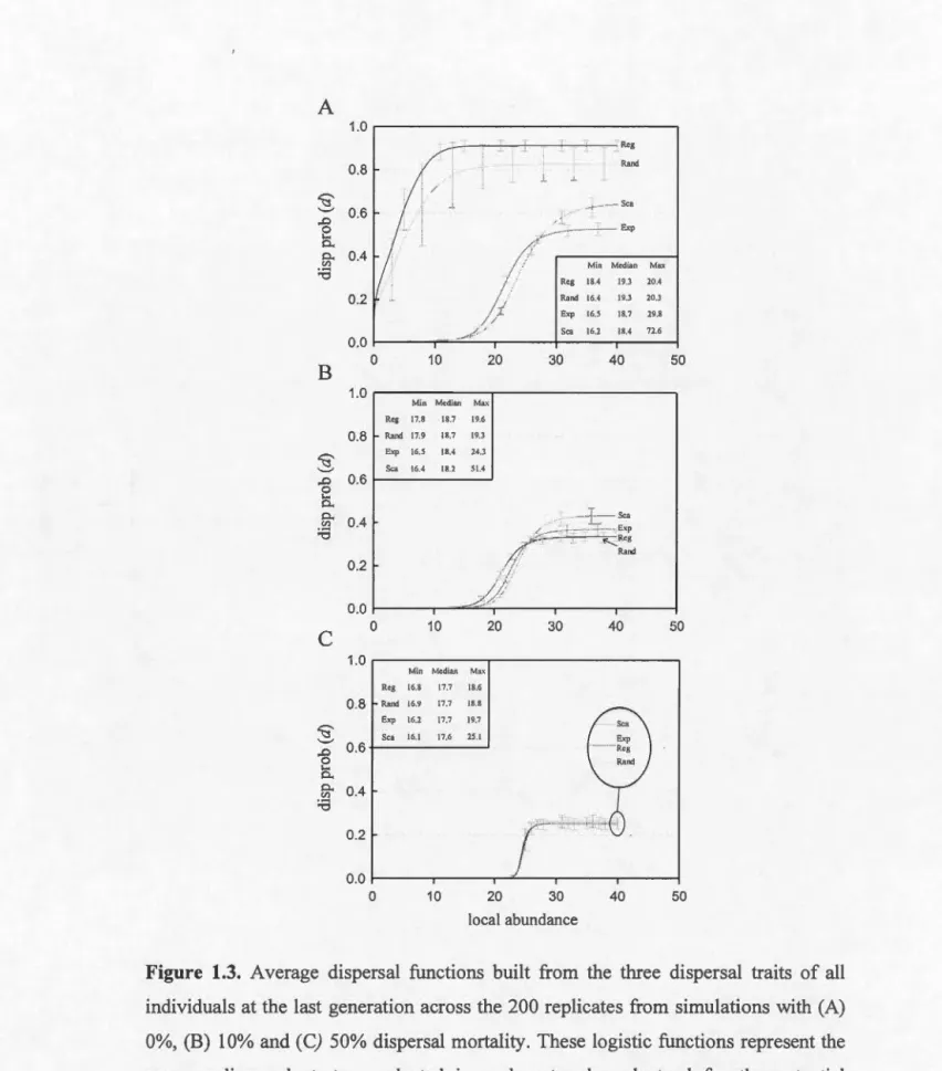
1.3
1.4
proportional to its degree. (A) Regular network, (B) random network, (C) exponential network and (D) scale-free network. Ail networks were built with 1024 patches and included 4096 connections among patches, with an average of 8 connections per patch. The networks differ in terms of their degree variance and the average degree variance across the 200 replicates for each network is: (A) 0, (B) 0.14, (C) 19.42 and (D) 48.70... ... 26 Degree distribution of (A) exponential and (B) scale-free networks. The degree distribution of exponential networks is visualized on a log-scale while the degree distribution of scale-free networks is visualized on a log-log scale... .. 28 Average dispersal functions built from the three dispersal traits of ail individuals at the last generation across the 200 replicates from simulations with (A) 0%, (B) 10% and (C) 50% dispersal mortality. These logistic functions represent the average dispersal strategy selected in each network and stand for the potential dispersal rates. Average abundances of sites on the last time step were calculated across the 200 replicates for each network in order to evaluate the realized dispersal rates. Horizontal bars represent the standard deviation of the dispersal strategies across the 200 replicates. The numbers within the squares are the minimum, median and maximum abundances across sites in each network computed on the last time step. Reg = Regular network, Rand = Random network, Exp = Exponential network and Sca = Scale-free network... 3 7 Results from two-way ANOV A Network structure (x-axis) and dispersal costs were used as fixed predictors and the average values from the 200 replicates of each dispersal trait (A) D0, (B) j3 and (C) a at the last time step as the response variable (y-axis). Each line represents a different fixed dispersal cost (c = 0.0, 0.1 or 0.5). Reg= Regular network, Rand
=
Random network, Exp=
Exponential network and Sca = Scale-free network... .... 391.6
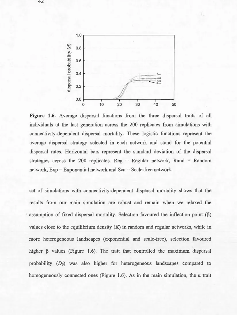
1.7
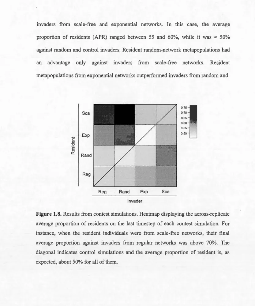
in the 10% fixed dispersal mortality scenario. In general, patches with high degree support higher local abundance and produce lower mean fitness... .. 41 Average dispersal functions from the three dispersal traits of ali individuals at the last generation across the 200 replicates from simulations with connectivity-dependent dispersal mortality. These logistic functions represent the average dispersal strategy selected in each network and stand for the potential dispersal rates. Horizontal bars represent the standard deviation of the dispersal strategies across the 200 replicates. Reg = Regular network, Rand = Random network, Exp= Exponential network and Sca = Scale-free network... .... 42 Box plots representing the distributions for the three dispersal parameters at equilibrium in the last generation. The bottom and top boundary of the box plots represent the 25% and 75% percentiles, respectively while the line within the box plots represents the median. Bottom and top whiskers outside box plots represent 10% and 90% percentiles. Data cornes from one replicate of each network type. Columns represent, from left to right, simulations with no mortality (c = 0), simulations with 10% dispersal mortality (c = 0.1) and simulations with 50% dispersal mortality (c = 0.5). (A) (D) (G) Do = maximum dispersal probability; (B) (E) (H) ~ = inflection point; (C) (F) (I) a = steepness of the curve at the inflection point. Reg = Regular network, Rand = Random network, Exp = Exponential network and Sca = Scale-free network... .... 45 1.8 Results from contest simulations. Heatmap displaying the
across-replicate average proportion of residents on the last timestep of each contest simulation. For instance, when the resident individuals were from scale-free networks, their final average proportion against invaders from regular networks was above 70%. The diagonal indicates control simulations and the average proportion of resident is, as expected, about 50% for ali of them... 46
2.2
2.3
across rows from the y-axis (C) Patches are connected to their eight nearest neighbours minus unavailable patches; for instance, the second patch is near 2 unavailable patches, thus individuals emigrating from it may only choose among the six other neighbouring patches... 63 Boxplots depicting the overall expansion speed across all scenarios for species with (A) low, (B) intermediary and (C) high growth rates. Expansion speed was measured as the identity of the outermost row (y-axis) in which the species was found at the end of the simulation. The bottom and top boundary of the box plots represent the 25% and 75% percentiles, respectively, while the line within the box plots represents the median. Top and bottom whiskers outside the box plots represent ± 1.5 times the distance between the first and third quartiles. Data beyond whiskers are outliers and plotted as dots. Significant differences between dispersal strategies within each scenario were tested using a two-sample t-test and p-values are represented as
*** P
< 0.001,*
*
p < 0.01, * p < 0.05... .... 71 Emigration rates in both density-dependent (DD) and density-independent (DI) dispersal strategies for species with low (top panel), intermediary (middle panel) and high (bottom panel) growth rates during the expansion phase. Lines in each plot represent average emigration rates, which were computed as the ratio of the number of dispersers and the pre-dispersal population size. Rates were computed across all populations (red (DD) and blue (DI) lines) or restricted to populations located in the first five rows at the expansion front (green (DD) and purple (Dl) !ines). Within each panel, top rows represent scenarios in homogeneously connected landscapes (HOM) while bottom rows represent scenarios in heterogeneously connected landscapes (HET). The left colurnn depicts scenarios with stable environment, the middle colurnn depicts scenarios with red-noise environmental fluctuation while the right colurnn depicts scenarios with white-noise environmental fluctuation... 733.2
then are allowed to expand for 2000 generation (expansion phase). The dashed square in the landscape represents a region, the scale in which diversity and GRS were measured in the analysis (see section 3.3.8). (B) Individuals survival depends firstly on how close their environmental optima phenotype (eopr) matches the local patch's environment (ex,y) and secondly (C) on the local density of conspecifics and allospecifics. Circle colours represent two different species to illustrate the three different scenarios tested for inter-specifie competition: null, half the strength of intraspecific competition or equal to intra-specific competition. (D) We tested each of these scenarios with or without mate-fin ding Allee-effects.. . . 90 General workflow for the individual-based model. The coloured squares below sexual and asexual scenarios represent the alleles of an individual for both dispersal (d) and environmental optima (eopr) phenotypes. In the sexual scenario, orange squares are male alleles whereas blue squares are female alleles and there is free recombination of alleles. In the asexual scenario there are only females and offspring inherit all alleles from the parental. In all reproductive events one offspring allele may mutate with a small probability (m). .. .. .. .. .. .. .. .. . .. .. .. .. .. .. .. .. .. .. .. .. .. .. .. .. .. .. .. .. .. .. . ... 92 3.3 Count histograms from geographie range size (GRS) distributions
across all scenarios. Species were ranked by GRS and average values were taken from the 20 replicates in each scenario. Asexual species under (A) intermediary, (B) high or (C) no competition. Sexual species under (D) intermediary, (E) high or (F) no competition... 101 3.4 Relationship between species diversity and latitude (y-axis) across all
scenarios. The red line and shaded region represent the mean and standard deviation across all replicates, respectively. Asexual species under (A) intermediary, (B) high or (C) no competition. Sexual species under (D) intermediary, (E) high or (F) no competition. Note that only 1 0 species were simulated in the scenario without interspecific competition. R2 were computed from linear regressions between diversity and latitude... 102
3.6
3.7
4.1
competition. Sexual species under (D) intermediary, (E) high or (F) no competition. Note that only 10 species were simulated in the scenario without interspecific competition. R2 were computed from linear regressions between average GRS and latitude ... . Results for range expansion speed (A, D), emigration rates (B, E) and niche evolution (C, F) for the intermediary competition scenario. Panels in the top and bottom rows refer to asexual and sexual species, respectively. Species where ranked by their abundances in all replicates and each colour represents the average values across replicates from each species. For instance, the red line in all panels represents the average value of the most abundant species across all replicates. Range expansion panels show the farthest patch in which the species was found in generation t. Emigration rates panels show the ratio between the number of dispersers and pre-dispersal population size for each species across time. Finally, niche evolution panels show the average value of the environmental optima phenotype (eopt) for each species across time ... . Results for range expansion speed (A, D), emigration rates (B, E) and niche evolution (C, F) for the scenario without interspecific competition. Panels in the top and bottom rows refer to asexual and sexual species, respectively. Species where ranked by their abundances in all replicates and each colour represents the average values across replicates from each species. Range expansion panels show the farthest patch in which the species was found in generation t. Emigration rates panels show the ratio between the number of dispersers and pre-dispersal population size for each species across time. Finally, niche evolution panels show the average value of the environmental optima phenotype (eopt) for each species across time .... Map of Canada with the 26 watersheds retained for the analysis in light orange. The dashed line represents the maximum extent of the ice caver during the last glacial maximum (LGM); modified from Blanchet et al. (2013). The arrows represent the two extreme latitudes of Canada; southem arrow: Point Peele, Ontario; northem arrow: Cape Columbia, Ellesmere Island, Nunavut ... .
104
106
107
average GRS for copepods and cladocerans. Relationship between watershed distance from the Beringian refugium and (C) its diversity or (D) average GRS for copepods and cladocerans. Red circles represent cladoceran data while green triangles represent copepod data. Each data point represents a watershed. Regression results for the se slopes are presented in Table 4.2 and Table 4.3 ... . 135
2.1 3.1 3.2 4.1 4.2 4.3
costs (c) were used as fixed predictors and the average values from the 200 replicates of each dispersal trait at the last time step as the response variable. SS
= sum of squares; MS
= mean of squares; d.f.
=
degrees of freedom, F=
F -Statistic; P=
probability. Results from both predictors and their interaction were statistically significant under an alpha-level of 0.05 ... . Simulation scenarios ... . Results from linear regressions between diversity and latitude for each scenario in which the mean and standard deviation (std) were computed across replicates. IntComp = Intermediary competition scenario; HighComp= High competition scenario.
a= intercept;
b=
regression coefficient; R2 = coefficient of determination. Results from scenarios with no competition are not shown because regressions were not significant. ... . Results from linear regressions between average GRS and latitude for each scenario in which the mean and standard deviation (std) were computed across replicates. IntComp=
Intermediary competition scenario; HighComp= High competition scenario
. a= intercept;
b = regression coefficient; R2 = coefficient of determination. Results from scenarios with no competition are not shown because regressions were not-significant. ... . Empirical evidence showing that cladocerans have better dispersal capacity than copepods ... . Mean ± standard deviation (STD), minimum (Min) and maximum (Max) values for each variable. Statistics were computed from values at the watershed level, which were computed by averaging the values across lakes within each watershed ... . Results from linear regression models between latitude and log-transformed watershed diversity (Ssm) and average geographie range size (GRS) with watershed area (A) as a covariable. Global - P = global probability; PINTER = probability for the intercept; PLAT = probability for latitude; PA = probability for watershed area; bLAT = coefficient for latitude; bA= coefficient for watershed area. Significant p-values under an a = 0.05 are highlighted in bold ... .38 69 103 105 124 129 136
4.5
probability for the intercept; PsER = probability for distance from the Beringian refugium; bsER =coefficient for distance from the Beringian refugium; PA = probability for watershed area; bA = coefficient for watershed area. Significant p-values under an a= 0.05 are highlighted in bold. *Given that the residuals from this model were not homoscedastic, we applied the Hu ber-White method, which gives heteroscedastic corrected estima tes for the linear model. ... .
Result from forward-selection regressiOn models between
environmental variables and diversity and average geographie range size (GRS) of watersheds for both cladocerans and copepods. VARJ and VAR2 refer to the variables selected in the forward-selection procedure. MeanA T = Mean Annual Temperature; MDGSR = Mean Daily Global Sol ar Radiation; T AP = Total Annual Precipitation;
MDBS = Mean Duration of Bright Sunshine; M_ELE = Mean
Elevation; bvARI = regression slope for the first selected variable, bvAR2 = regression slope for the second selected variable; PvARI = probability for the first selected variable; PvAR2 = probability for the second selected variable; bA = coefficient for watershed are a; PA = probability for watershed area. Significant p-values under an a=0.05 are highlighted in bold ... .
137
ces aires de distribution et un nombre important d'études théoriques et empiriques s'est concentré à identifier les éléments affectant 1 'évolution des traits de dispersion. Cependant, il y a encore des lacunes dans nos connaissances concernant l'influence de processus tels que les interactions biotiques, la connectivité du paysage, l'adaptation locale et l'effet Allee sur l'évolution de la dispersion et des dynamiques des distributions des espèces. En générale, pour qu'une espèce étende son aire de répartition, les individus doivent être capables de se disperser dans une nouvelle région et ensuite de tolérer les nouvelles conditions abiotiques et biotiques rencontrées. Finalement, ils doivent pouvoir se reproduire pour soutenir une population viable. Alors que les approches statistiques (i.e., corrélatives) sont suffisantes pour évaluer l'importance des facteurs climatiques sur la distribution géographique d'une espèce (i.e., tolérance environnementale), elles sont moins efficaces pour les autres processus mentionnés ci-dessus. Par ailleurs, les échelles spatiales et temporelles sur lesquelles ces facteurs agissent font en sorte que l'utilisation d'approches expérimentales pour évaluer leurs effets est peu éthique, voir impossible. Conséquemment, je propose l'utilisation de modèles centrés sur l'individu (MCI) encadrés dans la théorie des métapopulations pour évaluer l'importance relative des processus influençant l'évolution de la dispersion et l'expansion des aires de répartition des espèces. Finalement, à travers l'étude de ces dynamiques, mon but est d'explorer les mécanismes structurant les patrons de biodiversité à large échelle. Les MCis, par définition, prennent en compte la variation intraspécifique des traits et, de plus, ils tiennent compte des interactions adaptatives entre les individus et avec leur environnement. À ce titre, les MCis fournissent l'agencement idéal pour évaluer comment les dynamiques écologiques et évolutives se déroulant aux petites échelles peuvent structurer des patrons écologiques aux larges échelles spatiales. Cette thèse est composée de trois chapitres utilisant les MCis et un quatrième basé sur une base de données de zooplancton d'eau douce, qui sera utilisée pour tester quelques prédictions obtenues des MCis. Le Chapitre I explore l'effet de la variation dans les degrés de connectivité des parcelles d'habitat dans des paysages sur l'évolution des stratégies de dispersion. Le Chapitre II vise à déterminer l'effet des facteurs abiotiques (niveau de connectivité et de fluctuations environnementales) sur la vitesse d'expansion d'une espèce à travers un paysage hétérogène. Plus précisément, j'évalue quelle des stratégies de dispersion denso-dépendante ou denso-indenso-dépendante induit des taux d'expansion plus rapides pour des espèces asexuées qui varient dans leur taux de croissance. Dans le Chapitre III, je développe un modèle multi-espèces pour comprendre comment les processus biotiques tels que l'effet Allee et la compétition interspécifique peuvent influencer l'expansion des aires de répartition des espèces à travers un paysage hétérogène.
de 1600 lacs au Canada. À cause de leurs modes de reproduction contrastés (cyclique parthénogénétique pour les cladocères et sexué pour les copépodes), ces deux clades diffèrent par rapport à leur susceptibilité à l'effet Allee et à leurs capacités de dispersion et d'adaptation locale.
Les résultats obtenus des MCis fournissent des évidences par rapport à la façon dont les facteurs abiotiques et biotiques modulent 1' évolution de la dispersion laquelle, à son tour, influence la taille des aires de répartition des espèces et les patrons de diversité à travers de larges échelles spatiales. Le Chapitre I démontre que différentes stratégies de dispersion peuvent évoluer en réponse à la structure spatiale du paysage. Le Chapitre II montre que la dispersion dense-dépendante permet une expansion plus rapide à travers un gradient environnemental seulement quand le taux de croissance des populations est élevé. Le Chapitre III illustre que 1' effet Allee et la force de la compétition interspécifique peuvent moduler les gradients latitudinaux de diversité et d'aires de répartition. Finalement, le Chapitre IV démontre que les cladocères, des organismes ayant surtout une reproduction parthénogénétique et qui ne sont pas susceptibles à l'effet Allee, présentent, en moyenne, des aires de répartition significativement plus larges que les copépodes ayant une reproduction sexuée. Par ailleurs, les deux clades diffèrent énormément par rapport à leurs gradients latitudinaux de diversité et de répartition : le nombre d'espèces de cladocères décroît et leur aire de répartition moyenne s'accroît de manière importante vers les latitudes nordiques tandis que les copépodes ne présentent aucun patron latitudinal vis-à-vis de ces deux caractéristiques. Ainsi, cette thèse démontre que l'évolution de la dispersion et 1' adaptation locale sont des facteurs clés pour comprendre la dynamique des aires de répartition (i.e., contraction et expansion) et que les processus qui se produisent aux petites échelles, tels que l'effet Allee et les interactions biotiques, peuvent influencer des patrons observables aux larges échelles spatiales comme la taille des aires de répartition des espèces et les gradients macroécologiques.
Mots-clés: Dynamiques des aires de répartition, zooplancton, gradient latitudinal de diversité, dispersion contexte-dépendante, structure du paysage, chevauchement de 1 'utilisation des ressources, loi de Rapoport
focusing on the drivers of dispersal evolution. However, there are still sorne knowledge gaps regarding the interaction between dispersal evolution and other processes such as biotic interactions, landscape connectivity, local adaptation and Allee-effects in regulating range dynamics. For a species to spread its range, individuals first need to be capable of dispersing into a novel region, then tolerate the local abiotic and biotic environment and finally they should be able to reproduce in arder to sustain a viable population. While statistical (i.e., correlative) approaches are enough to assess the importance of the environment on species geographie distributions (i.e., environmental tolerance), the same is not true for the above-mentioned processes. Furthermore, the spatial and temporal scales in which the proce~ses regulating species ranges act make it unethical or impossible to evaluate them through experimental approaches. Therefore, I propose to use individual-based models (IBM) under a metapopulation framework in arder to evaluate the relative importance of these drivers on dispersal evolution and range expansion. Ultimately, through the lenses of species range dynarnics, I aim at exploring the mechanisms underlying large-scale biodiversity patterns. IBMs by definition account for intraspecific variation in traits and, more important! y, allow individuals to have adaptive interactions with each other and their environment. As such, IBMs provide the fundamental layout to evaluate how eco-evolutionary dynamics at small scales shape ecological patterns at larger scales. This thesis is comprised of three chapters using IBMs and a fourth that is based on a large-scale empirical dataset of freshwater zooplankton, which is used to test sorne predictions obtained from the models. Chapter I explores how landscapes with different degrees of connectivity among their habitat patches may affect the dispersal evolution. Chapter II investigates how abiotic factors influence the speed of range expansion across a heterogeneous landscape. Specifically I ask whether density-dependent (DD) or density-independent (DI) dispersal strategies induce faster range expansion rates to asexual species with varying growth rates in landscapes with different degrees of patch connectivity and levels of environment fluctuation. In Chapter III, I implementa multi-species madel to understand how biotic processes such as Allee effects and interspecific competition may affect the range expansion of species across a heterogeneous landscape and, ultimately, how diversity gradients are structured by these interactions. Lastly, in Chapter IV, I evaluate how geographie range size (GRS) and latitudinal gradients in diversity and range-size differ between copepods and cladocerans using a large-scale dataset of freshwater microcrustacean species distributed across + 1600 lakes in Canada. Given the ir contrasting ma ting system ( cyclic parthenogenetic cladocerans and obligate sexual copepods), these two clades differ in their susceptibility to Allee effects, dispersal ability and capacity of adaptation.
expansion across an environmental gradient when population growth is high. Chapter III shows that both Allee-effects and the strength of interspecific competition modulate the steepness of latitudinal gradients in diversity and GRS. Finally, chapter IV shows that cladocerans, parthenogenetic species which do not suffer from mate-finding Allee effects, have a much larger ranges than sexual copepods. Both clades also have contrasting patterns regarding latitudinal gradients, in which the number of cladoceran species decrease and average GRS increase towards northern latitudes while copepods do not show any latitudinal pattern in either of these properties. Thus this thesis shows that dispersal evolution and local adaptation are of central importance to understand range dynamics (i.e., expansion and contraction) and that processes occurring at local scales such as Allee effects and biotic interactions may scale up to influence both species GRS and the structure of macroecological patterns. Keywords: Range dynamics, zooplankton, latitudinal-diversity gradient, context-dependent dispersal, landscape structure, resource-use overlap, Rapoport's rule
species not able to adapt to every type of environment? Why do sorne species attain broad distributions whereas most do not? Can we understand biodiversity patterns through the mechanisms affecting species geographie range sizes? These are, among others, central questions in macroecology. Answering them will help understanding the patterns of diversity that are observed across Earth. In the present work, I will tackle a series of processes that contribute to species range dynamics. Among these processes, dispersal is a key component. Dispersal allows species to fmd new suitable habitats and affects the dynamics of adaptation to novel environmental conditions that they might encounter while expanding their geographie ranges. Moreover, dispersal is an evolvable trait influenced by the relative importance of factors that either improve fitness of dispersing individuals or increase the cost of dispersal. However, there are still many gaps in our understanding of how dispersal interacts with other processes such as Allee effects (i.e., decreased average individual fitness at low population density), landscape spatial structure and biotic factors and how these interactions shape macroecological patterns such as latitudinal diversity gradients and Rapoport's rule. Through a combination of computer simulations and analyses of empirical data from zooplankton communities, 1 explore sorne of these questions in a multi-scale framework, ranging from individual decisions up to large-scale distributional patterns.
Below, I give a brief overview on ecological and evolutionary processes driven by species dispersal at multiple ecological scales, their implication for species geographie ranges, and how they might influence the distribution of freshwater zooplankton. I then explain how the use of individual-based models can help to tackle sorne of these questions. Finally, I outline the main goals of the chapters from this thesis.
0.1 Multi-scale eco-evolutionary dispersal processes and their consequence for range dynamics
Dispersal is one of the most studied concepts in evolutionary ecolo gy, especially given its various implications in ecological dynamics and longstanding impacts in evolutionary processes (reviewed in Bowler & Benton, 2005; Ronce, 2007; Travis et al., 2013; Kubisch et al., 2014). It is now widely accepted that dispersal is at the core of species geographie range formation (Sexton et al., 2009). Most if not all species are capable of dispersing during sorne life stage and at a particular spatial scale, which allows them to persist in an ever changing environment (Ronce, 2007). Here I define dispersal as an active or passive attempt to move away from a natallbreeding population to establish into another breeding population, with potential effects for gene flow (Clobert et al., 2009; Travis et al., 2012). This process can be divided into three distinct stages: departure, transience and settlement (Bonte et al., 20 12; Travis et al., 2012). As individuals tend to disperse to habitats around their natal population,
spec1es are non-randomly distributed across space, generally forming cohesive geographie ranges (Rahbek et al., 2007). The limits of species' geographie ranges are a result of the interplay between ecological and evolutionary process (Holt, 2003;
Kubisch, 20 12) that operate at a broad range of spatial and temporal scales, from
small-scale decisions made at the individual leve! up to global climate drivers and
major biogeographie events.
0.1.1 Dispersal evolutionary dynamics
In arder to properly understand range dynamics, it is important to know how the
different selective agents affect an individual's decision to disperse. Generally,
individuals disperse in arder to match their phenotype against prevailing
environmental conditions as a way to improve their fitness (Ronce, 2007). However,
dispersal is a risky behaviour, involving cost during bath transfer (e.g., predation risk,
failing to find suitable habitats) and settlement phases (e.g., lower competitve ability
or fecundity compared to residents; Bonte et al., 20 12). Therefore, individuals may decide not to disperse if the risk of leaving a patch outweighs any fitness gains they
might attain in another patch (Bowler & Benton, 2005). These findings, together with the fact that dispersal traits are heritable (Saastamoinen, 2008), imply that dispersal is
subject to evolution (Bowler & Benton, 2005; Ronce, 2007). In addition, except for passive dispersal, dispersal decisions are generally non-random and rely on
Species may disperse based on an assessment of local population density, a strategy named density-dependent dispersal (Poethke & Hovestadt, 2002; Travis et al., 2009). On one hand, individuals will be more likely to leave crowded patches in order to avoid high competition for local resources (Hamilton & May, 1977; French & Travis, 2001; Bitume et al., 20 13). On the other hand, Allee effects (i.e., a decrease in average individual fitness when population density is low; Courchamp et al., 1999) may reverse this tendency. For example, finding suitable mates for sexually reproducing species is a limiting factor; therefore leaving high-density patches may decrease an in di vi dual' s chance of reproduction. Another process that affects dispersal evolution is environmental fluctuation; species dwelling in a habitat with large fluctuations (i.e., high variance) tend to have high dispersal rates in order to cope with temporal variability in resource availability (McPeek & Holt, 1992; Travis & Dytham, 1999) or simply to avoid local extinction (Poethke et al., 2003). By spreading out offspring in a landscape in which conditions are highly stochastic, long-term average fitness is increased by lowering the temporal variance in fitness, a phenomenon named "bet-hedging strategy" (Philipi & Seger, 1989). Furthermore, high dispersal rates may be favoured due to spatial selection,
a
phenomenon that has been extensively studied in invasive species (Duckworth, 2008; Phillips et al., 201 Oa). Spatial selection happens during range expansion, in which the most dispersive individuals are generally the ones found at the range border. Therefore, it is likely that they will mate with each other and thus produce highly dispersive offspring (Phillips et al., 201 Ob). These individuals have higher fitness compared toindividuals from core populations due to the low competitive environment found at
the expansion front, which results in an increased frequency in dispersive phenotypes
(Brown et al., 2013). Together, these processes promote a dramatic increase in the
overall dispersal rate of the species. For instance, a study reported a five-fold increase in cane toads dispersal rates since the invasion began in Australia due to spatial selection (Phillips et al., 201 Ob).
Ultimately, almost all species upon close inspection exhibit sorne degree of internai
spatial structure, even in seemingly continuous habitat. Consequently, understanding
the processes driving dispersal evolution can be undertaken in a metapopulation framework (i.e., spatially distinct populations linked by dispersal; Hanski & Beverton, 1994; Hanski, 1998). Whether an individual disperses or not between populations is contingent on the spatial structure of habitat patches, which regulates
the flow of individuals ac ross any given landscape (Baguette et al., 2013; Grilli et al.,
2015). Therefore, landscape connectivity may have potential demographie consequences to local populations if it promotes asymmetric dispersal among them. If
species are using a density-dependent dispersal strategy, landscape connectivity may
indirectly influence dispersal evolution through its effects on population's
0.1.2 Dispersal and metapopulation dynamics
Metapopulation population theory arms at understanding the colonization and
extinctions dynamics of patchy populations (Hanski, 1998; Fortuna et al., 2006). Species may persist regionally even if they go extinct in a local patch, which may be
later recolonized by immigration from neighbouring populations. The species
geographie range s1ze is essentially the result of these dynamics, expanding or
contracting depending on the relative importance of extinction and colonization (Kubisch et al., 20 16). Furthermore, dispersal among populations have important consequences for processes of local adaptation (Lenormand, 2002). Dispersal may
allow populations to persist in unfavourable environments (i.e., negative net
population growth) through source sink-dynamics (Pulliam, 1988). Depending on the
harshness of the sink's environment, immigration may promote adaptation by
increasing population size and genetic diversity, two pre-requisites for evolution by
natural selection (Lenormand, 2002), thus allowing species to expand their ranges
into previously unsuitable habitats (Holt & Barfield, 2011). However, dispersal may
hinder local adaptation if mating between resident and immigrants imposes a reproductive cost and reduces the average individual fitness in the sink population, a
process named migration load (Lenormand, 2002). Migration load can slow or
prevent range expansion when an asymmetric flow of individuals from core to
peripheral populations precludes these populations to adapt to novel environmental
promote or prevent local adaptation is contingent on its intensity and the steepness of the environmental gradient.
0.1.3 Metacommunity dynamics, biotic interactions and their consequences for species geographie ranges
It is reasonable to assume that no single species lives alone in nature, therefore we use the metacommunity concept as the basic framework to understand how range dynamics may be affected by other species (Case et al., 2005). Metacommunity theory is an extension of the metapopulation theory that aims at understanding the relative importance of abiotic factors, interspecific interactions and dispersal processes to both local community and regional pool assembly (Wilson, 1992;
Leibold et al., 2004; Henriques-Silva et al., 2013; Fernandes et al., 2014). For instance, metacommunity theory shows that species can co-exist regionally through dispersal even if a superior competitor drives an inferior competitor to extinction in a local community (Mouquet & Loreau, 2002). These effects compound over multiple species and determine the local and regional ric~ess of a particular habitat patch or regwn, respectively. Similarly to metapopulations, dispersal effects on metacommunity dynamics are contingent on its intensity. For instance, the above-mentioned co-existence process is only possible at intermediary levels of dispersal. An inferior competitor may be driven to regional extinction if the su peri or competitor sustains high dispersal rates (Mouquet & Loreau, 2002). If competitive abilities are
similar, then community assembly may be contingent on priority effects in which the
first species to colonize a new patch has an advantage over species colonizing later
(Fukami, 20 15). For instance, earl y colonizers may reduce the availability of local
resources ( e.g., light, space, nutrients) for later-arriving species, a pro cess named
niche pre-emption (Fukami, 20 15). Finally, evolutionary dynamics may enhance
priority effects if local adaptation of early colonizers improves their ability to
monopolize local resources (Loeuille & Leibold, 2008; Urban et al., 2008; Urban & De Meester, 2009; Vanoverbeke et al., in press).
0.1.4 Range dynamics and large-scale diversity patterns
The identity and number of spec1es distributed across the globe vary and
understanding what drives these patterns has been a long-standing goal in
macroecology and biogeography (Willig et al., 2003). However, the ecological and evolutionary processes regulating these patterns operate at spatial and temporal scales
in which experimental or manipulative studies are logistically unethical or
impossible. As Hay don et al. ( 1993: p.ll7) stated: "The pro cess of replication and repeatability, usually fundamental to the testing of scientific hypothesis, are not
available for biogeographers". Thus, correlative approaches (i.e., curve-fitting
models) have dominated this field over the last decades ( e.g., Currie, 1991; Hawkins
Unfortunately, so far there are no satisfactory explanations for the relative importance
of mechanisms underlying diversity gradients given that multiple factors may show
correlation, without necessarily having a causal link, with richness (Currie et al.,
1999; Peres-Neto & Legendre, 2010). As a consequence, there has been a recent shift
to tackle this problem through more mechanistic models (e.g., Rahbek et al., 2007;
Range! et al., 2007; Gotelli et al., 2009; Buschke et al., 20 15), consisting of a bottom-up approach were one explicitly simulates the mechanisms thought to underlie range
dynamics and then evaluate if the outcomes of the model predict a pattern or fit
empirical data (Grimm & Railsback, 2005; Gotelli et al., 2009; Cuddington et al.,
2013). In these models, species will probabilistically spread across a landscape based
on certain characteristics of available cells ( e.g., their environment, proxirnity to cells
occupied by the focal species). This process can be repeated for multiple species,
where estimates of species diversity are computed based on the overlap of species
ranges within each geographie cell (Rahbek et al., 2007; Buschke et al., 20 15). In this
case, the interactions of processes regulating multi-species range expansion will
promote patterns of diversity across geographical cells according to their properties
(e.g., their abiotic conditions, spatial isolation) (Gotelli et al., 2009). Nevertheless,
mechanistic models rely heavily on imposed responses in which desired outcomes are
forced into the model. For instance, rriechanistic-models generally constrain the range
size of simulated species to follow a similar distribution of empirical range values
(e.g., Buschke et al., 2015). Further, mechanistic models assume that species are
a limited capacity to account for eco-evolutionary dynamics because spectes lack intraspecific variation and adaptive responses. Trait variation has been recognized to be fundamental in classical work of niche evolution (Roughgarden, 1972; Grant & Grant, 2002), which is one way that species can expand their ranges (Davis & Shaw, 2001 ). Ecological processes are also affected by intraspecific variation. For instance, variation in phenotype-local environment matching may prevent species range from contracting in highly fluctuating environments by promoting persistence through portfolio effect (Bolnick et al., 2011 ). Dispersal traits also show great variation among conspecifics (Stevens et al., 201 0), especially between core and marginal populations (Kubisch et al., 2011) which may influence the speed of range expansion (Phillips et al., 201 Oa). Neglecting intraspecific variation may th us hinder our ability
to understand the multiple processes underlying species range dynamics (Stevens et al., 2010; Bolnick et al., 2011) and other large-scale ecological patterns (Araujo & Costa-Pereira, 2013).
0.2 Individual-based models in macroecology
Individual-based models (IBM) allow relaxing the above-mentioned assumptions. First, IBMs rely less on imposed responses because they allow complex interactions between their lower-level components and the consequent emergence of system-level properties from these interactions (Grimm & Railsback, 2005). Second, lower-level components in IBMs are, as suggested by their name, unique individuals with
characteristics that set them apart from every other individual. As a consequence,
IBMs incorporate intraspecific variation by default. Finally, IBMs allow for individuals to exhibit adaptive response among them and between them and their environment. This approach stems from a general framework used in science known as "Complex Adaptive Systems" (CAS) which attempts to generate knowledge of a
given system based on its interacting, adaptive agents (Levin, 1998; Railsback, 2001). Bath intraspecific variation and the adaptive nature of lower-level components within
IBMs provide the fundamental layout for an evolutionary perspective to be included in the madel, that is, one that recognizes and explores the properties of ecological
entities as a CAS whose components are subject to natural selection (Levin, 1998).
This property is essential for understanding relationships and feedbacks between
ecological and evolutionary processes (i.e., eco-evolutionary dynamics), especially given that it is increasingly recognized that evolution can occur on ecological timescales (Schoener, 2011 ). Therefore, spatially explicit IBMs are a useful tool to ask questions about macroecology patterns as they may incorporate dispersal, local
adaptation, Allee effects, biotic interactions and many other processes involved in range dynamics (Travis & Dytham, 1998; Burton et al., 2010; Kubisch et al., 2013b;
0.3 Study system
In the present work I propose to apply IBMs in a multi-scale framework to ask questions ranging from dispersal evolution, to abiotic and biotic factors influencing range dynamics and diversity patterns. Finally, 1 evaluate sorne of the predictions obtained from the IBMs on large-scale patterns in freshwater microcrustacean zooplankton. This taxonomie group is an interesting study system because it is composed of species that differ widely in breeding modes (Allan, 1976; De Meester, 1996), which have many implications for dispersal and local adaptation processes.
Cladocerans almost invariably reproduce through cyclic parthenogenesis, that is, several rounds of cloning interrupted by occasional sexual reproduction. Generally, females emerge at the beginning of the growing season and reproduce through amictic parthenogenesis (i.e., without fertilization) as long as environmental conditions are favourable (De Meester, 1996). When an environment starts to deteriorate, either by depletion of resources, overcrowding or the onset of unsuitable conditions (e.g., winter, drought), females produce males through parthenogenesis and haploid eggs, which are fertilized by males (De Meester, 1996). These sexual eggs represent the diapausing phase of cladocerans and will hatch as soon as favourable conditions are restored. In addition, sorne cladoceran species also have completely asexual populations, either through obligate apomictic parthenogenesis (Dufresne & Hebert, 1997) or self-fertilization (Hebert et al., 2007) where
female-only populations are able to produce diapausing eggs. The capacity to reproduce
asexually is a great advantage to cladocerans, as it improves their dispersal ability by
allowing them to establish new populations with solely one individual (Havel & Shurin, 2004; Gray & Arnott, 2011).
The copepod mating system differs from cladocerans in its obligate sexuality.
Fertilized eggs hatch into a larval phased called the nauplius. Subsequent larval and
juvenile (i.e., copepodid) stages occur before reaching the adult phase, when
individuals attain sexually maturity (Allan, 1976). During the mating phase, females
may store sperm in a spermathecal sac, lessening the need for further breeding. The
diapausing phase differ in the two main groups of copepods: calanoid copepods
undergo diapause during the egg stage whereas the cyclopoid copepods encyst and
diapause during juvenile stages, generally as C3-C4 copepodites (Fryer, 1996; Frisch,
2002). Given their life-cycle, copepods suffer from Allee effects when colonizing a
new water body and experimental evidence has shown that cladocerans are better
colonizers than copepods, as the latter are limited by mate-finding difficulties at low
densities (Kramer et al., 2008; Gray & Arnott, 2011; Frisch et al., 2012).
Despite the island-like nature of lakes and ponds, which implies that they are
generally isolated from one another by an inhospitable terrestrial matrix, freshwater
microcrustaceans have shown incredible success at dispersing (Havel & Shurin, 2004; Frisch et al., 2012). Dispersal occurs generally during the diapausing stage,
when the orgamsms may resist freezing, desiccation and even digestion, thus remaining viable through the harsh conditions of overland dispersal (Havel & Shurin, 2004). Cladocerans diapausing eggs are often enveloped by ephippial capsules that have spines, barbs or air-trapping dimples that improve buoyancy, which increase their capacity of hitchhiking via dispersal vectors (Fryer, 1996). With the exception of occasional free-swimming adult emigration through watercourses, dispersal mainly occurs passively, either via wind (Caceres & Soluk, 2002; Horvath et al., in press), human assistance (e.g., recreational boats, ship ballast tanks; Havel & Shurin, 2004) or animal vectors such as marnmals and waterbirds (Figuerola et al., 2005). Particularly, waterfowls are important animal vectors for long distance dispersal of zooplankton. For instance, studies have shown that the population genetic structure of sorne microcrustacean species is related to the north-south migration routes of these animais (Taylor et al., 1998; Figuerola et al., 2005).
Substantial ecological and evolutionary research has been done on zooplankton, especially at small scales. Zooplankton are used to understand how different processes such as local-adaptation (Van Doorslaer et al., 2009; De Meester et al., 2011), dispersal (Vogt & Beisner, 2011), biotic interactions (Lynch, 1979), Allee effects (Gray & Arnott, 2011) and priority effects (De Meester et al., 2002; Louette & De Meester, 2007) affect comrnunity assembly. Larger scales studies have also been undertaken to disentangle the relative importance of local and regional processes underpinning the structure of multiple zooplankton communities (e.g., Pinel-Alloul,
1995; Pinel-Alloul et al., 1995; Cottenie et al., 2003; Beisner et al., 2006). At
continental and global scales, however, studies are scarce and show different results.
For instance, Pinel-Alloul et al. (2013) and Hessen et al. (2007) showed that
freshwater microcrustacean diversity is tightly related to energy-related variables
whereas Mazaris et al. (20 1 0) found only a weak relationship with environmental
drivers. However, ali these studies pooled both cladocerans and copepods in the sarne
analysis. It is expected that they respond to different drivers due to their different
mating system (Leibold et al., 201 0), which are known to have potential
consequences for their susceptibility to Allee effects, dispersal capacity, and local
adaptation processes (Hargreaves et al., 2014; Grossenbacher et al., 2015). As
discussed previously, ail these processes affect species range dynarnics, thus we may
expect that these two groups of species will differ in their geographie range size as well.
0.4 Thesis outline
The goal of this thesis was to explore the various factors affecting species range dynarnics with IBMs and test sorne of these predictions on a large-scale dataset of
freshwater microcrustaceans. To this end, the present work is comprised of four
chapters, three using individual-based models and one with empirical data:
Chapter II - Range expansion depends on the interaction between dispersal strategies and population growth rate
Chapter III - Biotic processes during range expansion explain large-scale diversity gradients
Chapter IV - Mating system, climate and history interact in explaining macroecological patterns in freshwater zooplankton
In Chapter I the effect of variance in connectivity among patches on the evolution of density-dependent dispersal strategies was explored. I simulated landscapes that varied in their connectivity structure using network models. Landscapes ranged from ali patches having the same number of connections to landscapes with high variability in connectivity (i.e., a few patches with many connections and many patches with a few connections). Landscapes were seeded with individuals exhibiting many different dispersal strategies and we evaluated which ones were selected across the different landscape configurations:
The goal of Chapter II was to investigate how abiotic factors such as landscape connectivity and environmental fluctuation would affect the spread rate of species with different dispersal strategies acros.s an environmental gradient. We contrasted the range expansion speed of species with different levels of growth rates following either density-dependent or density-independent dispersal in landscapes with contrasting connectivity structures and degrees of environmental fluctuation.
Chapter III explored how biotic factors such as Allee effects and interspecific competition would influence the range expansion of multiple species on a heterogeneous landscape. Further, 1 was interested in evaluating how these effects on species range dynamics would influence emergent patterns of biodiversity across the landscape (i.e., latitudinal diversity gradient and Rapoport's rule). 1 simulated an out-of-the tropics mode!, in which 1 assumed that species originated in the tropics and expanded their ranges towards northern latitudes. Species were initially equivalent in respect to their dispersal capacity and environmental niche, but these traits were allowed to evolve during the simulation. 1 varied the degree of interspecific competition among species and 1 tested for Allee effects by contrasting two mating systems: asexual and sexual, in which the latter is subject to mate-finding difficulties at low densities. Ultimately, we measured the final range size of all species at the end of the simulation in each replicate and evaluated the steepness of diversity and range-size gradients across the landscape.
Chapter IV was conducted to test sorne of the predictions derived from the IBM in Chapter III on a large-scale dataset of freshwater zooplankton distribution in Canada. 1 first evaluated the geographie range size distribution of cladocerans and copepods.
Given that they differ in their susceptibility to mate-finding Allee effects due to their different mating-systems, their range-size distributions should be similar to the ones predicted for the sexual and asexual species in the previous chapter for the asexual
and sexual spec1es. Second, I analyzed the steepness of latitudinal gradients of
diversity and geographie range size (i.e., Rapoport's rule) for each group. Given that
their contrasting life-history traits may affect how they respond to environmental
drivers and historical factors (i.e., dispersal limitation), it should translate into
contrasting latitudinal-diversity gradients and Rapoport's rule.
To sumrnanze, results obtained from the IBMs along chapters I to III provide
evidence regarding how abiotic and biotic factors modulate the evolutionary
dynamics of dispersal, which in turn shape species geographie ranges. Further, the
multi-species model in chapter III uncovers previously overlooked factors regulating
diversity patterns at large spatial scales. Chapter IV shows that sorne of these
mechanisms, such as mate-finding Allee-effects, may have deep impacts on
R. Henriques-Silva, F. Boivin, V. Calcagno, M. C. Urban and P. R. Peres-Neto Published: Proceedings of the Royal Society B: Biological Sciences (2015) 282: 20142879
DOl: 10.1 098/rspb.20 14.2879
1.1 Summary
Dispersal has long been recognized as a mechanism that shapes many observed ecological and evolutionary processes. Thus, understanding the factors that promote its evolution remains a major goal in evolutionary ecology. Landscape connectivity may mediate the trade-off between the forces in favour of dispersal propensity (e.g., kin-competition, local extinction probability) and those against it ( e.g., energetic or survival costs of dispersal). It remains, however, an open question how differing degrees of landscape connectivity may select for different dispersal strategies. We implemented an individual-based model to study the evolution of dispersal on landscapes that differed in the variance of connectivity across patches ranging from networks with all patches equally connected to highly heterogeneous networks. The parthenogenetic individuals dispersed based on a flexible logistic function of local
abundance. Our results suggest, all else being equal, that landscapes differing in their
connectivity patterns will select for different dispersal strategies, and that these
strategies confer a long-term fitness advantage to individuals at the regional scale. The strength of the selection will, however, vary across network types, being stronger on heterogeneous landscapes compared to the ones where all patches have equal connectivity. Our findings highlight how landscape connectivity can determine the
evolution of dispersal strategies, which in turn affects how we think about important
ecological dynamics such as metapopulation persistence and range expansion.
1.2 Introduction
Dispersal is a key factor in both ecology and evolution (Ronce, 2007). From an ecological perspective, dispersal may affect population and community dynamics
(Hanski, 1994; Mouquet & Loreau, 2002), rescue populations from extinction (Brown & Kodric-Brown, 1977), shape species distributions (Olden et al., 2001), and
allow species to track favourable environmental conditions and influence the rate at which species expand the ir ranges (Travis et al., 2009). From an evolutionary
perspective, dispersal can produce gene flow and depending on its magnitude, can
preclude or promote local adaptation and speciation, increase or decrease local
genetic diversity, mitigate the effects of drift in small populations and reduce mutation load (Roff & Fairbairn, 2001; Alleaume-Benharira et al., 2006; Ronce, 2007). As such, natural selection is expected to act on traits associated with dispersal