Etude des propriétés thermodynamiques des nouveaux fluides frigorigènes

(1)

HAL Id: tel-01804996

https://pastel.archives-ouvertes.fr/tel-01804996

Submitted on 1 Jun 2018

HAL is a multi-disciplinary open access

archive for the deposit and dissemination of sci-entific research documents, whether they are pub-lished or not. The documents may come from teaching and research institutions in France or abroad, or from public or private research centers.

L’archive ouverte pluridisciplinaire HAL, est destinée au dépôt et à la diffusion de documents scientifiques de niveau recherche, publiés ou non, émanant des établissements d’enseignement et de recherche français ou étrangers, des laboratoires publics ou privés.

fluides frigorigènes

Jamal El Abbadi

To cite this version:

Jamal El Abbadi. Etude des propriétés thermodynamiques des nouveaux fluides frigorigènes. Génie chimique. Université Paris sciences et lettres, 2016. Français. �NNT : 2016PSLEM089�. �tel-01804996�

(2)

Soutenue par Jamal

EL ABBADI

le 02 Décembre 2016

h

THÈSE DE DOCTORAT

de l’Université de recherche Paris Sciences et Lettres

PSL Research University

Préparée à MINES ParisTech

Dirigée par :

Christophe COQUELET

Céline HOURIEZ

h

Etude des propriétés thermodynamiques des nouveaux fluides

frigorigènes

Thermodynamic properties of new refrigerants

COMPOSITION DU JURY :

M. Pascal TOBALY

CNAM, Président

M. J.P. Martin TRUSLER

Imperial College London, Rapporteur

M. Romain PRIVAT

ENSIC - LRGP, Rapporteur

M. Bernard ROUSSEAU

Université Paris-Sud, Examinateur

M. Patrice PARICAUD

ENSTA ParisTech – Université Paris Saclay, Examinateur

M. Christophe COQUELET

Mines ParisTech – PSL Research University, Examinateur

Mme. Céline HOURIEZ

Mines ParisTech – PSL Research University, Examinateur

Ecole doctorale

n°432

Sciences des Métiers de l’Ingénieur

(3)

(4)

i

To Mom and Dad

To my sisters Nadia and Ibtissam

(5)

ii

Acknowledgments

First, I would like to thank my Directeur de thèse Prof. Christophe Coquelet for according me this wonderful opportunity to do my PhD at the CTP, for his great supervision and guidance, for his great help and support all along my thesis, for the great discussions we had, and for constantly pushing me to reach my full potential and be a better scientist.

I would also like to thank my Maître de thèse Dr. Céline Houriez, for her great supervision and guidance, for her continuous support and help, for her precious advices and the great discussions we had, for always checking on me, and for continuously believing in me.

Then, I would like to thank Prof. J.P. Martin Trusler for welcoming me into his research group at Imperial College London, for his tremendous help and support, for his precious advices and guidance, for helping me with the experimental work, and for his hospitality.

I would like to thank the members of the jury: Prof. J.P. Martin Trusler and Dr. Romain Privat for accepting to review my manuscript and to evaluate my work, and for their precious advices and discussions; Dr. Patrice Paricaud, Prof. Bernard Rousseau, and Prof. Pascal Tobaly for accepting to evaluate my work, and for their advices and recommendations.

I would also like to thank Dr. Paolo Stringari and Dr. Elise El Ahmar for evaluating my work in the first and second year of my PhD, for all the advices, and for the discussions and exchanges we had.

I would like to thank the PREDIREF project’s partners: Dr. Abdelatif Baba-Ahmed, Gilbert Fuchs, Olivier Baudouin, Dr. Patrice Paricaud and Dr. Jiri Janecek, for the tremendous work performed during this project, for the great discussions and exchanges.

Also, I would like to thank the French National Research Agency (ANR) for financing this project (ANR-13-CDII-0008), and for financing my thesis.

Related to my period abroad at Imperial College London, I would like to thank Prof. Christophe Coquelet and the CTP for the financial support, the “Fondation Mines ParisTech” for according me the mobility scholarship, and Prof. J.P. Martin Trusler for his financial support and for covering all the expenses related to the laboratory work.

(6)

iii

My acknowledgments to my friends, colleagues and former colleagues from the CTP: Céline, Martha, Marco, Elise, Fan, Mauro, Eric A., Etienne, Alfonso, Hamadi, Charlie, Rémi, Alain, Elodie, David, Hervé, Jocelyne, Marie-Claude, Snaïde, Paolo, Christophe, Eric B., Pascal, Alain G., Arnaud, Yi, Mauro G., Stéfano, Giorgia, Alessia, Mahmoud, Jessy, Rohani, Mark, Marine, Pierre, Moussa, Nelly, Hakim, Lamine, Houda. Thank you all for your help and friendships, for the great working atmosphere inside the lab, for your encouragements, and for all the great moments we shared together inside and outside of the lab. You guys have been amazing and made me feel like home, thank you sincerely.

A special thanks to Alain and Elodie for helping me with the experimental work, David and Hervé for always helping me to fix the technical problems and David for organising the football games; Jocelyne and Marie-Claude for the great support and helping me with the paperwork and the administrative procedures, and for continuously checking on me; Céline (and Guillaume), Martha (and Jean), Elise, Marco (and Fabrizia), Mauro (and Elise) and Fan, for always being here for me, for their tremendous support during the tough moments, for always being ready to help, for their advices, for our discussions and exchanges, and for their precious friendships and hospitality. You guys are the best.

Many thanks to the IT guys Alain Q. and Christophe D., for their tremendous help, and always being able to bring quick solutions.

I would also like to thank all my friends and colleagues from the Thermophysics Laboratory at Imperial College London: Claudio, Julian, Benaiah, Sultan, Malami, Theodor, Lorena, Mihaela, Yolanda, Chidi, Hao, Rayane, Yanah, Geraldine, Carolina, Alejandro, Amos, Maria, and for their friendships and support, for their tremendous help with the experimental work, and for all the great moments we spent together inside and outside of the lab. You guys made my stay enjoyable, and I am truly grateful for that.

A special thanks to Claudio for teaching me everything about the lab work, for the precious advices, for the great moments and discussions shared together and for his hospitality (many thanks to Ilaria as well); Julian for helping me with the experiments and for all the great moments and discussions we had; Benaiah for always cheering me up, for the great moments and discussions, and for the fun we had together playing squash and tennis; Sultan for the great moments spent together and for helping me with the lab work; Malami for sharing his knowledge on the equipment, for answering my many questions and for his precious advices; Theodor, Lorena (and Henrique), Yolanda, Mihaela and Chidi for the great help and support,

(7)

iv

for cheering me up, and for the great moments we spent together; and Yanah for carrying on the experimental work on the refrigerants.

My acknowledgments to Gavin for all the technical help, to Jessica for helping me with the administrative procedures; to my teammates from the Imperial United football team, especially Dan for organising the games and for accepting me in the team; we had a lot of fun playing together and battling for the victory.

Finally, I would like to thank my dear Mom and Dad, and my sisters Nadia and Ibtissam, for their permanent support and encouragements, for their unconditional love, and for always pushing me to be a better person. Many thanks to all my family here in France and Morocco for their tremendous support and help, and to all my friends around the world (especially Anvar, Elaine, Yassine A., Yassine AZ. and Fahd) for their help, support and encouragements.

I had a wonderful three years, with great experiences and memories, which I will always remember and this thanks to you all guys. I hope I didn’t forget anyone, and I apologize if by mistake I forgot to thank anyone who has been involved in my thesis.

I am sincerely grateful to all of you, and I hope our paths will cross again soon.

Thank you all, Jamal

(8)

(9)

vi

Abstract

This thesis presents and describes the results obtained from the study of the thermodynamic properties of the new-generation refrigerants.

To fulfil the gap of experimental data concerning new fluorinated compounds such as HFO-1234yf and HCFO-1233zd(E), experimental measurements were carried out to achieve vapour-liquid equilibrium and density measurements of these systems (pure compounds and mixtures), along with viscosity measurements.

The vapour-liquid equilibrium measurements were performed using an equilibrium cell, while the density measurements were achieved using a vibrating-tube densimeter. For the viscosity measurements, a vibrating-wire viscometer-densimeter is used.

In addition to the experimental measurements, and in order to calculate accurately the thermodynamic properties of refrigerant fluids, a new three-parameter cubic equation of state was developed, based on the modification of the well-known Patel-Teja equation of state. The new equation of state is associated with the Mathias-Copeman alpha function.

By only knowing the acentric factor ω and the experimental critical compressibility factor Zc

of the pure compounds, it is possible to predict thermodynamic properties for both pure compounds and mixtures by means of the new equation of state. No binary interaction parameter kij is necessary for the prediction of mixture properties.

The results obtained with the new equation of state show a good agreement with experimental data for vapour-liquid equilibrium and density properties. The obtained results are particularly good for the liquid densities, and in the vicinity of the critical point, by comparison with the results obtained using the Peng-Robinson and the Patel-Teja equations of state.

In addition, new correlations dedicated to densities and surface tensions calculations were developed, based on the scaling laws (for densities) and the density-gradient theory (for surface tensions). The results obtained were in good agreement with the experimental data for the densities and the surface tensions.

Finally, a model based on the friction theory was developed to calculate the viscosities. This model is associated to the new equation of state, and the results obtained were in good agreement with the experimental measurements.

(10)

vii

Cette thèse présente et décrit les résultats obtenus sur l’étude des propriétés thermos-physiques des réfrigérants de nouvelle génération.

Pour répondre au manque de données expérimentales des composés fluorés tels que le HFO-1234yf et le HCFO-1233zd(E), des mesures expérimentales ont été faites durant ce travail, couvrant les mesures des équilibres liquide-vapeur, les mesures de densités et les mesures de viscosités pour des systèmes de réfrigérants (corps purs et mélanges).

Les mesures d’équilibre liquide-vapeur ont été achevées au moyen d’une cellule d’équilibre, tandis que les mesures de densités ont faites en utilisant un densimètre à tube vibrant. Pour les mesures de viscosités, elles ont été faites au biais d’un viscomètre-densimètre à fil vibrant. En plus des mesures expérimentales, et afin de calculer précisément les propriétés thermodynamiques des fluides frigorigènes, une nouvelle équation d’état cubique à trois paramètres a été développée, en se basant sur la modification de l’équation d’état de Patel-Teja. La nouvelle équation d’état est associée à la fonction alpha de Mathias-Copeman.

En connaissant uniquement le facteur acentrique ω et le facteur de compressibilité critique Zc

des corps purs, il est possible de prédire les propriétés thermodynamiques des corps purs et des mélanges, en utilisant cette nouvelle équation d’état, sans avoir à utiliser le paramètre

d’interaction binaire kij pour les mélanges.

Les résultats obtenus avec la nouvelle équation d’état montrent sa très bonne capacité de prédiction des propriétés thermodynamiques, et les résultats obtenus correspondent aux données expérimentales. En particulier, les résultats sont meilleurs pour les densités liquides, et au voisinage du point critique, et aussi pour les isothermes supercritiques, en comparaison avec les résultats obtenus à partir des équations d’état de Peng-Robinson et Patel-Teja. En plus, des corrélations destinées aux calculs des densités et des tensions superficielles à saturation ont été développées, basées sur les lois d’échelles (pour le calcul des densités), et sur la théorie du gradient-densité (pour les tensions de surface). Les résultats obtenus sont en très bon accord avec les données expérimentales des densités et des tensions superficielles. Enfin, un modèle basé sur la théorie de la friction a été développé pour permettre le calcul des viscosités. Ce modèle a été associé à la nouvelle équation d’état, et les résultats obtenus étaient en très bon accord avec les mesures expérimentales de viscosités.

(11)

viii

(12)

ix

List of tables

Table 1.1 Characteristics of some common refrigerants ... 11

Table 1.2 Pure fluorinated compounds refrigerants with available data ... 16

Table 1.3 Mixtures of refrigerants with available data ... 17

Table 1.4 New-generation pure compounds refrigerants with available data. ... 18

Table 1.5 Mixtures containing new-generation refrigerants with available data. ... 18

Table 2.1 Refrigerants used in VLE measurements ... 23

Table 2.2 Refrigerants used for density measurements ... 30

Table 3.1 Pure compounds studied. ... 43

Table 3.2 Systems studied for VLE measurements. ... 49

Table 3.3 Systems studied for density measurements. ... 68

Table 4.1 Experimental and NEoS adjusted parameters for several refrigerant families... 98

Table 5.1 Calculated parameters for R1234yf from the correlations ... 105

Table 5.2 ARD and BIAS for R1234yf using the calculated parameters for EoSs. ... 106

Table 5.3 ARD and BIAS for R1234yf using the adjusted parameters for EoSs. ... 106

Table 5.4 Calculated parameters for pure compounds R1216, CO2, and R134a ... 109

Table 5.5 ARD and BIAS for pure compounds R1216, CO2 and R134a. ... 112

Table 6.1 kij values used with the NEoS and PR-EoS, for supercritical and azeotropic systems. ... 139

Table 6.2 Calculated parameters for R125, R134a, R23, and R116 ... 143

Table 6.3 ARD and BIAS for the binary mixtures R421A and R508A. ... 146

Table 6.4 Calculated parameters for the R125, R134a and R143a ... 147

Table 6.5 ARD and BIAS for the ternary mixture R404A. ... 149

Table 6.6 ARD and BIAS for the binary mixture (R134a + R1233zd(E)). ... 152

Table 6.7 ARD and BIAS for the binary mixture (R152a + R1233zd(E)). ... 154

Table 6.8 ARD and BIAS for the binary mixture (R134a + R1233xf). ... 156

Table 6.9 ARD and BIAS for the binary mixture (R1234yf + R1233xf). ... 158

Table 6.10 ARD and BIAS for the binary mixture (R1234yf + R1233zd(E)). ... 160

Table 6.11 ARD and BIAS for the binary mixture (CO2 + R1234yf). ... 162

Table 6.12 ARD and BIAS for the binary mixture (CO2 + R1233zd(E)). ... 165

Table 6.13 ARD and BIAS for the binary mixture (R1234yf + R134a). ... 167

Table 6.14 ARD and BIAS for the binary mixture (R1234yf + R152a). ... 168

Table 6.15 ARD and BIAS for the binary mixture (R245fa + R1233xf). ... 171

Table 6.16 ARD and BIAS for the binary mixture (R245fa + R1233zd(E)). ... 173

Table 6.17 ARD and BIAS for the binary mixture (R23 + Propane). ... 174

Table 7.1 Adjusted parameters A and B for several refrigerants families. ... 193

Table 7.2 ARD and BIAS of saturated liquid and vapour densities. ... 198

Table 7.3 Adjusted parameters C and D for several refrigerants families... 200

Table 7.4 ARD and BIAS of surface tension for different compounds. ... 205

Table 8.1 ARD and BIAS of the viscosities for the refrigerants R134a and R1234yf. ... 230

Table 8.2 The values of the parameters κr, κrr and κa for refrigerants R134a and R1234yf. ... 230

Table A.1 Names and formulas of refrigerants. ... 242

Table A.2 Molecular structures of some refrigerants used in this work. ... 244

Table A.3 References of the experimental data for pure compounds refrigerants ... 245

Table A.4 References of the experimental data for mixtures of refrigerants ... 247

Table C.1 Vapour pressures for the pure compound R1234yf. ... 260

Table C.2 VLE data of the system CO2 (1) + R1234yf (2). ... 261

Table C.3 VLE experimental results for R23 (1) + Propane (2). ... 263

Table C.4 Experimental densities and viscosities of R134a. ... 265

Table C.5 Experimental densities and viscosities of R1234yf. ... 266

Table D.1 Experimental and PT-EoS adjusted parameters for several refrigerant families ... 271

(18)

xv

Table F.1 Pure compounds refrigerants with available data. ... 288

Table F.2 Mixtures of refrigerants with available data. ... 288

Table F.3 Experimental measurements. ... 289

(19)

xvi

List of figures

Figure 1.1 Block flow diagram of the R134a production ... 13

Figure 1.2 Schematic of the air conditioning cycle ... 14

Figure 1.3 Schematic of a vapour compression refrigeration cycle and its associated T-s diagram ... 15

Figure 2.1 Experimental methods classifications for high-pressure phase equilibria ... 21

Figure 2.2 Flow diagram of the static-analytic apparatus ... 24

Figure 2.3 Calibration of the temperature probe. ... 26

Figure 2.4. Calibration of the pressure transducer DRUCK (0 – 30 bar). ... 27

Figure 2.5. Calibration of the TCD... 28

Figure 2.6 Flow diagram of the vibrating-tube densimeter. ... 31

Figure 2.7 Calibration of the VTD temperature probe. ... 34

Figure 2.8 Calibration of the low-pressure transducer DRUCK (0 – 50 bar). ... 36

Figure 2.9 Calibration of the vibrating tube densimeter. ... 38

Figure 3.1 Vapour pressures of the pure compound R152a... 44

Figure 3.2 Vapour pressures of the pure compound R1234yf. ... 45

Figure 3.3 Vapour pressures of the pure compound R1233zd(E). ... 46

Figure 3.4 Vapour pressures of the pure compound R1233xf. ... 47

Figure 3.5 Vapour pressures of the pure compound R245fa. ... 48

Figure 3.6 VLE results and relative volatility for R134a (1) + R1233zd(E) (2). ... 51

Figure 3.7 VLE results and relative volatility for R152a (1) + R1233zd(E) (2). ... 53

Figure 3.8 VLE results and relative volatility for R134a (1) + R1233xf (2). ... 54

Figure 3.9 VLE results and relative volatility for R1234yf (1) + R1233xf (2). ... 55

Figure 3.10 VLE results and relative volatility for R1234yf (1) + R1233zd(E) (2). ... 56

Figure 3.11 VLE results and relative volatility for CO2 (1) + R1234yf (2). ... 58

Figure 3.12 VLE results and relative volatility for CO2 (1) + R1233zd(E) (2). ... 59

Figure 3.13 VLE results and relative volatility for R1234yf (1) + R134a (2). ... 61

Figure 3.14 VLE results and relative volatility for R1234yf (1) + R152a (2). ... 62

Figure 3.15 VLE results and relative volatility for R245fa (1) + R1233xf (2). ... 64

Figure 3.16 VLE results and relative volatility for R245fa (1) + R1233zd(E) (2). ... 65

Figure 3.17 VLE results and relative volatility for R23 (1) + Propane (2). ... 67

Figure 3.18 Experimental densities measurements for R1233xf. ... 69

Figure 3.19 Experimental densities measurements for R1233zd(E). ... 70

Figure 3.20 Experimental densities of R1234yf + R134a (1st_{composition). ... 73}

Figure 3.21 Experimental densities of R1234yf + R134a (2nd_{composition). ... 74}

Figure 3.22 Experimental densities of R1234yf + R134a (3rd_{composition). ... 75}

Figure 3.23 Experimental densities of R1234yf + R152a (1st_{composition). ... 77}

Figure 3.24 Experimental densities of R1234yf + R152a (2nd_{composition). ... 78}

Figure 3.25 Experimental densities of R1234yf + R152a (3rd_{composition). ... 79}

Figure 3.26 Experimental densities of (R134a + R152a + R1234yf) (1st_{composition). ... 81}

Figure 3.27 Experimental densities of (R134a + R152a + R1234yf) (2nd_{composition). ... 82}

Figure 3.28 Experimental densities of (R134a + R152a + R1234yf) (3rd_{composition). ... 83}

Figure 3.29 The compressibility factor representation for the binary mixture (R1234yf + R152a). ... 84

Figure 3.30 The compressibility factor representation for the pure compound R1233zd(E). ... 85

Figure 4.1 Distribution of the experimental critical compressibility factors Zc for 555 substances ... 90

Figure 4.2 Correlations obtained with the NEoS. ... 99

Figure 5.1 P-ρ diagram for R1234yf. ... 105

Figure 5.2 Relative deviation (RD) for R1234yf with NEoS using the calculated parameters. ... 107

Figure 5.3 P-ρ diagram for R1234yf. ... 108

Figure 5.4 P-ρ diagram at saturation for R1216. ... 110

Figure 5.5 P-ρ diagram at saturation for CO2. ... 110

(20)

xvii

Figure 5.7 P-ρ diagram out of saturation for R1216. ... 113

Figure 5.8 P-ρ diagram out of saturation for CO2. ... 114

Figure 5.9 P-ρ diagram out of saturation for R134a. ... 114

Figure 5.10 Vapour pressures of pure compound R152a. ... 116

Figure 5.11 Experimental and calculated vapour pressures of the pure compound R152a. ... 117

Figure 5.12 Vapour pressures of pure compound R1234yf. ... 118

Figure 5.13 Experimental and calculated vapour pressures of the pure compound R1234yf. ... 119

Figure 5.14 Vapour pressures of the pure compound R1233zd(E). ... 120

Figure 5.15 Experimental and calculated vapour pressures of the pure compound R1233zd(E). ... 121

Figure 5.16 Vapour pressures of pure compound R1233xf. ... 122

Figure 5.17 Experimental and calculated vapour pressures of the pure compound R1233xf. ... 123

Figure 5.18 Vapour pressures of pure compound R245fa. ... 124

Figure 5.19 Experimental and calculated vapour pressures of the pure compound R245fa. ... 125

Figure 5.20 Liquid density prediction for pure compound R1233xf. ... 127

Figure 5.21 Vapour density prediction of pure compound R1233zd(E). ... 128

Figure 5.22 Liquid density prediction for pure compound R1233zd(E). ... 130

Figure 6.1 VLE prediction for R125 (1) + R134a (2). ... 135

Figure 6.2 VLE prediction for R143a (1) + R134a (2). ... 135

Figure 6.3 VLE prediction for R32 (1) + SO2 (2). ... 136

Figure 6.4 VLE prediction for CO2 (1) + R32 (2). ... 137

Figure 6.5 VLE prediction for R23 (1) + R116 (2). ... 138

Figure 6.6 VLE prediction for Isopentane (1) + R365mfc (2). ... 138

Figure 6.7 kij as a function of temperature: (CO2 + R32). ... 140

Figure 6.8 kij as a function of temperature: (R32 + SO2). ... 141

Figure 6.9 kij as a function of temperature: (Isopentane + R365mfc). ... 141

Figure 6.10 kij as a function of temperature: (R23 + R116). ... 142

Figure 6.11 P-ρ diagram for R421A. ... 144

Figure 6.14 VLE prediction for binary mixture (R134a + R1233zd(E)). ... 151

Figure 6.15 VLE prediction for binary mixture (R152a+ R1233zd(E)). ... 153

Figure 6.16 VLE prediction for binary mixture (R134a + R1233xf). ... 155

Figure 6.17 VLE prediction for binary mixture (R1234yf + R1233xf)... 157

Figure 6.18 VLE prediction for binary mixture (R1234yf + R1233zd(E)). ... 159

Figure 6.19 VLE prediction for the binary mixture (CO2 + R1234yf). ... 161

Figure 6.20 VLE prediction for binary mixture (CO2 + R1233zd(E)). ... 164

Figure 6.21 VLE prediction for binary mixture (R1234yf + R134a). ... 166

Figure 6.22 VLE prediction for binary mixture (R1234yf + R152a). ... 168

Figure 6.23 VLE prediction for binary mixture (R245fa+ R1233xf). ... 170

Figure 6.24 VLE prediction for binary mixture (R245fa + R1233zd(E))... 172

Figure 6.25 VLE prediction for binary mixture (R23 + Propane). ... 173

Figure 6.26 Density prediction for (R1234yf + R134a), 1st_{composition. ... 176}

Figure 6.27 Density prediction for (R1234yf + R134a), 2nd_{composition. ... 177}

Figure 6.28 Density prediction for R1234yf + R134a, 3rd_{composition. ... 178}

Figure 6.29 Density prediction for (R1234yf + R152a), 1st_{composition. ... 180}

Figure 6.30 Density prediction for (R1234yf + R152a), 2nd_{composition. ... 181}

Figure 6.31 Density prediction for (R1234yf + R152a), 3rd_{composition. ... 182}

Figure 6.32 Density prediction for (R134a + R152a + R1234yf), 1st _{composition. ... 184}

Figure 6.33 Density prediction for (R134a + R152a + R1234yf), 2nd_{composition. ... 185}

Figure 6.34 Density prediction for (R134a + R152a + R1234yf), 3rd_{composition. ... 186}

Figure 7.1 The parameter A as a function of the experimental critical density ρc. ... 194

Figure 7.2 The parameter B as a function of the parameter A. ... 195

(21)

xviii

Figure 7.4 T-ρ diagram for R-1234yf. ... 196

Figure 7.5 T-ρ diagram for R-1234ze(Z). ... 196

Figure 7.6 T-ρ diagram for R-1243zf. ... 197

Figure 7.7 T-ρ diagram for R-1233zd(E). ... 197

Figure 7.8 The parameter C as a function of the experimental critical density ρc. ... 201

Figure 7.9 The parameter D as a function of the experimental critical density ρc... 202

Figure 7.10 σ-T diagram for R134a. ... 202

Figure 7.11 σ-T diagram for R1234yf. ... 203

Figure 7.12 σ-T diagram for R1234ze(Z). ... 203

Figure 7.13 σ-T diagram for R1243zf. ... 204

Figure 7.14 σ-T diagram for R1233zd(E). ... 204

Figure 8.1 Overall layout of the VWVD ... 212

Figure 8.2 Schematic of the vibrating wire cell ... 213

Figure 8.3 Schematic of the assembly ... 214

Figure 8.4 Electrical circuit and four pin electrical feed-throughs ... 215

Figure 8.5 Schematic of the lock-in amplifier ... 216

Figure 8.6 Typical response of the viscometer cell. ... 219

Figure 8.7 Experimental densities and viscosities for the R134a. ... 221

Figure 8.8 Experimental densities and viscosities for the R1234yf... 222

Figure 8.9 Densities and viscosities of the R134a. ... 223

Figure 8.10 Densities and viscosities of the R1234yf... 225

Figure 8.11 Basic forces acting in the case of a block moving under mechanical friction. ... 227

Figure 8.12 Viscosities of the R134a. ... 229

Figure 8.13 Viscosities of the R1234yf. ... 229

Figure B.1 Random and systematic errors ... 249

Figure B.2 Rectangular distribution ... 251

Figure C.1 Vapour densities of pure compound R1233zd(E) at high temperatures. ... 267

Figure C.2 Liquid densities of pure compound R1233zd(E) at high temperatures. ... 268

Figure C.3 Densities of pure compound R1233zd(E) at saturation. ... 269

Figure D.1 Correlations obtained with PT-EoS. ... 272

Figure D.2 Correlation obtained with PR-EoS. ... 275

Figure D.3 Residual enthalpies of saturated phases. ... 278

Figure D.4 Residual enthalpies of vaporization. ... 278

Figure D.5 Residual isobaric heat capacities of saturated phases. ... 279

Figure D.6 Residual isobaric heat capacities at P = 5 MPa. ... 279

Figure F.1 Experimental VLE and density measurements. ... 291

Figure F.2 Correlations obtained with the NEoS. ... 295

Figure F.3 P-ρ diagram for binary mixture R-508A. ... 298

Figure F.4 P-ρ diagram for pure compound R-1234yf. ... 298

Figure F.5 P-ρ diagram for ternary mixture R-404A. ... 298

Figure F.6 VLE prediction for R-143a (1) + R-1234yf (2). ... 299

Figure F.7 VLE prediction for R-143a (1) + R-134a (2). ... 299

Figure F.8 VLE prediction for R-23 (1) + R-116 (2). ... 299

Figure F.9 VLE prediction for CO2 (1) + R-32 (2). ... 299

Figure F.10 Residual enthalpies of saturated phases. ... 300

Figure F.11 Enthalpies of vaporization. ... 300

Figure F.12 Residual isobaric heat capacities at P = 5 MPa. ... 300

(22)

xix

Nomenclature

Definitions of commonly used notations are given below:

Symbols and abbreviations

a Cohesive energy parameter (J.m3.mol-2)

ARD Average relative deviation

b Co-volume parameter (m3.mol-1)

EoS Equation of state

CEoS Cubic equation of state

Fobj Objective function

kij Binary interaction parameter

mn Alpha function parameter

NEoS Our new equation of state

MC Mathias-Copeman

P Pressure (MPa) / (bar)

PR Peng-Robinson

PT Patel-Teja

SRK Soave-Redlich-Kwong

T Temperature (K) / (°C)

v Molar volume (m3.mol-1)

x Liquid mole fraction

y Vapor mole fraction

Z Compressibility factor CFCs Chlorofluorocarbons HCFCs Hydrochlorofluorocarbons HFCs Hydrofluorocarbons HFOs Hydrofluoroolefins HCFOs Hydrochlorofluoroolefins

GWP Global warming potential

(23)

xx

Greek letters

ω Acentric factor

α Alpha function

Ωa, Ωb, Ωc Substance depending factors

ρ Molar density (mol.m-3) / Density (kg. m-3)

σ Surface tension (mN.m-1)

η Viscosity (mPa.s)

κ Empirical parameter of the wire

β Dimensionless added mass

β' Dimensionless viscous damping

Δ0 Logarithmic decrement

Λ Amplitude

Subscripts

c Critical property

cal Calculated property

exp Experimental property

i,j Molecular species

opt Optimized property

r Reduced property

Superscripts

V Vapour phase

(24)

1

(25)

2

La connaissance des propriétés thermodynamiques et des diagrammes de phases des composés fluorés est essentielle pour la conception et l’optimisation des systèmes thermodynamiques. Lors du procédé de production de ces composés, des impuretés (telles que HCl, HF) peuvent apparaître après réaction chimique, d’où la nécessité de déterminer les diagrammes de phases impliquant ces espèces chimiques, pour bien dimensionner et optimiser les colonnes de distillation utilisées pour séparer ces impuretés du mélange. De plus, plusieurs applications requièrent de connaître précisément les propriétés thermodynamiques des composés fluorés pour leur fonctionnement, afin d’assurer de meilleures performances du point de vue énergétique et environnemental. A titre d’exemple, on peut citer: les systèmes de réfrigération, les cycles de Rankine, les pompes à chaleur, les systèmes de climatisation, etc.

Vis-à-vis des régulations environnementales imposées par l’Union Européenne (F-Gas (Lasserre et al. 2014)) et dans le but de réduire l’émission globale des gaz à effets de serre, les fluides frigorigènes doivent avoir un très bas potentiel de déplétion ozonique (ODP) et un très bas potentiel de réchauffement global (GWP). Les chimistes sont donc appelés à développer de nouvelles solutions en matière de fluides frigorigènes, soit en synthétisant de nouveaux fluides respectant les contraintes mentionnées ci-dessus, soit en se basant sur des mélanges de fluides déjà existants.

Les fluides de nouvelle génération comme les HFOs (hydrofluorooléfines), et les HCFOs (hydrochlorofluorooléfines) suscitent un vif intérêt, en particulier le R1234yf (2,3,3,3-tetrafluoropropène) qui présente un très bas GWP (= 4), et qui est un des fluides les plus étudiés actuellement.

L’objectif de cette thèse est d’étudier les propriétés thermo-physiques des fluides de nouvelle génération. Notre travail a été en particulier focalisé sur trois réfrigérants, à savoir le HFO R1234yf et les deux HCFOs R1233xf et R1233zd(E). Ces réfrigérants ont été étudiés comme corps purs mais aussi en mélange avec d’autres réfrigérants de nouvelle et d’ancienne génération. Les propriétés thermo-physiques principalement étudiées sont les équilibres liquide-vapeur (ELV), les densités et les viscosités.

Cette thèse fait partie du projet PREDIREF (Prediction of the physical properties of next-generation refrigerant fluids), financé par l’agence nationale de la recherche (ANR), et en collaboration avec des partenaires académiques (MINES ParisTech et ENSTA ParisTech), et des parteniares industriels (ARKEMA et PROSIM, France).

Cette thèse comporte deux principaux volets : la partie expérimentale et la partie modélisation. L’objectif de la partie expérimentale était de faire les mesures expérimentales des ELV et des

(26)

3

densités; travail fait au sein du Centre Thermodynamique des Procédés (CTP) à MINES ParisTech; et les mesures des viscosités ; travail fait au sein du Thermophysics Laboratory à l’Imperial College London, dans le cadre d’un séjour international.

L‘objectif de la partie modélisation quant à elle était de développer un modèle thermodynamique basé sur une équation d’état cubique, en vue de calculer les différentes propriétés thermo-physiques des réfrigérants en corps purs et en mélanges.

Ce manuscrit présente les principaux résultats obtenus durant ce travail de thèse. Pour ce faire, nous commencerons par un chapitre introductif (le présent chapitre), en donnant des généralités sur les réfrigérants et les systèmes de réfrigération.

Dans le deuxième chapitre, nous présenterons et décrierons l’équipement expérimental utilisés pour les mesures d’ELV et de densités.

Le chapitre 3 sera consacré à la présentation des résultats expérimentaux obtenus lors de ce travail, pour les ELV et les densités des différents systèmes de réfrigérants étudiés, pour les corps purs ainsi que les mélanges.

Le chapitre 4 sera dédié à l’introduction et la présentation du modèle thermodynamique utilisé durant cette thèse, à savoir l’équation d’état cubique à trois paramètres développée et validée lors de cette thèse.

Dans le cinquième chapitre, nous présenterons les résultats de la modélisation obtenus en utilisant l’équation d’état cubique à trois paramètres pour les propriétés thermodynamiques des réfrigérants corps purs, en comparaison avec les résultats expérimentaux et avec d’autres modèles thermodynamiques.

Le chapitre 6 quant à lui fera objet de la présentation des résultats de la modélisation des propriétés thermodynamiques des mélanges de réfrigérants, en comparaison avec les données expérimentales et les autres modèles thermodynamiques.

Dans le chapitre 7, nous présenterons les corrélations développées pour le calcul des densités (basées sur les lois d’échelle) et des tensions superficielles (inspirée de la théorie du gradient et basée sur une loi de puissance), ainsi que les résultats de calcul obtenus.

Dans le chapitre 8, nous présenterons les résultats des mesures expérimentales des viscosités des réfrigérants, ainsi qu’un modèle dédié à leur calcul et basé sur la théorie de la friction. Les résultats expérimentaux sont comparés avec les résultats de la modélisation.

(27)

4

Enfin, dans le dernier chapitre de ce manuscrit, nous finirons par une conclusion générale, pour résumer l’ensemble des résultats obtenus lors de cette thèse, et donner des perspectives de travail dans la continuation de cette thèse.

(28)

5

For several years, new-generation refrigerants are proposed, in order to reduce the overall emission of greenhouse gases (Kyoto protocol, 1997) and to respect the environmental regulations issued by the European Union (F-gas regulations) (Lasserre et al. 2014). In particular, due to their low global warming potential (GWP), hydrofluoroolefins (HFOs), such as the R-1234yf (2,3,3,3-tetrafluoropropene) and the R-1234ze (trans-1,3,3,3-tetrafluoropropene), arouse interest and have been proposed as replacements for some previous-generation fluids such as the 1,1,1,2-tetrafluoroethane (R-134a) (Minor & Spatz 2008). However, the use of pure component fluid may not be suitable for some refrigeration applications, due to performance and safety concerns. Thus, blends of refrigerants are often considered, including for instance a HFO, a hydrofluorocarbon (HFC), and CO2, such as the

R-445A blend.

The knowledge of the thermophysical properties and phase diagrams of fluorinated compounds; such as HFCs, hydrofluoroolefins (HFOs) and hydrochlorofluoroolefins (HCFOs) is essential to the design and optimization of thermodynamic systems.

Moreover, many refrigeration applications need the thermodynamic properties (such as density, enthalpy, heat capacity…) of the refrigerant fluids to ensure better performances (coefficient of performance, energy consumption, environmentally friendly, etc). We can cite from the many applications: the refrigeration systems, the organic Rankine cycle, the heat pumps, the air conditioning systems, etc.

In addition, the transport properties (such as viscosity, thermal conductivity) are important for refrigeration applications. Viscosity for instance, has a great effect on heat transfer coefficients, which are important for heat exchangers. Viscosity data are also essential for calculating pressure drops, as for pump and piping (Smith et al. 2003).

The purpose of this thesis is to investigate and understand the thermophysical properties of the new-generation refrigerants. Our work will be in particular focused on three refrigerants: the HFO R1234yf, and the two HCFOs R1233xf and R1233zd(E). These refrigerants were studied as pure compounds, and in mixtures with other refrigerants (new and old-generation ones). The thermodynamic properties that we investigated are mainly the vapour-liquid equilibria (VLE), density and viscosity properties.

This thesis is part of PREDIREF (Prediction of the physical properties of next-generation refrigerant fluids) project, funded by the French National Research Agency (ANR), and in joint

(29)

6

collaboration with academic partners (MINES ParisTech and ENSTA ParisTech) and industrial partners (ARKEMA and PROSIM, France).

This thesis contains two main sides: the experimental work and the modelling work. The aim of the experimental work was to carry out experimental measurements of VLE and density properties; experimental measurements carried out at the Centre Thermodynamics of Processes (CTP); and viscosity properties; experimental measurements carried out at the Thermophysics Laboratory at Imperial College London, as part of an international stay.

The aim of the modelling work was to develop a thermodynamic model based on a cubic equation of state, in order to calculate the different thermodynamic properties for pure compounds and mixtures.

This manuscript summarises the main results obtained during this thesis. To do so, we will start first by giving generalities about refrigerants and refrigeration systems; this will be the purpose of the ongoing Chapter.

Chapter 2 will be dedicated to describe and present the experimental equipment used to achieve VLE and density measurements of the refrigerants studied.

In Chapter 3, we will present the experimental results obtained during this work for VLE and density properties, for the different systems studied, containing measurements of pure compounds, and for mixtures.

Chapter 4 will be dedicated to present the thermodynamic model used during this work for the prediction of the thermodynamic properties, consisting of a new three-parameter cubic equation of state developed and validated during this work.

In Chapter 5, we will present the results of the calculations for the properties of pure compounds refrigerants, obtained with our model, in comparison with the experimental data, and with other thermodynamic models.

Chapter 6 will extend the results of the prediction to the systems of mixtures, always by using our model of prediction, and in comparison to the experimental data, and to other thermodynamic models.

In Chapter 7, we will introduce developed correlations for density and surface tension properties. The correlations dedicated to densities are based on the scaling laws, while the surface tension correlations are inspired from the gradient theory, and based on a power law equation.

(30)

7

Chapter 8 deals with the work carried out during my short stay at Imperial College London, within the research group of Professor J.P. Martin Trusler, and presents the results of the experimental viscosities of refrigerants obtained, as well as a model based on the friction theory that was developed. The experimental results are compared to the modelling ones.

Finally, in Chapter 9, we will end this manuscript by general conclusions about the results obtained during this thesis and the future perspectives of work.

1.1. Brief history of refrigeration industry

The mechanical refrigeration, began in the 19th century when the physicist Jacob Perkins introduced the first practical refrigeration machine in 1834. This machine had the main components of a modern one, containing a compressor, a condenser, an evaporator, and an expansion valve. This machine used ethyl ether as a working fluid, which prevented the machine from being industrialized, due to several hazardous characteristics, in term of flammability and toxicity of this fluid (Ciotta 2010).

We have to wait for 30 years later that the first machine using CO2 as a working fluid was

introduced. The natural refrigerants were used until early of the 20th century, when alternative refrigerants such as dichloroethene (C2H2Cl2) and dichloromethane (CH2Cl2) were introduced.

However, these refrigerants as well had a high hazardous risk, causing a number of industrial accidents.

In 1926, the chemist Thomas Midgley focused his studies on the fluorinated compounds, with the aim of finding a non-flammable safe refrigerant, and successfully introduced the dichlorodifluoromethane (CCl2F2), commonly known nowadays as R12. Two years later, the

company Frigidaire developed a new category of refrigerants known as halocarbons, and launched their industrial production (Ciotta 2010).

The halogenated compounds have been used all along the 20th_{century, due to their good}

thermodynamic properties and high flexibility, which make them suitable for different industrial applications. The halogenated compounds include several refrigerant families, such as chlorofluorocarbons (CFCs), hydrochlorofluorocarbons (HCFCs), and hydrofluorocarbons (HFCs).

However, due to the environmental regulations and protocols (Montreal protocol, Kyoto protocol, and F-gas regulations), most of these refrigerants had to be banned, phased out or limited.

(31)

8

The Montreal protocol that was agreed on 26 August 1987 and took effect on 26 August 1989, was designed to protect the ozone layer, by phasing out the production of number of compounds responsible of ozone depletion. Such compounds include number of the CFCs and HCFCs refrigerants.

The Kyoto protocol that was agreed on 11 December 1997, came to fight against the global warming, by reducing the greenhouse gas emissions.

Finally the F-gas regulations (Lasserre et al. 2014), issued by the European Union, came to control and reduce the emissions of fluorinated greenhouse gases including HFCs. The F-gas was adopted initially in 2006 and was replaced by a new regulation adopted in 2014, and took effect from 1 January 2015.

The harmfulness of the refrigerants is quantified by two potentials: the ozone depletion potential (ODP), which is related to the effect of the refrigerants on the ozone layer, and the global warming potential (GWP), which is related to the impact of the refrigerants on the global warming of the planet. The details about these two potentials will be given later in this Chapter. All of these environmental constraints pushed the chemists to develop a new-generation of refrigerants (also designed as fourth generation refrigerants), which are harmless to the ozone layer, and with low impact on the global warming of the planet.

In addition to the safety and environmental concerns, these alternative fluids must have proper thermodynamic properties in order to be considered as efficient refrigerants. Their energetic properties must be equivalent to the previous fluids in order to be used to retrofit the existing equipments, and thus to avoid important modifications of the industrial systems and heavy investment costs.

Working with refrigerant blends is often preferable to pure component fluids for energy saving and flexibility of operation. In order to select the optimal mixture composition for the design and operation of a refrigeration process, it is necessary to know the phase diagram and thermodynamic properties of mixtures. Vapour-liquid equilibria (VLE) and the location of azeotropes must be accurately known (PREDIREF website 2016).

Hydrofluoroolefins (HFOs) such as HFO-1234yf and HFO-1234ze, and hydrochlorofluoroolefins such as HCFO-1233xf and HCFO-1233zd(E) have recently been considered as promising replacements for common refrigerants (such as HFC134a and HFC -245fa), as they have a particularly low global warming potential (GWP) and a zero-ozone depletion potential (ODP). However experimental data are scarce for these compounds, in particular for mixtures.

(32)

9

The knowledge of the thermodynamic properties of these refrigerants is important at the production level where properties such as VLE and relative volatility are needed for the processes of synthesis and purification of a given product, and also at the application level, where properties such as densities, critical temperature and pressure and heat capacities are needed for the design and optimisation of refrigeration systems.

1.2. Working fluids

The refrigerant is the heat transfer media in the refrigeration systems, and should meet a number of requirements to be suitable for a designed application. These requirements are related to the thermodynamic properties, to the health and safety issues, and also to the environmental concerns (Ciotta 2010). In general, the criteria for choosing a refrigerant are (but not limited to):

- Non-flammability - Low toxicity

- Compatibility with construction materials and lubricants - High coefficient of performance

- High evaporating enthalpy - Convenient working pressure

- Low global warming potential (GWP) - Zero ozone depletion potential (ODP)

1.2.1. Refrigerants nomenclature

We often use a label instead of the full name, to simplify the designation of the refrigerants, designed as Rnxyz, where:

- R: stands for refrigerant.

- n: indicates the number of double bonds (omitted if zero).

- x: indicates the number of carbon atoms minus one (omitted if zero): x = n(C) – 1. - y: is the number of hydrogen atoms plus one: y = n(H) + 1.

- z: is the number of fluorine atoms: z = n(F).

(33)

10

If bromine atoms are present, their number is given after a prefix “B”. For the cyclic compounds, we add the letter “C” after “R”.

For some refrigerants, the digits are followed by letters, indicating the structure of the molecule. For example, the two compounds R1234yf and R1234ze have the same chemical formula (C3H2F4), but two different molecule structures:

- R1234yf: CF3CF=CH2

- R1234ze: CHF=CHCF3

1.2.2. GWP and ODP

The global warming potential (GWP) is a relative measure of the amount of heat trapped by a certain mass of gas in comparison to the amount of heat trapped in the same mass of CO2. The

GWP is expressed as a factor of CO2 (whose GWP is taken as a reference and equal to 1). The

GWP is calculated over a specific time period, usually 100 years.

The ozone depletion potential (ODP) is defined as the ratio of global loss of ozone due to a specific compound over the global loss of ozone due to the same mass of trichlorofluoromethane (R11) (the reference fluid R11 has thus a ODP value equal to 1). The different environmental protocols have regulated the use of the refrigerants, in order to have refrigerants with low GWP and zero ODP.

In Table 1.1, we summarize the most common refrigerants used, and the new generation refrigerants, along with their GWP and ODP. The values of the GWP may differ from one assessment to another, and depending on the organisation giving the evaluation. Here the values given are mainly to illustrate.

(34)

11

Table 1.1 Characteristics of some common refrigerants (Ciotta 2010; IPCC report 2016).

Family Label Chemical formula GWP ODP

CFC R11 CCl3F 4000 1 R12 CCl2F2 10300 1 R13 CClF3 11700 1 R113 C2F3Cl3 5000 0.8 R114 C2F4Cl2 9300 1 R115 C2F5Cl 9300 0.6 HCFC R22 CHF2Cl 1780 0.055 R123 C2HF3Cl2 79 0.02 R124 C2HF4Cl 527 0.022 R141b C2H3FCl2 630 0.11 R142b C2H3F2Cl 2070 0.065 HFC R23 CHF3 12500 0 R32 CH2F2 704 0 R41 CH3F 97 0 R125 CHF2CF3 3450 0 R134 CHF2CHF2 1100 0 R134a CH2FCF3 1360 0 R143 CHF2CH2F 300 0 R143a CH3CF3 5080 0 R152a CH3CHF2 148 0 R227ea CF3CHFCF3 3500 0 R236fa CF3CH2CF3 9400 0 R236ea CHF2CHFCF3 1200 0 R245ca CH2FCF2CHF2 640 0 R245fa CHF2CH2CF3 950 0 Natural refrigerants R170 (Ethane) C2H6 3 0 R290 (Propane) C3H8 5 0 R600a (iso-Butane) C4H10 3 0 R1270 (Propylene) C3H6 3 0 R717 (Ammonia) NH3 0 0 R744 (Carbon dioxide) CO2 1 0 HFO R1234yf C3H2F4 <1 0 R1234ze(E) C3H2F4 <1 0 HCFO R1233xf C3F3H2Cl <5 0 R1233zd(E) C3F3H2Cl <5 0

(35)

12

1.2.3. Synthesis of fluorinated compounds

Knowing the thermodynamic properties of the refrigerant (in particular phase diagrams and relative volatility) is essential in the production process, during the synthesis and purification of a desired fluorinated component. The phase diagrams and relative volatility give us information about the difficulty of separating the compounds contained in the mixture, and the location of the azeotrope (if dealing with an azeotropic system), and also used to determine the number of stages of a distillation column in a distillation process for instance.

In the production process, we need to go through several steps of reaction, separation and distillation in order to separate the desired product from the impurities and reach a high purity of the product.

For instance, during the production of the refrigerant R134a, we need to go through the following series of reactions:

3𝐻𝐹 + 𝑇𝐶𝐸1_(𝐻𝐶

2𝐶𝑙3) → 𝑅133𝑎 (𝐻2𝐶2𝐶𝑙𝐹3) + 2𝐻𝐶𝑙

𝑅133𝑎 (𝐻₂𝐶₂𝐶𝑙𝐹₃) + 𝐻𝐹 → 𝑅134𝑎 (𝐻₂𝐶₂𝐹₄) + 𝐻𝐶𝑙

(1.1)

We can see from these reactions that in addition to the R134a, we have other by-products such as R133a and undesired impurities that we need to separate from the R134a, such as HF and HCl.

The production process of the R134a can be summarized by the following simplified block flow diagram, displayed in Figure 1.1, with two main sections: the reaction section, where the chemical reactions occur, and the separation section, where we go through the processes of separation and distillation, in order to obtain pure R134a.

(36)

13

Figure 1.1 Block flow diagram of the R134a production (Scott & Steven 1993).

1.2.4. Applications aspect

In parallel to the production aspect, we have the “application aspects”, for which the users of working fluids, need to know the thermodynamic properties, such as the critical properties, densities, enthalpies, heat capacities, etc.

The knowledge of these properties is important for many industrial applications: the refrigeration systems, the organic Rankine cycle, the heat pumps, the air conditioning systems, etc., in order to choose the best working fluid for the desired application, and ensure better performances of the system (coefficient of performance, energy consumption, environmentally friendly, etc), and also to design and optimize thermodynamic systems.

The air conditioner is an example of the many applications encountered, where a refrigerant is used as a heat transfer media. The schematic of the air conditioning cycle is displayed in Figure 1.2.

(37)

14

Figure 1.2 Schematic of the air conditioning cycle (Website 1 2016).

The purpose of a refrigeration cycle is to transfer heat from a cold source to a hot well, following different cycles, depending on the needs and the operation conditions (Ciotta 2010). An example of the cycles used is the vapour compression refrigeration cycle.

In this cycle, we find the four main components:

- Compressor: where the refrigerant vapour is compressed following an adiabatic transformation.

- Condenser: where the hot compressed refrigerant vapour is cooled and liquefied following an isobaric transformation.

- Expansion valve: where the liquid refrigerant is expanded irreversibly.

- Evaporator: where the refrigerant is evaporated following an isobaric transformation.

The schematic of the vapour compression refrigeration cycle, along with its T-s (Temperature - entropy) diagram, are displayed in Figure 1.3.

(38)

15

Figure 1.3 Schematic of a vapour compression refrigeration cycle and its associated T-s

diagram (Website 2 2016).

To evaluate the performance of a system, we use the coefficient of performance (COP), defined as the ratio between the useful heat (QL), and the work supplied to drive the system (W),

according to the following expression:

𝐶𝑂𝑃 = 𝑄𝐿

𝑊 (1.2)

For a refrigeration system, the expression becomes: 𝐶𝑂𝑃 = 𝑄𝐿

𝑄𝐻− 𝑄𝐿

(1.3)

where QH is the heat released and QL the heat absorbed.

For a heat pump, the expression is obtained by replacing QL in the numerator of Eq. (1.3) by

QH:

𝐶𝑂𝑃 = 𝑄𝐻 𝑄𝐻− 𝑄𝐿

(39)

16

1.3. Literature review of available data

To gather the thermodynamic properties of refrigerants needed for the different refrigeration applications, a literature review has been carried out, to investigate the different systems with publicly available data.

In Table 1.2 we present the pure fluorinated compounds refrigerants with available data in the literature (the data concern mainly VLE and densities properties), and contains the refrigerants from different families.

This table with the references for these data can be found in Appendix A.

Table 1.2 Pure fluorinated compounds refrigerants with available data (Last updated 01/10/2016). PFC CFC HCFC HFC HCFO HFO RC318 R11 R21 R23 R1233xf R1225ye(E) R14 R12 R22 R32 R1233zd(E) R1225ye(z) R116 R13 R123 R41 -- R1225zc R218 R113 R124 R125 -- R1234ye(E) -- R114 R141b R134a -- R1234yf -- R115 R142b R143a -- R1234ze(E)-trans

-- -- R244bb R152a -- R1234ze (trans)

-- -- -- R161 -- R1234ze(Z)-cis -- -- -- R227ea -- R1243zf -- -- -- R236ea -- R1216 -- -- -- R236fa -- -- -- -- -- R245ca -- -- -- -- -- R245fa -- -- -- -- -- R365mfc -- --

For the refrigerants, we use not only pure compounds, but also systems of mixtures. In Table 1.3, we present the mixtures with available data, that we have found in public literature (the data concern mainly VLE and densities properties). The table contains the mixtures of refrigerants from different families.

(40)

17

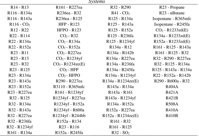
Table 1.3 Mixtures of refrigerants with available data (Last updated 01/10/2016).

Systems

R14 - R13 R161 - R227ea R32 - R290 R23 - Propane

R116 - R134a R236ea - R32 R41 - CO2 R23 - nButane

R116 - R143a R236ea - R125 R125 - R134a Isopentane - R365mfc R116 - CO2 HFP - R123 R125 - R143a Isopentane - R245fa

R12 - R22 HFPO - R123 R125 - R152a CO2 - R1233zd(E)

R22 - R114 CO2 - R32 R125 - R236fa R134a - R1233zd(E)

R22 - R134a CO2 - R134a R125 - R1234yf R152a - R1233zd(E)

R22 - R152a CO2 - R152a R134a - R12 R161 - R125 - R143a

R23 - R11 CO2 - R227ea R134a - R142b R161 - R125 - R32

R23 - R13 CO2 - R1234yf R134a - R227ea R32 - R290 - R227ea

R23 - R32 CO2 - R1234ze(E) R134a - R236fa R32 - R125 - R134a

R23 - R125 CO2 - HFP R134a - R245fa R125 - R143a - R134a

R23 - R134a CO2 - HFPO R134a - R1234yf R22 - R152a - R142b

R23 - R143a R290 - R227ea R134a - R1234ze(E) R290 - R600a - R32

R23 - R152a R3110 - R365mfc R143a - R134a R404A

R23 - R227ea R161 - R1234yf R143a - R161 R421A

R32 - R125 R1234yf - R227ea R143a - R1234yf R421B

R32 - R134a R1234yf - R152a R134a - R152a R508A

R32 - R143a R1234yf - R600a R152a - R227ea R410A

R32 - R227ea R1234yf - R244bb R152a - R1234ze(E) R410B R32 - R236fa R152a - R134 R161 - R32

R32 - R1234yf R23 - R116 R161 - R125 R161 - R134a R152a - R245fa R32 - SO2

In this work, we focus mainly on the new-generation refrigerants, especially the HFO R1234yf, and the two HCFOs R1233xf and R1233zd(E) (pure compounds and mixtures containing at least one of these refrigerants).

From analysing the data gathered, we can summarize the systems of the new-generation refrigerants with data found in the literature along with the references, in Table 1.4 (for the pure compounds), and in Table 1.5 (for the mixtures).