Laboratoire d'Analyse et Modélisation de Systèmes pour l'Aide à la Décision CNRS UMR 7243
CAHIER DU LAMSADE
305
Mars 2011
Weighted completion time minimization on a
single-machine with a fixed non-availability interval:
differential approximability
Weighted Completion Time Minimization on a
Single-Machine with a Fixed Non-Availability
Interval: Differential Approximability
∗Imed Kacem1 and Vangelis Th. Paschos2,3
1LITA, Universit´e Paul Verlaine Metz, France
2LAMSADE, CNRS and Universit´e Paris Dauphine, France
3Institut Universitaire de France
March 14, 2011
Abstract
This paper is the first successful attempt on differential approx-imability study for a scheduling problem. Such a study considers the weighted completion time minimization on a single machine with a fixed non-availability interval. The analysis shows that the Weighted Shortest Processing Time (WSPT) rule cannot yield a differential ap-proximation for the studied problem in the general case. Nevertheless, a slight modification of this rule provides an approximation with a differential ratio of 3−√5
2 ≈ 0.38.
1
Introduction
In this paper, we study the differential approximability of a well-known scheduling problem. Our work is motivated by the fact that the differential approximability concept has not yet been investigated for scheduling prob-lems. Contrary to the standard approximability based on the comparison in the worst case of a heuristic solution to the optimal one, the differential ap-proximability principle consists in comparing the heuristic solution to both the optimal and the worst solutions. More precisely, we say that heuris-tic A is an α-differential approximation for problem Π if for every instance I of Π the following relation holds f (A(I)) ≤ αf (opt(I)) + (1 − α)f (wst(I)), where f is the objective function to be minimized in problem Π and the ∗Research partially supported by the French Agency for Research under the DEFIS program TODO, ANR-09-EMER-010
values opt(I), A(I) and wst(I) denote respectively the values of an opti-mal solution, of an approximate solution and of a worst solution. This last solution is defined as the optimal solution of a problem having the same in-stances and set of constraints with the initial problem but the opposite goal (i.e., max, if the initial problem is a minimization one and min if the initial problem is a maximization problem. Let us also note that worst solutions are not always easy to compute. For instance, for the minimization version of travelling salesman problem, the worst solution is a Hamiltonian cycle of maximum total distance, i.e., the optimum solution of maximum travelling salesman problem. The computation of such a solution is not trivial since the latter problem is as hard as the former one. On the contrary, examples of problems for which a worst solution is easily computed are maximum independent set where the worst solution is the empty set, minimum vertex cover, where this solution is the whole vertex-set of the input graph, or, even, minimum graph-coloring, where the worst solution consists of taking a color per vertex of the input graph. The value α is called the differential ratio and it belongs to (0, 1). For more details on these approaches, the reader is invited to consult Ausiello and Paschos [2] and Demange and Paschos [4].
In the studied problem we have a set of independent jobs to be performed on a single machine under the constraint of a fixed non-availability interval. The objective is to minimize the total weighted completion time under the non-resumable scenario. This problem has been proved to be NP-Hard by Adiri et al. [1] and Lee [13] and it has been studied in the literature under various criteria. Several standard approximations have been proposed. A sample of them include the worst-case analysis of heuristic methods (see for example Adiri et al. [1]; Lee and Liman [15]; Sadfi et al. [16]; He et al. [5]; Wang et al. [19] and Breit [3]; Kacem and Chu [7]; Kacem [9]; Kellerer and Strusevich [12]). Efficient standard approximation schemes were also published in Kellerer and Strusevich [11]; Kacem and Mahjoub [10] and He et al. [5]. Other exact methods to solve this problem have been proposed in Kacem et al. [8]-[6]. For more detail on scheduling problems under non-availability constraints, we refer to the state-of-the-art papers by Lee [14] and Schmidt [17].
The review of the related literature shows that no differential approx-imation has been proposed to this problem according to the best of our knowledge. In a more general way, we did not find any work dedicated to the differential approximation to scheduling problems. For these reasons, this paper is a first successful attempt to develop a polynomial 3−2√5-differential approximation algorithm for the studied problem.
The paper is organized as follows. In Section 2, we present a description of the studied problem. Section 3 provides the differential analysis of the Weighted Shortest Processing Time heuristic (W SP T ). In Section 4, we show that the modification of the above heuristic yields a differential ratio
of 3−2√5. Finally, Section 5 concludes the paper.
2
Problem Formulation
We have to schedule a set of n jobs J = {1, 2, . . . , n} on a single machine. Every job i has a processing time pi and a weight wi. The machine is
un-available between t1 and t2 and it can process at most one job at a time. The
fixed non-availability interval length is denoted by ∆t where ∆t = t2− t1.
Let Ci(σ) denote the completion time of job i in a feasible schedule σ.
The aim is to find a schedule σ∗ that minimizes the total weighted
comple-tion time Pn
i=1wiCi(σ∗). With no loss of generality, we consider that all
data are integers and that jobs are indexed according to the W SP T rule (i.e., p1
w1 ≤
p2
w2 ≤ . . . ≤
pn
wn). Due to the dominance of the W SP T order (see Smith [18]), an optimal schedule is composed of two sequences of jobs sched-uled in nondecreasing order of their indexes (one sequence will be performed before t1 and another after t2).
If all the jobs can be inserted before t1, the problem studied (P) has
obviously a trivial optimal solution obtained by the W SP T rule (Smith [18]). We therefore consider only the problems in which all the jobs cannot be scheduled before t1. The worst solution can be naturally defined as the
solution W ST consisting of scheduling all the jobs after t2 in the W SP T
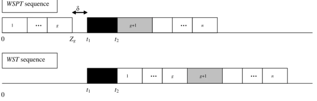
order. Figure 1 illustrates the two sequences W SP T and W ST and the related notations. 1 … g g+1 … n į 0 Zg t1 t2 1 … g g+1 … n t1 t2 WSPT sequence WST sequence 0
Figure 1: Illustration of W SP T and W ST solutions
In the remainder of the paper, we define Zk = k
P
i=1
pi for every k ∈
{1, 2, . . . , n}. Job g is identified by Zg ≤ t1 and Zg+1 > t2. Variable δ
de-notes the idle-time between t1 and the completion time of g in the W SP T
sequence (i.e., δ = t1−Zg). Moreover, ϕ∗(P) denotes the minimum weighted
sum of the completion times for problem P and ϕσ(P) is the weighted sum
3
WSPT Analysis
In this section, we are interested in the differential approximability of the W SP T rule. We recall that the absolute worst-case performance ratio of this rule can be arbitrarily large [13], but not smaller than 3 under some conditions [7]. Our analysis is based upon the comparison of W SP T to W ST and it uses a lower bound introduced in Kacem and Chu [7] (page 1083, Equation (6)).
Lemma 1 [7] The following relation holds:
ϕ∗(P) ≥ g X i=1 wiZi+ wg+1 ∆t pg+1 (Zg+ ∆t) + n X i=g+1 wi(Zi+ ∆t) − wg+1 ∆t pg+1t2
From the definition of W SP T and W ST solutions (Figure 1), the following proposition can directly be established.
Proposition 2 ϕW ST(P) − ϕW SP T(P) = t2 g X i=1 wi+ Zg n X i=g+1 wi Proposition 3 ϕW ST(P) − ϕ∗(P) ≤ t2 g X i=1 wi+ t1 n X i=g+1 wi+ wg+1 ∆t pg+1 δ Proof. From Figure 1, we can establish that:
ϕW ST(P) = n
X
i=1
wi(t2+ Zi) (1)
By combining Lemma (1) and Equation (1), we obtain: ϕW ST(P) − ϕ∗(P) ≤ n X i=1 wi(t2+ Zi) − g X i=1 wiZi− wg+1 ∆t pg+1(Zg+ ∆t) − n X i=g+1 wi(Zi+ ∆t) + wg+1 ∆t pg+1 t2 = t2 g X i=1 wi+ t1 n X i=g+1 wi+ wg+1 ∆t pg+1 (t2− (Zg+ ∆t)) = t2 g X i=1 wi+ t1 n X i=g+1 wi+ wg+1 ∆t pg+1 δ as claimed.
The following well-known lemma will be used in what follows (see also Kacem [9]).
Lemma 4 Let ai and bibe positive numbers (i = 1, 2, . . . , k) such that bi>0
for every i and a1
b1 ≥
a2
b2 ≥ . . . ≥
ak
bk. The following relation holds:
k−1 X i=1 ai k−1 X i=1 bi ≥ abk k (2)
Theorem 5 Let ρ be a positive number such that ρ ∈ (0, 1). If δ ≤ ρt1,
then W SP T is a (1 − ρ)-differential approximation for P, i.e.,
ϕW SP T(P) ≤ (1 − ρ) ϕ∗(P) + ρϕW ST(P) (3)
Proof. Let X and Y be defined as follows:
X = t2 g X i=1 wi+ Zg n X i=g+1 wi Y = t2 g X i=1 wi+ t1 n X i=g+1 wi+ wg+1 ∆t pg+1 δ Hence, Y X = t2 g X i=1 wi+ t1 n X i=g+1 wi+ wg+1p∆tg+1δ t2 g X i=1 wi+ Zg n X i=g+1 wi = 1 + δ n X i=g+1 wi+ wg+1p∆tg+1δ t2 g X i=1 wi+ Zg n X i=g+1 wi ≤ 1 + ρt1 n X i=g+1 wi+ wg+1p∆tg+1δ (1 − ρ) t1 n X i=g+1 wi+ t2 g X i=1 wi = 1 + ρt1 n X i=g+1 wi+ wg+1p∆tg+1δ (1 − ρ) t1 n X i=g+1 wi+ t2 g X i=1 pi ! g X i=1 wi g X i=1 pi
By Lemma 4, it can be established that wg+1 pg+1 ≤ wg pg ≤ g X i=1 wi g X i=1 pi
Moreover, we know that ∆t ≤ t2 and g
P
i=1
pi= Zg. Hence, we deduce that:
Y X ≤ 1 + ρt1 n X i=g+1 wi+ t2wpg+1g+1δ (1 − ρ) t1 n X i=g+1 wi+ t2wpg+1g+1Zg ≤ 1 + ρt1 n X i=g+1 wi+ t2wpg+1g+1ρt1 (1 − ρ) t1 n X i=g+1 wi+ t2wpg+1g+1(1 − ρ) t1 ≤ 1 + ρt1 n X i=g+1 wi+ t2wpg+1g+1 (1 − ρ) t1 n X i=g+1 wi+ t2wpg+1g+1 = 1 (1 − ρ)
From the last result:
ϕW ST(P) − ϕW SP T(P) ϕW ST(P) − ϕ∗(P) ≥ X Y ≥ 1 − ρ ⇒ϕW SP T(P) ≤ (1 − ρ) ϕ∗(P) + ρϕW ST(P) as claimed.
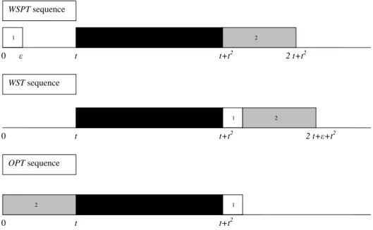
Let us note that, in the general case, W SP T can be arbitrarily bad when δ is large (compared to t1). As an example, let us consider the
tow-job instance with p1 = ε, w1 = ε, p2 = t, w2 = t − ε, t1 = t and t2 = t + t2
(with t >> ε). Figure 2 illustrates the WSPT, WST and OPT solutions. For this instance we have ϕW SP T(P) ≈ t3, ϕW ST(P) ≈ t3 whereas ϕ∗(P) ≈
t2. In other words, the differential approximation ratio in this case tends to 0.
1 0 t t+t2 WSPT sequence WST sequence 2 2 t+t2 1 t t+t2 2 2 t+İ+t2 1 t t+t2 2 OPT sequence 0 0 İ
Figure 2: Worst-case example for W SP T
4
Modifying the WPST Rule to Get a
3−√ 5
2
-Diffe-rential Approximation
Based upon the previous analysis of W SP T rule, it appears that the wrong scheduling of job g + 1 can be the origin of its possible weakness. Hence, we investigate the modification of the W SP T sequence based upon the following algorithm H, which tests the two possibilities of scheduling job g+ 1 before and after the non-availability interval. This algorithm generates two sequences. The first one is the W SP T sequence. In the second one (denoted as W SP T 2), job g + 1 is scheduled before t1 and the other jobs
are scheduled in the W SP T order. The output of this algorithm is the best generated sequence.
HEURISTICH
(i) Construct the sequence W SP T and compute ϕW SP T(P).
(ii) Let y be the yth job in J − {g + 1} according to the WSPT order
(y < g) such that Py
i=1pi + pg+1 ≤ t1 and Py+1i=1 pi + pg+1 > t1.
Construct the sequence:
W SP T2 = h1, 2, . . . , y, g + 1, y + 1, y + 2, . . . , g, g + 2, g + 3, . . . , ni and, if feasible, compute ϕW SP T2(P).
(iii) Output the best among the solutions obtained in steps (i) and (ii) of value ϕH(P) = min {ϕW SP T(P) , ϕW SP T2(P)}.
It can be easily seen that Heuristic H can be implemented in O (n log(n)) time.
To illustrate Heuristic H, let us consider the following four-job instance: p1 = 1; w1 = 2; p2 = 2; w2 = 3; p3 = 3; w3 = 4; p4 = 1; w4 = 1; t1 = 4;
t2 = 7. Given this instance, we have: ϕW SP T(P) = 62; ϕW SP T2(P) = 55
and ϕH(P) = 55. Figure 3 illustrates the obtained schedules. In this case,
we have g = 2 and y = 1.
11
1
7
2
0
4
3
Schedule WSPT10
3
4
1
0
1
7
2
4
9
3
Schedule WSPT210
1
4
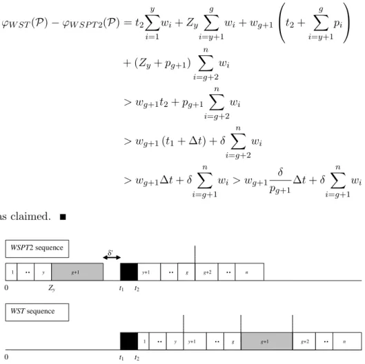
Figure 3: Illustration of H Proposition 6 ϕW ST(P) − ϕW SP T2(P) > wg+1 δ pg+1 ∆t + δ n X i=g+1 wi (4)Proof. From Figure 4, the value ϕW ST(P) − ϕW SP T2(P) can be computed: ϕW ST(P) − ϕW SP T2(P) = t2 y X i=1 wi+ Zy g X i=y+1 wi+ wg+1 t2+ g X i=y+1 pi + (Zy+ pg+1) n X i=g+2 wi > wg+1t2+ pg+1 n X i=g+2 wi > wg+1(t1+ ∆t) + δ n X i=g+2 wi > wg+1∆t + δ n X i=g+1 wi > wg+1 δ pg+1 ∆t + δ n X i=g+1 wi as claimed. 1 … y g+1 … n į' 0 Zy t1 t2 WSPT2 sequence WST sequence y+1 … g g+2 1 … y 0 … g g+2 … n y+1 g+1 t1 t2
Figure 4: Comparison of W SP T 2 with W ST
Theorem 7 Let ρ be a positive number such that ρ ∈ (0, 1). If δ > ρt1,
then H is a (1+ρ)ρ -differential approximation for P, i.e.,
ϕH(P) ≤ ρ (1 + ρ)ϕ ∗(P) + 1 (1 + ρ)ϕW ST(P) (5) Proof. By definition: ϕH(P) = min {ϕW SP T(P), ϕW SP T2(P)} ≤ (1 + ρ)ρ ϕW SP T(P) + 1 (1 + ρ)ϕW SP T2(P)
Hence, ϕW ST(P) − ϕH(P) ≥ ρ (1 + ρ)(ϕW ST(P) − ϕW SP T(P)) + 1 (1 + ρ)(ϕW ST(P) − ϕW SP T2(P)) From Propositions 2 and 6, we can deduce the following inequality:
ϕW ST(P) − ϕH(P) ≥ ρ (1 + ρ) t2 g X i=1 wi+ Zg n X i=g+1 wi + 1 (1 + ρ) wg+1 δ pg+1 ∆t + δ n X i=g+1 wi
By assumption, δ > ρt1. Therefore, we deduce that:
ϕW ST(P) − ϕH(P) > ρ (1 + ρ) t2 g X i=1 wi+ Zg n X i=g+1 wi + 1 (1 + ρ) wg+1 δ pg+1 ∆t + ρt1 n X i=g+1 wi > ρ (1 + ρ) t2 g X i=1 wi ! + ρ (1 + ρ) wg+1 δ pg+1 ∆t + t1 n X i=g+1 wi > ρ (1 + ρ) t2 g X i=1 wi+ t1 n X i=g+1 wi+ wg+1 δ pg+1 ∆t
Finally, from Proposition 3 we obtain: ϕW ST(P) − ϕH(P) ≥
ρ
(1 + ρ)(ϕW ST(P) − ϕ
∗(P)) ,
and then, Equation (5) is proved.
Theorem 8 Heuristic H is a 3−2√5-differential approximation for prob-lem P.
Proof. Let ρ be a positive number such that ρ ∈ (0, 1). By combining Theorems 5 and 7, Heuristic H is a (1+ρ)ρ -differential approximation for P (if δ > ρt1) and a (1 − ρ)-differential approximation for P (if δ ≤ ρt1).
Hence, by taking ρ ∈ (0, 1) such that (1+ρ)ρ = 1 − ρ, we obtain ρ = √
5−1 2 .
Therefore, Heuristic H is a 3−2√5-differential approximation for problem P in the general case:
ϕH(P) ≤ 3 − √ 5 2 ϕ ∗(P) + √ 5 − 1 2 ϕW ST(P) that completes the proof.
5
Conclusion
Motivated by the absence in the literature of differential approximability analysis for scheduling problems, this paper aims to investigate this new direction. The considered study is related to the weighted completion time minimization on a single machine with a fixed non-availability interval. The analysis of the Weighted Shortest Processing Time (W SP T ) rule shows that this rule cannot yield a differential approximation for the studied problem in the general case. Nevertheless, a slight modification of this rule provides a 3−2√5-differential approximation.
Ongoing research will aim at designing more efficient differential approx-imations for scheduling problems (in particular, differential approximation schemes).
References
[1] Adiri, I., Bruno, J., Frostig, E., Rinnooy Kan, A.H.G., 1989. Single ma-chine flow-time scheduling with a single breakdown. Acta Informatica 26, 679-696.
[2] Ausiello, G., Paschos, V.Th., 2006. Reductions, completeness and the hardness of approximability. European Journal of Operational Research 172, 719–739.
[3] Breit, J., 2007. Improved approximation for non-preemptive single ma-chine flow-time scheduling with an availability constraint. European
Journal of Operational Research 183, 516–524.
[4] Demange, M., Paschos, V.Th., 1996. On an approximation measure founded on the links between optimization and polynomial approxima-tion theory. Theoretical Computer Science 158, 117–141.
[5] He, Y., Zhong, W., Gu, H., 2006. Improved algorithms for two single machine scheduling problems. Theoretical Computer Science 363, 257-265.
[6] Kacem, I., Chu, C., 2008. Efficient branch-and-bound algorithm for minimizing the weighted sum of completion times on a single machine with one availability constraint. International Journal of Production
Economics 112:1, 138-150.
[7] Kacem, I., Chu, C., 2008. Worst-case analysis of the WSPT and MWSPT rules for single machine scheduling with one planned setup period. European Journal of Operational Research 187:3, 1080-1089. [8] Kacem, I., Chu, C., Souissi, A., 2008. Single-machine scheduling with an
availability constraint to minimize the weighted sum of the completion times. Computers & Operations Research 35:3, 827-844.
[9] Kacem, I., 2008. Approximation algorithm for the weighted flowtime minimization on a single machine with a fixed non-availability interval.
Computers & Industrial Engineering 54:3, 401-410.
[10] Kacem, I., Mahjoub, A.R., 2009. Fully Polynomial Time Approxima-tion Scheme for the Weighted Flow-time MinimizaApproxima-tion on a Single Ma-chine with a Fixed Non-Availability Interval. Computers & Industrial
Engineering 56:4, 1708-1712.
[11] Kellerer, H., Strusevich, V.A., 2010. Fully Polynomial Approximation Schemes for a Symmetric Quadratic Knapsack Problem and its Schedul-ing Applications. Algorithmica 57:4, 769-795.
[12] Kellerer, H., Kubzin, M.A., Strusevich, V.A., 2009. Two simple con-stant ratio approximation algorithms for minimizing the total weighted completion time on a single machine with a fixed non-availability inter-val. European Journal of Operational Research 199, 111–116.
[13] Lee, C.Y., 1996. Machine scheduling with an availability constraints.
Journal of Global Optimization 9, 363-384.
[14] Lee, C.Y., 2004. Machine scheduling with an availability constraint. In: Leung JYT (Ed), Handbook of scheduling: Algorithms, Models, and
Performance Analysis. USA, FL, Boca Raton, chapter 22.
[15] Lee, C.Y., Liman, S.D., 1992. Single machine flow-time scheduling with scheduled maitenance. Acta Informatica 29, 375-382.
[16] Sadfi, C., Penz, B., Rapine, C., Bla˙zewicz, J., Formanowicz, P., 2005. An improved approximation algorithm for the single machine total com-pletion time scheduling problem with availability constraints. European
Journal of Operational Research 161, 3-10.
[17] Schmidt, G., 2000. Scheduling with limited machine availability.
[18] Smith, W.E., 1956. Various optimizers for single stage production.
Naval Research Logistics Quarterly 3, 59-66.
[19] Wang, G., Sun, H., Chu, C., 2005. Preemptive scheduling with avail-ability constraints to minimize total weighted completion times. Annals